Direction-of-Arrival Estimation for Temporally Correlated Narrowband Signals

Abstract

signal direction-of-arrival estimation using an array of sensors has been the subject of intensive research and development during the last two decades. Efforts have been directed to both, better solutions for the general data model and to develop more realistic models. So far, many authors have assumed the data to be iid samples of a multivariate statistical model. Although this assumption reduces the complexity of the model, it may not be true in certain situations where signals show temporal correlation. Some results are available on the temporally correlated signal model in the literature. The temporally correlated stochastic Cramer-Rao bound (CRB) has been calculated and an instrumental variable-based method called IV-SSF is introduced. Also, it has been shown that temporally correlated CRB is lower bounded by the deterministic CRB. In this paper, we show that temporally correlated CRB is also upper bounded by the stochastic iid CRB. We investigate the effect of temporal correlation of the signals on the best achievable performance. We also show that the IV-SSF method is not efficient and based on an analysis of the CRB, propose a variation in the method which boosts its performance. Simulation results show the improved performance of the proposed method in terms of lower bias and error variance.

I Introduction

Direction-of-Arrival estimation using an array of sensors is widely investigated in the literature in the last decades. Many methods are developed for diverse conditions (see e.g. [1, 2, 3, 4, 5]) and their performances are presented via simulation results or analytical calculations (for papers on theoretical analysis of the performances of the methods see e.g. [6, 7, 8, 9]). Data models play an important role in DOA estimation. They facilitate theoretical derivations of various solutions by their inherent simplistic mathematical and statistical nature. At the same time, overseeing many real-world effects may result in modelling errors and therefore suboptimal methods for the problem at hand. Then, there is a trade-off between simplicity of the models and their usefulness in practice. In the context of array signal processing, there has been considerable research to resolve many aspects of the standard model during the last decades. As a parallel line of research, there also have been efforts to introduce better models which are more application-specific or sometimes more general than the standard model.

In the standard DOA estimation model, snapshots are assumed to be iid or uncorrelated in time. In practice, iid assumption is satisfied with narrowband bandpass filtering of the received signal which gives zero time correlation in certain time delays as ideal sampling points. However, assuming iid snapshots, places a limitation on the applicability of the results in the real world and also forces some practical difficulties. Assuming perfect bandpass filtering of the signal and exact sampling on the zeros of the correlation function, sampling rate should be reduced so that the subsequent samples be uncorrelated. This is a technical difficulty for environments with slowly fluctuating signals when we need large number of samples. Some maximum likelihood methods require the number of observations be at least equal to the number of sensors in order to have a full rank sample covariance matrix $\hat{\boldsymbol{R}}$ [10], at the same time many available DOA estimation methods are efficient only asymptotically in number of snapshots [6]. Then, assuming iid snapshots in theory, results in longer observation times which is not always possible due to moving targets, and may expose us to unpredicted errors due to modelling error. Therefore, it seems useful to accommodate time correlation of at least signals in the model.

Recently, there have been some attempts to tackle with this problem. In [11], authors consider the performance of the spatial covariance-based methods for DOA estimation when signal and noise are not guaranteed to be iid. They conclude that only if noise is still uncorrelated in time, most methods are insensitive to the time correlation of the signals. In [12], an instrumental variable approach (IV-SSF) to the direction-of-arrival estimation problem in the presence of the time correlation of the signals is proposed. The authors improve their previously presented method in [13] to obtain a more reliable approach. The feature of the IV-SSF is that it does not require any knowledge of the noise covariance matrix but its uncorrelatedness in time. In [12], authors also present a statistical performance evaluation for the IV-SSF and calculate some performance bounds for it. In particular, they derive the CRB for the general case of temporally correlated signals and show that it is lower bounded by the well-known deterministic CRB [14]. In another paper in this field [15], authors show the asymptotic equivalence of spatial and temporal IV-SSF methods in a unified framework.

In this paper, we study the properties of the temporally correlated CRB. Although the effect of temporal correlation of the signals on the conventional methods of DOA estimation is investigated in [11], an important remaining question is the role of temporal correlation of the signals in the best achievable performance. Is it helpful or harmful and how much in various conditions? We investigate this issue and show that it is helpful particularly in low SNRs. We also show that the temporally correlated $\textrm{CRB}^{\textrm{cor}}$ is decreasing with the number of samples, as we expect. Then we turn to the IV-SSF to show that it is not an efficient method of DOA estimation in the sense that it cannot achieve the $\textrm{CRB}^{\textrm{cor}}$. Using an asymptotical analysis of the $\textrm{CRB}^{\textrm{cor}}$, we propose an improved version of the IV-SSF which can outperform the existing version. At the end, simulation results confirm the superiority of the new version in terms of lower finite sample bias and estimation error variance.

The remaining of the paper is organized as follows: Section II presents the data model for the temporally correlated signals array processing. Section III is dedicated to the analysis of the CRB properties and a number of new results and comparisons. In section IV the optimality of the IV-SSF in comparison with the $\textrm{CRB}^{\textrm{cor}}$ is investigated and an improvement is proposed. In section V, simulation results are presented to show the better performance of the proposed method. Finally, section VI concludes the paper.

Notation:
$\otimes$ Kronecker product; $\odot$ Hadamard-Schur product; $\|\cdot\|$ matrix Frobenious norm; $(\cdot)^{*}$ conjugate; $(\cdot)^{\textrm{T}}$ transpose; $(\cdot)^{\textrm{H}}$ conjugate transpose; $\textrm{Tr}(\cdot)$ trace; $\textrm{vec}(\cdot)$ vectorizing operator; $\Re$ real part; $\delta_{ij}$ Kronecker delta; $\boldsymbol{a}(\theta_{i})$ array steering vector; $\boldsymbol{A}$ $=[\,\boldsymbol{a}(\theta_{1}),\ldots,\boldsymbol{a}(\theta_{m})]$; steering matrix; $\boldsymbol{D}$ $=[\,\boldsymbol{d}_{1},\ldots,\boldsymbol{d}_{m}]$; $\boldsymbol{d}_{i}=d\boldsymbol{a}(\theta_{i})/d\theta_{i}$; ${\boldsymbol{\Pi}}_{\boldsymbol{A}}^{\bot}$ $\boldsymbol{I}-\boldsymbol{A}(\boldsymbol{A}^{\textrm{H}}\boldsymbol{A})^{-1}\boldsymbol{A}^{\textrm{H}}$; orthogonal projection on to the null space of $\boldsymbol{A}$; $\boldsymbol{A}\geq\boldsymbol{B}$ $\boldsymbol{A}-\boldsymbol{B}$ is positive semi-definite; $\boldsymbol{\mathcal{P}}^{ij}$ $ij$’th block of matrix $\boldsymbol{\mathcal{P}}$; $\boldsymbol{\mathcal{P}}_{ij}$ $ij$’th element of matrix $\boldsymbol{\mathcal{P}}$; $\textrm{BTr}_{m}(\boldsymbol{\mathcal{P}})$ $=\sum_{i}\boldsymbol{\mathcal{P}}^{ii}_{m\times m}$; block trace; $\textrm{Block}_{ij}[\boldsymbol{\mathcal{P}}^{ij}]$ a block matrix with blocks $\boldsymbol{\mathcal{P}}^{ij}$.

II Data Model

Let an array of $L$ sensors receive $n$ samples of the ambient signal and noise. Signal is composed of plane waves from $m$ distant point sources with directions $\boldsymbol{\theta}=[\theta_{1},...,\theta_{m}]$. Spatial correlation between different sources and temporal correlation of the signals are permitted. Noise is assumed to be temporally white. Then, received data can be modelled as

$$\boldsymbol{x}(t)=\boldsymbol{A}(\boldsymbol{\theta})\boldsymbol{s}(t)+\boldsymbol{\nu}(t)$$ (1)

where $\boldsymbol{s}(t)_{m\times 1}$ is the sources signals and $\boldsymbol{\nu}(t)_{L\times 1}$ is the sensors noise vector. Data samples are gathered in matrix form as $\boldsymbol{X}_{L\times n}=[\boldsymbol{x}(t_{1}),\ldots,\boldsymbol{x}(t_{n})]$, and the same is done for the signal sequences $\boldsymbol{S}_{m\times n}=[\boldsymbol{s}(t_{1}),\ldots,\boldsymbol{s}(t_{n})]$ and noise $\boldsymbol{V}_{L\times n}=[\boldsymbol{\nu}(t_{1}),\ldots,\boldsymbol{\nu}(t_{n})]$. Using this notation, the model in (1) can be written as

$$\boldsymbol{X}=\boldsymbol{A}(\boldsymbol{\theta})\boldsymbol{S}+\boldsymbol{V}.$$ (2)

Now, we consider the statistical properties of the model. Regarding the statistics of the signal, three models can be assumed: deterministic, iid, and temporally correlated signal models.

II-1 Deterministic Signal Model

Deterministic signal model assumes a constant signal sequence in every realizations of the process. Then the statistical model of received data will be Gaussian with mean of the signal part and covariance matrix due only to noise

$$\boldsymbol{x}^{det}(t)\sim\mathcal{N}\big{(}\boldsymbol{A}(\boldsymbol{\theta})\boldsymbol{s}(t)\,,\boldsymbol{C}\,\big{)}$$ (3)

$$\boldsymbol{C}=\textrm{E}\big{[}\boldsymbol{\nu}(t)\boldsymbol{\nu}^{\textrm{H}}(t)\big{]}.$$ (4)

II-2 iid Signal Model

In the iid signal model, signal is a random process with the same distribution in every snapshots and no correlation exists between snapshots. Then, data model for the iid case is

$$\boldsymbol{x}^{iid}(t)\sim\mathcal{N}(\boldsymbol{0},\boldsymbol{R})$$ (5)

where

$$\boldsymbol{R}=\boldsymbol{APA}^{\textrm{H}}+\boldsymbol{C}$$ (6)

and

$$\boldsymbol{P}=\textrm{E}\big{[}\boldsymbol{s}(t)\boldsymbol{s}^{\textrm{H}}(t)\big{]}.$$ (7)

II-3 Correlated Signal Model

In the correlated signal model, noise samples are still assumed to be spatially correlated, distributed as a zero-mean Gaussian random vector $\boldsymbol{\nu}(t)\sim\mathcal{N}(\boldsymbol{0},\boldsymbol{C})$, and temporally uncorrelated with $\textrm{E}[\boldsymbol{\nu}(t_{i})\boldsymbol{\nu}^{\textrm{H}}(t_{j})]=\boldsymbol{0}\,,\,i\neq j$. Then, a space-time distribution for noise can be defined as

$$\textrm{vec}(\boldsymbol{V})\sim\mathcal{N}(\boldsymbol{0},\boldsymbol{\mathcal{C}})$$ (8)

$$\boldsymbol{\mathcal{C}}=\boldsymbol{I}_{n}\otimes\boldsymbol{C}.$$ (9)

Similarly, a space-time covariance can be defined for signals. Let $\boldsymbol{\mathcal{P}}^{ij}\triangleq\textrm{E}[\boldsymbol{s}(t_{i})\boldsymbol{s}^{\textrm{H}}(t_{j})]$, then

$$\textrm{vec}(\boldsymbol{S}^{cor})\sim\mathcal{N}(\boldsymbol{0},\boldsymbol{\mathcal{P}})$$ (10)

where $\boldsymbol{\mathcal{P}}_{nm\times nm}=\textrm{Block}_{ij}[\boldsymbol{\mathcal{P}}^{ij}_{m\times m}]$. Now, the space-time distribution of the data under correlated signal model can be easily shown to be

$$\textrm{vec}(\boldsymbol{X}^{cor})\sim\mathcal{N}(\boldsymbol{0},\boldsymbol{\mathcal{R}})$$ (11)

where

$$\boldsymbol{\mathcal{R}}=\boldsymbol{\mathcal{APA}}^{\textrm{H}}+\boldsymbol{\mathcal{C}}$$ (12)

and

$$\boldsymbol{\mathcal{A}}=\boldsymbol{I}_{n}\otimes\boldsymbol{A}(\boldsymbol{\theta}).$$ (13)

Note that (12) has a structure similar to the iid case (6). It is also assumed that $m<L$ and that the array manifold has the property that every set of distinct steering vectors $\{\boldsymbol{a}(\theta_{1}),\cdots,\boldsymbol{a}(\theta_{L})\}$ forms a linearly independent set. Also, $\boldsymbol{a}(\theta)$ is assumed to be a smooth function as it is in real applications which means that $\boldsymbol{d}(\theta)$ exists. These assumptions pave the way for the estimation problem at hand to be identifiable.

III Analysis of the CRB

In this section, we present new results and analyzes on the temporally correlated CRB to give more insight on the estimation problem. We are specially interested in the role of temporal correlation of the signals in the direction estimation problem in comparison with the uncorrelated signal case or iid signals.

CRB is a lower bound on the performance of any unbiased estimation method in terms of error variance. Consider a random vector distributed as $\boldsymbol{y}(t)\sim f(\boldsymbol{\psi})$, where $\boldsymbol{\psi}$ is the vector of possibly unknown parameters of the distribution. Given samples of $\boldsymbol{y}(t)$, an unbiased estimator $\hat{\boldsymbol{\psi}}$ satisfies $\textrm{E}[\hat{\boldsymbol{\psi}}]=\boldsymbol{\psi}$ and its error variance is lower bounded by the CRB as

$$\textrm{E}\big{[}(\hat{\boldsymbol{\psi}}-\boldsymbol{\psi})(\hat{\boldsymbol{\psi}}-\boldsymbol{\psi})^{\textrm{H}}\big{]}\geq\textrm{CRB}_{\boldsymbol{\psi},\boldsymbol{\psi}}.$$ (14)

CRB is an inherent property of the statistical model of the data and can be calculated directly from $f(\boldsymbol{\psi})$. The importance of the CRB also comes from the fact that there exist estimators that at least asymptotically attain the CRB such as the maximum likelihood estimator. In the following, CRB for three discussed signal models are repeated for the sake of reference. In the deterministic signal model of (3) and (4) we have [14]

$$\textrm{CRB}_{\boldsymbol{\theta},\boldsymbol{\theta}}^{\textrm{det}}=\frac{1}{2n}\Big{[}\Re\big{(}\boldsymbol{D}^{\textrm{H}}\boldsymbol{C}^{-\frac{1}{2}}{\boldsymbol{\Pi}}_{0}^{\bot}\boldsymbol{C}^{-\frac{1}{2}}\boldsymbol{D}\big{)}\odot\boldsymbol{P}^{\textrm{T}}\Big{]}^{-1}$$ (15)

where

$${\boldsymbol{\Pi}}_{0}^{\bot}={\boldsymbol{\Pi}}_{\boldsymbol{C}^{-\frac{1}{2}}\boldsymbol{A}}^{\bot}.$$ (16)

In the iid model of (5) and (6) the $\textrm{CRB}^{\textrm{iid}}$ is [14, 16]

$$\textrm{CRB}_{\boldsymbol{\theta},\boldsymbol{\theta}}^{\textrm{iid}}=\frac{1}{2n}\Big{[}\Re\big{(}\boldsymbol{D}^{\textrm{H}}\boldsymbol{C}^{-\frac{1}{2}}{\boldsymbol{\Pi}}_{0}^{\bot}\boldsymbol{C}^{-\frac{1}{2}}\boldsymbol{D}\big{)}\quad\quad$$

$$\odot\big{(}\boldsymbol{PA}^{\textrm{H}}\boldsymbol{R}^{-1}\boldsymbol{A\,P}\big{)}^{\textrm{T}}\Big{]}^{-1}$$ (17)

and in the temporally correlated signal model of (11), (12), and (13) the $\textrm{CRB}^{\textrm{cor}}$ is [12, eq. 112]

$$\textrm{CRB}_{\boldsymbol{\theta},\boldsymbol{\theta}}^{\textrm{cor}}=\frac{1}{2}\Big{[}\Re\big{(}\boldsymbol{D}^{\textrm{H}}\boldsymbol{C}^{-\frac{1}{2}}{\boldsymbol{\Pi}}_{0}^{\bot}\boldsymbol{C}^{-\frac{1}{2}}\boldsymbol{D}\big{)}\qquad\quad$$

$$\odot\,\textrm{BTr}_{m}(\boldsymbol{\mathcal{PG}}^{\textrm{H}}\boldsymbol{\,\mathcal{R^{\prime}}}^{-1}\boldsymbol{\!\mathcal{G\,P}})^{\textrm{T}}\Big{]}^{-1}.$$ (18)

where

$$\boldsymbol{\mathcal{G}}=\boldsymbol{\mathcal{C}}^{-\frac{1}{2}}\boldsymbol{\mathcal{A}}$$ (19)

$$\boldsymbol{\mathcal{R^{\prime}}}=\boldsymbol{\mathcal{GPG}}^{\textrm{H}}+\boldsymbol{\mathcal{I}}=\boldsymbol{\mathcal{C}}^{-\frac{1}{2}}\,\boldsymbol{\mathcal{R}}\,\boldsymbol{\mathcal{C}}^{-\frac{1}{2}}.$$ (20)

where $\boldsymbol{\mathcal{I}}=\boldsymbol{I}_{n}\otimes\boldsymbol{I}_{L}$. It is noteworthy that the expression of the $\textrm{CRB}^{\textrm{cor}}$ in [12] is slightly different from (III) in that it contains a factor of $\frac{1}{n}$ in the right-hand-side. This is a direct consequence of the difference in the definition of the CRB between (14) and what is in [12]. As a confirmation for the form of $\textrm{CRB}^{\textrm{cor}}$ in (III), consider the case of iid signals where the space-time matrices turn out to be block-diagonal. then a factor of $\frac{1}{n}$ appears in the right-hand-side to reduce the $\textrm{CRB}^{\textrm{cor}}$ in (III) to the $\textrm{CRB}^{\textrm{iid}}$ in (III).

To proceed further, we first give a simplified form of the $\textrm{CRB}^{\textrm{cor}}$ in (III). Note that

$$\boldsymbol{\mathcal{G}}^{\textrm{H}}\boldsymbol{\,\mathcal{R^{\prime}}}^{-1}\boldsymbol{\!\mathcal{G}}=\boldsymbol{\mathcal{A}}^{\textrm{H}}\boldsymbol{\,\mathcal{R}}^{-1}\boldsymbol{\!\mathcal{A}}$$ (21)

then the $\textrm{CRB}^{\textrm{cor}}$ can be written as

$$\textrm{CRB}_{\boldsymbol{\theta},\boldsymbol{\theta}}^{\textrm{cor}}=\frac{1}{2}\Big{[}\Re\big{(}\boldsymbol{D}^{\textrm{H}}\boldsymbol{C}^{-\frac{1}{2}}{\boldsymbol{\Pi}}_{0}^{\bot}\boldsymbol{C}^{-\frac{1}{2}}\boldsymbol{D}\big{)}\qquad\quad$$

$$\odot\,\textrm{BTr}_{m}(\boldsymbol{\mathcal{PA}}^{\textrm{H}}\boldsymbol{\,\mathcal{R}}^{-1}\boldsymbol{\!\mathcal{A\,P}})^{\textrm{T}}\Big{]}^{-1}.$$ (22)

Now, we are ready to state our first result on the comparison of the CRB in the signal models introduced.

Theorem 1

For the deterministic signal model in (3) and (4), iid signal model in (5) and (6), and the temporally correlated signal model in (11) and (12), $\textrm{CRB}^{\textrm{cor}}$ is upper bounded by $\textrm{CRB}^{\textrm{iid}}$ and lower bounded by $\textrm{CRB}^{\textrm{det}}$

$$\textrm{CRB}^{\textrm{det}}\leq\textrm{CRB}^{\textrm{cor}}\leq\textrm{CRB}^{\textrm{iid}}.$$ (23)

Proof:

The left side inequality is proved in [12], therefore we give a proof for the right side inequality. We make use of a form of the Woodburry identity [17, 18] which states that

$$(\boldsymbol{A}+\boldsymbol{BCD})^{-1}=\qquad\qquad\qquad\qquad\qquad\qquad$$

$$\boldsymbol{A}^{-1}-\boldsymbol{A}^{-1}\boldsymbol{B}(\boldsymbol{I}+\boldsymbol{CDA}^{-1}\boldsymbol{B})^{-1}\boldsymbol{CDA}^{-1}$$ (24)

which is essentially another form of the matrix inversion lemma. Now we expand the space-time matrix in the block trace of (III) substituting from (12) and making use of (III) to have

$$\boldsymbol{\mathcal{PA}}^{\textrm{H}}\boldsymbol{\,\mathcal{R}}^{-1}\boldsymbol{\!\mathcal{A\,P}}=\boldsymbol{\mathcal{PA}}^{\textrm{H}}\big{[}\boldsymbol{\mathcal{C}}^{-1}-\qquad\quad\qquad\qquad$$

$$\boldsymbol{\mathcal{C}}^{-1}\boldsymbol{\mathcal{A}}\,(\boldsymbol{\mathcal{I}}+\boldsymbol{\mathcal{PA}}^{\textrm{H}}\boldsymbol{\mathcal{C}}^{-1}\boldsymbol{\mathcal{A}})^{-1}\,\boldsymbol{\mathcal{PA}}^{\textrm{H}}\boldsymbol{\mathcal{C}}^{-1}\big{]}\boldsymbol{\mathcal{AP}}=$$

$$\boldsymbol{\mathcal{PA}}^{\textrm{H}}\boldsymbol{\mathcal{C}}^{-1}\boldsymbol{\mathcal{AP}}-\boldsymbol{\mathcal{PA}}^{\textrm{H}}\boldsymbol{\mathcal{C}}^{-1}\boldsymbol{\mathcal{A}}(\boldsymbol{\mathcal{I}}+\qquad$$

$$\boldsymbol{\mathcal{PA}}^{\textrm{H}}\boldsymbol{\mathcal{C}}^{-1}\boldsymbol{\mathcal{A}})^{-1}\boldsymbol{\mathcal{PA}}^{\textrm{H}}\boldsymbol{\mathcal{C}}^{-1}\boldsymbol{\mathcal{AP}}.$$ (25)

We factor the common terms of (III) from right side to get

$$\big{[}\boldsymbol{\mathcal{I}}-\boldsymbol{\mathcal{PA}}^{\textrm{H}}\boldsymbol{\mathcal{C}}^{-1}\boldsymbol{\mathcal{A}}\,(\boldsymbol{\mathcal{I}}+\qquad\qquad\qquad$$

$$\boldsymbol{\mathcal{PA}}^{\textrm{H}}\boldsymbol{\mathcal{C}}^{-1}\boldsymbol{\mathcal{A}})^{-1}\big{]}\boldsymbol{\mathcal{PA}}^{\textrm{H}}\boldsymbol{\mathcal{C}}^{-1}\boldsymbol{\mathcal{AP}}.$$ (26)

Add and subtract an $\boldsymbol{\mathcal{I}}$ to the $\boldsymbol{\mathcal{PA}}^{\textrm{H}}\boldsymbol{\mathcal{C}}^{-1}\boldsymbol{\mathcal{A}}$ in the bracket in (III) to get

$$(\boldsymbol{\mathcal{I}}+\boldsymbol{\mathcal{PA}}^{\textrm{H}}\boldsymbol{\mathcal{C}}^{-1}\boldsymbol{\mathcal{A}})^{-1}\boldsymbol{\mathcal{PA}}^{\textrm{H}}\boldsymbol{\mathcal{C}}^{-1}\boldsymbol{\mathcal{AP}}.$$ (27)

Do the same for the term outside the bracket in (27) in the following form

$$(\boldsymbol{\mathcal{I}}+\boldsymbol{\mathcal{PA}}^{\textrm{H}}\boldsymbol{\mathcal{C}}^{-1}\boldsymbol{\mathcal{A}})^{-1}(\boldsymbol{\mathcal{I}}+\boldsymbol{\mathcal{PA}}^{\textrm{H}}\boldsymbol{\mathcal{C}}^{-1}\boldsymbol{\mathcal{A}}-\boldsymbol{\mathcal{I}})\boldsymbol{\mathcal{P}}.$$ (28)

As a useful result, we arrive to the following equality simplifying (28)

$$\boldsymbol{\mathcal{PA}}^{\textrm{H}}\boldsymbol{\,\mathcal{R}}^{-1}\boldsymbol{\!\mathcal{A\,P}}=\boldsymbol{\mathcal{P}}-(\boldsymbol{\mathcal{P}}^{-1}+\boldsymbol{\mathcal{A}}^{\textrm{H}}\boldsymbol{\mathcal{C}}^{-1}\boldsymbol{\mathcal{A}})^{-1}.$$ (29)

Note that the matrix in parenthesis is positive semi-definite, then we will have

$$\boldsymbol{\mathcal{PA}}^{\textrm{H}}\boldsymbol{\,\mathcal{R}}^{-1}\boldsymbol{\!\mathcal{A\,P}}\leq\boldsymbol{\mathcal{P}}$$ (30)

which is another proof for the left side inequality in (23) (see [12]). Now, we proceed to prove the right side inequality in (23). define

$$\boldsymbol{\mathcal{P}}_{d}\triangleq\textrm{Block}_{ij}[\boldsymbol{\mathcal{P}}^{ij}\delta_{ij}]$$ (31)

which is the block-diagonalized version of the signal space-time covariance matrix. Note that block-diagonal space-time covariance matrix for signals $\boldsymbol{\mathcal{P}}_{d}$, represents the temporally uncorrelated signal model (more general than iid signal model), while $\boldsymbol{\mathcal{P}}$ represents the temporally correlated signal model. Now, assume a matrix $\boldsymbol{\mathcal{F}}$ and its block-diagonalized version $\boldsymbol{\mathcal{F}}_{d}$. It is well known that

$$(\boldsymbol{\mathcal{F}}^{-1})^{ii}\geq(\boldsymbol{\mathcal{F}}^{ii})^{-1}=(\boldsymbol{\mathcal{F}}_{d}^{ii})^{-1}=(\boldsymbol{\mathcal{F}}_{d}^{-1})^{ii}.$$ (32)

Using the inequality in (32), besides the fact that $\boldsymbol{\mathcal{A}}^{\textrm{H}}\boldsymbol{\mathcal{C}}^{-1}\boldsymbol{\mathcal{A}}$ is block-diagonal, we will have

$$\boldsymbol{\mathcal{A}}^{\textrm{H}}\boldsymbol{\mathcal{C}}^{-1}\boldsymbol{\mathcal{A}}-\big{(}\boldsymbol{\mathcal{P}}+(\boldsymbol{\mathcal{A}}^{\textrm{H}}\boldsymbol{\mathcal{C}}^{-1}\boldsymbol{\mathcal{A}})^{-1}\big{)}^{-1}\leq\qquad$$

$$\boldsymbol{\mathcal{A}}^{\textrm{H}}\boldsymbol{\mathcal{C}}^{-1}\boldsymbol{\mathcal{A}}-\big{(}\boldsymbol{\mathcal{P}}_{d}+(\boldsymbol{\mathcal{A}}^{\textrm{H}}\boldsymbol{\mathcal{C}}^{-1}\boldsymbol{\mathcal{A}})^{-1}\big{)}^{-1}$$ (33)

Now, we multiply $\boldsymbol{\mathcal{B}}\triangleq(\boldsymbol{\mathcal{A}}^{\textrm{H}}\boldsymbol{\mathcal{C}}^{-1}\boldsymbol{\mathcal{A}})^{-1}$ from right and left of both sides of the inequality to get

$$\boldsymbol{\mathcal{B}}-\boldsymbol{\mathcal{B}}\big{(}\boldsymbol{\mathcal{P}}+\boldsymbol{\mathcal{B}}\big{)}^{-1}\boldsymbol{\mathcal{B}}\leq\boldsymbol{\mathcal{B}}-\boldsymbol{\mathcal{B}}\big{(}\boldsymbol{\mathcal{P}}_{d}+\boldsymbol{\mathcal{B}}\big{)}^{-1}\boldsymbol{\mathcal{B}}.$$ (34)

The above expressions can be simplified using matrix inversion lemma to give

$$\big{(}\boldsymbol{\mathcal{P}}^{-1}+\boldsymbol{\mathcal{A}}^{\textrm{H}}\boldsymbol{\mathcal{C}}^{-1}\boldsymbol{\mathcal{A}}\big{)}^{-1}\leq\big{(}\boldsymbol{\mathcal{P}}_{d}^{-1}+\boldsymbol{\mathcal{A}}^{\textrm{H}}\boldsymbol{\mathcal{C}}^{-1}\boldsymbol{\mathcal{A}}\big{)}^{-1}.$$ (35)

Applying the block trace operator and adding a common term results in

$$\textrm{BTr}_{m}\big{[}\boldsymbol{\mathcal{P}}-\big{(}\boldsymbol{\mathcal{P}}^{-1}+\boldsymbol{\mathcal{A}}^{\textrm{H}}\boldsymbol{\mathcal{C}}^{-1}\boldsymbol{\mathcal{A}}\big{)}^{-1}\big{]}\geq\qquad\qquad$$

$$\textrm{BTr}_{m}\big{[}\boldsymbol{\mathcal{P}}_{d}-\big{(}\boldsymbol{\mathcal{P}}_{d}^{-1}+\boldsymbol{\mathcal{A}}^{\textrm{H}}\boldsymbol{\mathcal{C}}^{-1}\boldsymbol{\mathcal{A}}\big{)}^{-1}\big{]}.$$ (36)

According to (29), the inequality in (III) implies that

$$\textrm{BTr}_{m}\big{[}\boldsymbol{\mathcal{PA}}^{\textrm{H}}\boldsymbol{\,\mathcal{R}}^{-1}\boldsymbol{\!\mathcal{A\,P}}\big{]}\geq\qquad\qquad$$

$$\textrm{BTr}_{m}\big{[}\boldsymbol{\mathcal{P}}_{d}\boldsymbol{\mathcal{A}}^{\textrm{H}}\boldsymbol{\,\mathcal{R}}_{d}^{-1}\boldsymbol{\!\mathcal{A\,P}}_{d}\big{]}.$$ (37)

which in fact completes the proof of (23) showing that

$$\textrm{CRB}^{\textrm{cor}}(\boldsymbol{\mathcal{P}})\leq\textrm{CRB}^{\textrm{cor}}(\boldsymbol{\mathcal{P}}_{d}).$$ (38)

∎

The upper bound and lower bound on the $\textrm{CRB}^{\textrm{cor}}$ presented in (23) is very insightful to the estimation problem at hand. It implies that the existence of a temporal correlation in the signals improve the best attainable performance of estimation. The comparison made in theorem 1 is conditioned on the specific spatial covariance matrix of the sources in each sample i.e. with the same diagonal blocks of the space-time signal covariance matrix. It shows that adding a nondiagonal covariance block improves the performance since it simplifies the extraction of the signal part from received data. Most spatial covariance-based DOA estimation methods rely on the different spatial characteristics of the signal and noise (signals are point sources of radiation while noise is uniformly distributed in the space or at least is spread via large areas). This is not the case in the temporally correlated signal model where there is a particular difference between signal and noise in that one is temporally correlated and the other is temporally uncorrelated. This increased distance of the signal model and noise model improves the CRB and the performance of the methods using it. As a result, we can see that the $\textrm{CRB}^{\textrm{cor}}$ is lower than the $\textrm{CRB}^{\textrm{iid}}$ which implies better performance when noise and signal have different temporal characteristics. Another explanation for the inequalities presented in (23) comes from the degree of predictability of the signal. It is obvious that in the deterministic signal model we have a statistically constant signal which is fully predictable. Therefore, the performance is best in the deterministic signal model. In the correlated signal model, signals are stochastic in nature and vary in each realization, which makes the signals less predictable. Though, the existence of the temporal correlation of the signals offers a limited possibility for coarse signal prediction and extraction from noise which places the $\textrm{CRB}^{\textrm{cor}}$ lower than the completely uncorrelated case of $\textrm{CRB}^{\textrm{iid}}$.

Although we have confined the $\textrm{CRB}^{\textrm{cor}}$ between $\textrm{CRB}^{\textrm{det}}$ and $\textrm{CRB}^{\textrm{iid}}$ in theorem 1, we are interested to more exactly specify the behavior of the $\textrm{CRB}^{\textrm{cor}}$ in different situations. This helps us to get more insight to the role of temporal correlation of the signals in DOA estimation. Therefore we consider approximations of the $\textrm{CRB}^{\textrm{cor}}$ in different situations in temrs of signal to noise ratio (SNR) in the following theorem.

Theorem 2

In the high SNR condition, temporal correlation of the signals makes no improvement on the uncorrelated signal model while in the low SNR condition, the contribution of zero-lag and nonzero-lag covariances are the same, i.e. nonzero-lag covariances improve the CRB.

$$\textrm{SNR}\gg 1:\quad\textrm{CRB}^{\textrm{cor}}\simeq\textrm{CRB}^{\textrm{iid}}$$ (39)

$$\textrm{SNR}\ll 1:\quad\textrm{CRB}^{\textrm{cor}}<\textrm{CRB}^{\textrm{iid}}$$ (40)

Proof:

Consider the high SNR condition. We make use of the following easily checked approximation for any appropriately sized matrices $\boldsymbol{B}$ and $\boldsymbol{\Delta}$ if $\|\boldsymbol{\Delta}\|\leq\|\boldsymbol{B}\|$

$$(\boldsymbol{B}+\boldsymbol{\Delta})^{-1}\simeq\boldsymbol{B}^{-1}-\qquad\qquad\qquad\qquad\qquad$$

$$\boldsymbol{B}^{-1}\boldsymbol{\Delta}\boldsymbol{B}^{-1}+\boldsymbol{B}^{-1}\boldsymbol{\Delta}\boldsymbol{B}^{-1}\boldsymbol{\Delta}\boldsymbol{B}^{-1}-\cdots$$ (41)

Now we can expand the block trace in $\textrm{CRB}^{\textrm{cor}}$ as follows

$$\textrm{BTr}_{m}\big{[}\boldsymbol{\mathcal{PA}}^{\textrm{H}}\boldsymbol{\,\mathcal{R}}^{-1}\boldsymbol{\!\mathcal{A\,P}}\big{]}=\qquad\qquad\qquad\qquad$$

$$\textrm{BTr}_{m}\big{[}\boldsymbol{\mathcal{P}}\boldsymbol{\mathcal{A}}^{\textrm{H}}(\boldsymbol{\mathcal{C}}+\boldsymbol{\mathcal{APA}}^{\textrm{H}})^{-1}\boldsymbol{\!\mathcal{A\,P}}\big{]}.$$ (42)

We use matrix inversion lemma for the inverse in the block trace of (III) to get

$$\textrm{BTr}_{m}\big{[}\boldsymbol{\mathcal{P}}\boldsymbol{\mathcal{A}}^{\textrm{H}}\big{(}\boldsymbol{\mathcal{C}}^{-1}-\boldsymbol{\mathcal{C}}^{-1}\boldsymbol{\mathcal{A}}(\boldsymbol{\mathcal{P}}^{-1}+\qquad$$

$$\boldsymbol{\mathcal{A}}^{\textrm{H}}\boldsymbol{\mathcal{C}}^{-1}\boldsymbol{\mathcal{A}})^{-1}\boldsymbol{\mathcal{A}}^{\textrm{H}}\boldsymbol{\mathcal{C}}^{-1}\big{)}\boldsymbol{\mathcal{A\,P}}\big{]}.$$ (43)

Now we use the approximation in (III) up to the third term. Note that the high SNR assumption guarantees that $\|\boldsymbol{\mathcal{P}}^{-1}\|\leq\|\boldsymbol{\mathcal{A}}^{\textrm{H}}\boldsymbol{\mathcal{C}}^{-1}\boldsymbol{\mathcal{A}}\|$. After some calculations we get

$$\textrm{BTr}_{m}\big{[}\boldsymbol{\mathcal{PA}}^{\textrm{H}}\boldsymbol{\,\mathcal{R}}^{-1}\boldsymbol{\!\mathcal{A\,P}}\big{]}\simeq\qquad\qquad\qquad\qquad$$

$$\textrm{BTr}_{m}\big{[}\boldsymbol{\mathcal{P}}-(\boldsymbol{\mathcal{A}}^{\textrm{H}}\boldsymbol{\mathcal{C}}^{-1}\boldsymbol{\mathcal{A}})^{-1}\big{]}$$ (44)

in the high SNR region and to the second order of approximation. The approximation in (III) asserts that in high SNR condition, only block trace of the signal space-time covariance matrix contribute to the Cramer-Rao bound, hence we can conclude that in this case, the temporal correlation of the signals (represented by nondiagonal blocks of $\boldsymbol{\mathcal{P}}$), do not improve the best achievable performance of the DOA estimation and (39) follows.

In the very low SNR region, we use the approximation $\boldsymbol{\mathcal{R}}\simeq\boldsymbol{\mathcal{C}}$. Then expanding the block trace in the CRB gives

$$\textrm{BTr}_{m}\big{[}\boldsymbol{\mathcal{PA}}^{\textrm{H}}\boldsymbol{\,\mathcal{R}}^{-1}\boldsymbol{\!\mathcal{A\,P}}\big{]}\simeq\qquad$$

$$\sum_{i,r}\,(\boldsymbol{A\mathcal{P}}^{ri})^{\textrm{H}}\boldsymbol{C}^{-1}(\boldsymbol{A\mathcal{P}}^{ri}).$$ (45)

We can see from (III) that every blocks of $\boldsymbol{\mathcal{P}}$ contribute the same to the $\textrm{CRB}^{\textrm{cor}}$ in the situation of very low SNR. Since each term in the summation of (III) is positive semi-definite, then each nondiagonal block of $\boldsymbol{\mathcal{P}}$ improves the $\textrm{CRB}^{\textrm{cor}}$ making the distance from $\textrm{CRB}^{\textrm{iid}}$ larger which implies (40). It is noteworthy that improvement of the CRB does not mean the performance improvement of the conventional DOA estimation methods, rather it clarifies the existence of methods that can achieve better performances through making use of the temporal characteristics of the signals and noise. ∎

Now, after we considered the role of the temporal correlation of the signals in the best achievable performance of DOA estimation, we turn to an assumed characteristic of the CRB. The CRB usually decreases with increased amount of data. This is obvious in the iid signal models where the CRB for $n$ data samples is $\frac{1}{n}$ of the CRB for one sample. Though, this is not very clear for the temporally correlated signal model where the dependence of the $\textrm{CRB}^{\textrm{cor}}$ on $n$ is embedded in the size of the space-time matrices.

Theorem 3

$\textrm{CRB}^{\textrm{cor}}$ is decreasing with increasing $n$.

$$\textrm{CRB}^{\textrm{cor}}(n+1)<\textrm{CRB}^{\textrm{cor}}(n).$$ (46)

Proof:

Applying matrix inversion lemma, we can show that

$$\boldsymbol{\mathcal{A}}^{\textrm{H}}\boldsymbol{\mathcal{R}}^{-1}\boldsymbol{\mathcal{A}}=\big{(}\boldsymbol{\mathcal{P}}+(\boldsymbol{\mathcal{A}}^{\textrm{H}}\boldsymbol{\mathcal{C}}^{-1}\boldsymbol{\mathcal{A}})^{-1}\big{)}^{-1}.$$ (47)

Assuming $\boldsymbol{\mathcal{P}}_{n+1}$ as the block-diagonally augmented version of $\boldsymbol{\mathcal{P}}_{n}$ and using (47), we will have

$$\textrm{CRB}^{\textrm{cor}}\Big{(}\left[\!\!\begin{array}[]{l}\boldsymbol{\mathcal{P}}_{n}\\ \qquad\boldsymbol{P}_{n+1}\end{array}\!\!\right]\Big{)}\leq\textrm{CRB}^{\textrm{cor}}(\boldsymbol{\mathcal{P}}_{n}).$$ (48)

since

$$\textrm{BTr}_{m}[\boldsymbol{\mathcal{P}}_{n+1}\boldsymbol{\mathcal{A}}^{\textrm{H}}_{n+1}\boldsymbol{\,\mathcal{R}}^{-1}_{n+1}\boldsymbol{\mathcal{A}}_{n+1}\boldsymbol{\mathcal{P}}_{n+1}\big{]}=\qquad\qquad$$

$$\textrm{BTr}_{m}\big{[}\boldsymbol{\mathcal{P}}_{n}(\boldsymbol{\mathcal{P}}_{n}+(\boldsymbol{\mathcal{A}}_{n}^{\textrm{H}}\boldsymbol{\mathcal{C}}^{-1}_{n}\boldsymbol{\mathcal{A}}_{n})^{-1})^{-1}\boldsymbol{\mathcal{P}}_{n}\big{]}+\qquad$$

$$\boldsymbol{P}_{n+1}\big{(}\boldsymbol{P}_{n+1}+(\boldsymbol{A}^{\textrm{H}}\boldsymbol{C}^{-1}\boldsymbol{A})^{-1}\big{)}^{-1}\boldsymbol{P}_{n+1}$$ (49)

and the second term is positive semi-definite. Following the same steps as in (III) to (38), we can also show the following inequality which completes the proof.

$$\textrm{CRB}^{\textrm{cor}}\Big{(}\left[\!\!\begin{array}[]{lc}\boldsymbol{\mathcal{P}}_{n}&\boldsymbol{Q}^{\textrm{H}}\\ \boldsymbol{Q}&\boldsymbol{P}_{n+1}\end{array}\!\!\right]\Big{)}\leq\textrm{CRB}^{\textrm{cor}}\Big{(}\left[\!\!\begin{array}[]{l}\boldsymbol{\mathcal{P}}_{n}\\ \qquad\boldsymbol{P}_{n+1}\end{array}\!\!\right]\Big{)}$$ (54)

Note that, (54) is a generalization of the R.H.S. inequality in (23). ∎

In this section, we investigated the general properties of the direction-of-arrival estimation problem in the presence of the temporally correlated signals. We performed this via Cramer-Rao bound analysis and characterization. In the next section we turn to the practical methods to accomplish DOA estimation under temporally correlated signal model.

IV Suboptimality of the IV-SSF Method

We have considered the best achievable performance in the temporally correlated signal model. In particular, we found that it is possible to improve the performance of the conventional spatial covariance-based methods by devising new methods that can exploit the temporal correlation of the signals. However, the $\textrm{CRB}^{\textrm{cor}}$ has been calculated under the assumption of known noise spatial covariance matrix. When this is not true, we do not expect any method to reach the $\textrm{CRB}^{\textrm{cor}}$ in performance. In the situation of unknown noise spatial covariance matrix, the instrumental variable subspace fitting (IV-SSF) method for direction-of-arrival estimation has been proposed in [12]. The method is based on the instrumental variable approach. It makes an instrumental variables vector $\boldsymbol{\phi}(t)$ for each data sample $\boldsymbol{x}(t)$ in such a way that the cross-covariance of $\boldsymbol{\phi}(t)$ and $\boldsymbol{x}(t)$ does not contain the unknown noise covariance matrix. Then, a sample cross-covariance can be used to extract the signal subspace and parameters of interest. Note that the signal temporal correlation leave a room for the multiplication of noncontemporary data to contain information about the directions of arrival. The instrumental variables vector for each data sample $\boldsymbol{x}(t)$ is formed as

$$\boldsymbol{\phi}(t)\triangleq\left[\!\!\begin{array}[]{c}\boldsymbol{x}(t-1)\\ \vdots\\ \boldsymbol{x}(t-M)\end{array}\!\!\right]$$ (55)

where $M$ is a user defined integer determining the degree of complexity and hence the performance of the method. In general, larger $M$ should result in better estimates, although simulation results show increased bias and decreased error variance when $M$ becomes larger. Let the cross-covariance of the signals at time lag $k$ be defined as

$$\boldsymbol{P}_{k}\triangleq\textrm{E}[\boldsymbol{s}(t-k)\boldsymbol{s}^{\textrm{H}}(t)]$$ (56)

and define for convenience

$$\boldsymbol{\mathcal{J}}=\left[\!\!\begin{array}[]{c}\boldsymbol{P}_{1}\\ \vdots\\ \boldsymbol{P}_{M}\end{array}\!\!\!\right]$$ (57)

then the cross-covariance of the received data and the corresponding instrumental variable will be

$$\boldsymbol{\Sigma}\triangleq\textrm{E}[\boldsymbol{\phi}(t)\boldsymbol{x}^{\textrm{H}}(t)]=(\boldsymbol{I}_{M}\otimes\boldsymbol{A})\,\boldsymbol{\mathcal{J}}\boldsymbol{A}^{\textrm{H}}$$ (58)

which is independent of the unknown noise spatial covariance matrix $\boldsymbol{C}$. Also define the instrumental variable covariance matrix as

$$\boldsymbol{\Phi}\triangleq\textrm{E}[\boldsymbol{\phi}(t)\boldsymbol{\phi}^{\textrm{H}}(t)].$$ (59)

The estimates of the DOAs in IV-SSF method are obtained in the following steps: choose $M>1$ and compute the sample estimates

$$\hat{\boldsymbol{\Sigma}}=\frac{1}{n-M}\!\!\!\sum_{\;\;t=M+1}^{n}\!\!\!\boldsymbol{\phi}(t)\boldsymbol{x}^{\textrm{H}}(t)$$ (60)

$$\hat{\boldsymbol{\Phi}}=\frac{1}{n-M}\!\!\!\sum_{\;\;t=M+1}^{n}\!\!\!\boldsymbol{\phi}(t)\boldsymbol{\phi}^{\textrm{H}}(t).$$ (61)

Next, extract $\hat{\boldsymbol{R}}_{0}$ from $\hat{\boldsymbol{\Phi}}$, as one of the $m\times m$ diagonal blocks. The estimates of the parameters are the minimizer of the following criterion function:

$$\hat{\boldsymbol{\theta}}=\arg\;\min_{\boldsymbol{\theta}}\,\textrm{Tr}\,\Big{(}\hat{\boldsymbol{\Pi}}_{0}^{\bot}\hat{\boldsymbol{R}}_{0}^{-\frac{1}{2}}\hat{\boldsymbol{V}}_{s}\hat{\boldsymbol{\Phi}}_{s}^{2}\hat{\boldsymbol{V}}_{s}^{\textrm{H}}\hat{\boldsymbol{R}}_{0}^{-\frac{1}{2}}\Big{)}$$ (62)

where

$$\hat{\boldsymbol{\Pi}}_{0}^{\bot}=\boldsymbol{I}-\hat{\boldsymbol{R}}_{0}^{-\frac{1}{2}}\boldsymbol{A}\big{(}\boldsymbol{A}^{\textrm{H}}\hat{\boldsymbol{R}}_{0}^{-1}\boldsymbol{A}\big{)}^{-1}\boldsymbol{A}^{\textrm{H}}\hat{\boldsymbol{R}}_{0}^{-\frac{1}{2}}$$ (63)

and $\hat{\boldsymbol{V}}_{s}$ contains the dominant right singular vectors of the matrix $\hat{\boldsymbol{\Phi}}^{-\frac{1}{2}}\hat{\boldsymbol{\Sigma}}$, while the associated singular values are gathered in matrix $\hat{\boldsymbol{\Phi}}_{s}$.

Using the IV-SSF method, the asymptotic error covariance matrix has been shown to be [12]

$$\textrm{Cov}^{\textrm{IV-SSF}}=\frac{1}{2n}\Big{[}\Re\big{(}\boldsymbol{D}^{\textrm{H}}\boldsymbol{C}^{-\frac{1}{2}}{\boldsymbol{\Pi}}_{0}^{\bot}\boldsymbol{C}^{-\frac{1}{2}}\boldsymbol{D}\big{)}\odot\qquad\quad$$

$$\big{(}\boldsymbol{\mathcal{J}}^{\,\textrm{H}}\boldsymbol{\mathcal{A}}_{M}^{\textrm{H}}\,\boldsymbol{\Phi}^{-1}\boldsymbol{\mathcal{A}}_{M}\boldsymbol{\mathcal{J}}\big{)}^{\textrm{T}}\Big{]}^{-1}$$ (64)

in which $\boldsymbol{\mathcal{A}}_{M}=\boldsymbol{I}_{M}\otimes\boldsymbol{A}$. The covariance in (IV) is slightly different from the $\textrm{CRB}^{\textrm{cor}}$ in (III). We aim to show that the IV-SSF method with above error covariance does not attain the $\textrm{CRB}^{\textrm{cor}}$ asymptotically and relying on this analysis, we propose a variation in the method to boost its performance. To this end, we use an asymptotic analysis presented in [12] with some modifications to be able to compare the $\textrm{CRB}^{\textrm{cor}}$ and the covariance in (IV). Define an estimation problem in which we are interested to estimate the signal $\boldsymbol{s}(t)$ using the data $\boldsymbol{z}(t)=\boldsymbol{s}(t)+\boldsymbol{w}(t)$, in which $\boldsymbol{w}(t)$ is a temporally white noise term with spatial covariance matrix $(\boldsymbol{A}^{\textrm{H}}\boldsymbol{C}^{-1}\boldsymbol{A})^{-1}$. Note that $\boldsymbol{w}(t)$ is temporally white since it is constructed from iid noise term $\boldsymbol{\nu}(t)$ by a linear transform in the space domain. Assume that we are to estimate $\boldsymbol{s}(t)$ from $M$ previous samples of $\boldsymbol{z}(t)$

$$\boldsymbol{z}_{M}(t)=\big{[}\,\boldsymbol{z}^{\textrm{T}}(t-1)\quad\cdots\quad\boldsymbol{z}^{\textrm{T}}(t-M)\,\big{]}^{\textrm{T}}.$$ (65)

with the best linear transform which minimizes the error covariance matrix. The estimation error will be

$$\boldsymbol{s}(t)-\boldsymbol{{\mathcal{H}}z}_{M}(t)=\boldsymbol{e}(t)$$ (66)

where $\boldsymbol{\mathcal{H}}$ is the best linear transform in the least squares sense. Making use of the orthogonality principle, we can show that

$$\hat{\boldsymbol{\mathcal{H}}}=\boldsymbol{\mathcal{J}}^{\textrm{H}}\big{(}\boldsymbol{\mathcal{P}}_{M}+(\boldsymbol{\mathcal{A}}_{M}^{\textrm{H}}\boldsymbol{\mathcal{C}}_{M}^{-1}\boldsymbol{\mathcal{A}}_{M})^{-1}\big{)}^{-1}$$ (67)

where $\boldsymbol{\mathcal{P}}_{M}$ is the space-time covariance matrix of the signals in $M$ snapshots and $\boldsymbol{\mathcal{C}}_{M}=\boldsymbol{I}_{M}\otimes\boldsymbol{C}$. The resulting minimized error covariance matrix will be

$$\boldsymbol{\Sigma}_{e}=\boldsymbol{P}_{0}-\boldsymbol{\mathcal{J}}^{\textrm{H}}\big{(}\boldsymbol{\mathcal{P}}_{M}+(\boldsymbol{\mathcal{A}}_{M}^{\textrm{H}}\boldsymbol{\mathcal{C}}_{M}^{-1}\boldsymbol{\mathcal{A}}_{M})^{-1}\big{)}^{-1}\boldsymbol{\mathcal{J}}$$ (68)

which along with a readily shown result similar to (47) reduces the second part of the error covariance matrix of IV-SSF method in (IV) to

$$\boldsymbol{\mathcal{J}}^{\textrm{H}}\boldsymbol{\mathcal{A}}_{M}^{\textrm{H}}\,\boldsymbol{\Phi}^{-1}\boldsymbol{\mathcal{A}}_{M}\,\boldsymbol{\mathcal{J}}=\boldsymbol{\mathcal{J}}^{\textrm{H}}\big{(}\boldsymbol{\mathcal{P}}_{M}+\qquad\qquad$$

$$(\boldsymbol{\mathcal{A}}_{M}^{\textrm{H}}\boldsymbol{\mathcal{C}}_{M}^{-1}\boldsymbol{\mathcal{A}}_{M})^{-1}\big{)}^{-1}\boldsymbol{\mathcal{J}}=\boldsymbol{P}_{0}-\boldsymbol{\Sigma}_{e}.$$ (69)

The error covariance matrix in (IV) has the implication that the minimum attainable error covariance in the IV-SSF method depends on the minimum error of prediction of the process $\boldsymbol{s}(t)$ in the noise term $\boldsymbol{w}(t)$ using $M$ previous samples of the data $\boldsymbol{z}(t)$. Lowering the prediction error will cause the error covariance of IV-SSF in (IV) to reduce. Now we use an asymptotic analysis on the $\textrm{CRB}^{\textrm{cor}}$ to reform it in a form similar to (IV) which enables us to understand why IV-SSF method does not reach the $\textrm{CRB}^{\textrm{cor}}$ and propose a modification in the method to improve its performance. Assume that large number of data is available $n\to+\infty$. The block trace in the $\textrm{CRB}^{\textrm{cor}}$ in (III) can be written as

$$\textrm{BTr}_{m}[\boldsymbol{\mathcal{PA}}^{\textrm{H}}\boldsymbol{\,\mathcal{R}}^{-1}\boldsymbol{\!\mathcal{A\,P}}]=\sum_{i=1}^{n}\boldsymbol{\mathcal{P}}^{i\cdot}\boldsymbol{\!\mathcal{A}}^{\textrm{H}}\boldsymbol{\,\mathcal{R}}^{-1}\boldsymbol{\!\mathcal{A\,P}}^{\cdot i}$$ (70)

where $\boldsymbol{\mathcal{P}}^{i\cdot}$ and $\boldsymbol{\mathcal{P}}^{\cdot i}$ denote the $i$’th block row and column of $\boldsymbol{\mathcal{P}}$, respectively. We assume a stationary signal model in this section which results in a block Toeplitz signal space-time covariance $\boldsymbol{\mathcal{P}}$. Further, we assume a regular signal random process in which the cross-covariance decreases with increasing time lag. For such asymptotic conditions we can see that block rows $\boldsymbol{\mathcal{P}}^{i\cdot}$ are shifted versions of each other, ignoring the first and last ones. The same is true for block columns $\boldsymbol{\mathcal{P}}^{\cdot i}$ and also for the matrix $\boldsymbol{\mathcal{R}}^{-1}$ and hence $\boldsymbol{\mathcal{A}}^{\textrm{H}}\boldsymbol{\,\mathcal{R}}^{-1}\boldsymbol{\!\mathcal{A}}$, i.e. block rows (and columns) of these matrices are shifted versions of each other. This special matrix multiplication form ensures that the terms in summation in (70) are approximately equal. Then, (70) can be reduced to

$$\textrm{BTr}_{m}[\boldsymbol{\mathcal{PA}}^{\textrm{H}}\boldsymbol{\,\mathcal{R}}^{-1}\boldsymbol{\!\mathcal{A\,P}}]\simeq n\boldsymbol{\mathcal{P}^{\prime}}^{\textrm{T}}\boldsymbol{\!\mathcal{A}}^{\textrm{H}}\boldsymbol{\,\mathcal{R}}^{-1}\boldsymbol{\!\mathcal{A\,P^{\prime}}}$$ (71)

where

$$\boldsymbol{\mathcal{P}^{\prime}}=[\;\cdots\quad\boldsymbol{P}_{-1}^{\textrm{T}}\quad\boldsymbol{P}_{0}^{\textrm{T}}\quad\boldsymbol{P}_{+1}^{\textrm{T}}\quad\cdots\;]^{\textrm{T}}.$$ (72)

Now, using a similar analysis as in (65) to (IV) with a data vector defined as

$$\boldsymbol{z}_{crb}(t)=\big{[}\cdots\boldsymbol{z}^{\textrm{T}}(t-1)\quad\boldsymbol{z}^{\textrm{T}}(t)\quad\boldsymbol{z}^{\textrm{T}}(t+1)\cdots\big{]}^{\textrm{T}}$$ (73)

results in an approximation similar to (IV) for the second part of the $\textrm{CRB}^{\textrm{cor}}$

$$\boldsymbol{\mathcal{P}^{\prime}}\boldsymbol{\!\mathcal{A}}^{\textrm{H}}\boldsymbol{\,\mathcal{R}}^{-1}\boldsymbol{\!\mathcal{A\,P^{\prime}}}=\boldsymbol{P}_{0}-\boldsymbol{\Sigma}_{\epsilon}$$ (74)

in which, $\boldsymbol{\Sigma}_{\epsilon}$ is the error covariance of the smoothing of the random process $\boldsymbol{z}(t)$, i.e. estimating the signal part $\boldsymbol{s}(t)$ from the data described in (73). Now, after that we have transformed the matrix forms of the $\textrm{CRB}^{\textrm{cor}}$ and the error of the IV-SSF method to the same formats, it is possible to see that the IV-SSF method won’t attain the $\textrm{CRB}^{\textrm{cor}}$ since $\boldsymbol{\Sigma}_{\epsilon}<\boldsymbol{\Sigma}_{e}$. Obviously, it is easier and results in lower error to estimate the signal $\boldsymbol{s}(t)$ using $\boldsymbol{z}_{crb}(t)$ in (73) rather than using $\boldsymbol{z}_{M}(t)$ in (65) because of larger amount of correlated data available. Using this analysis, we can understand what is required to improve the performance of the IV-SSF method. The key observation is that the structure of the estimation problem and $\boldsymbol{z}_{M}(t)$ is similar to the structure of the $\boldsymbol{\phi}(t)$, the instrumental variable chosen for the IV-SSF. It shows that we could achieve the best performance if we could have defined an instrumental variable containing all data before and after the present signal $\boldsymbol{s}(t)$. Though, we can’t include $\boldsymbol{x}(t)$ in the instrumental variables since it requires the knowledge of the noise covariance matrix. Also, the limited degree of complexity we afford for our method don’t permit the inclusion of too many instrumental variables. We are free to choose $M$ instrumental variables and we propose the following

$$\boldsymbol{\phi}_{pro}(t)\triangleq\left[\!\!\begin{array}[]{c}\boldsymbol{x}(t+\frac{M}{2})\\ \vdots\\ \boldsymbol{x}(t+1)\\ \boldsymbol{x}(t-1)\\ \vdots\\ \boldsymbol{x}(t-\frac{M}{2})\end{array}\!\!\right]$$ (75)

In the subsequent section, we will present simulation results which confirm the improvement in the performance of the IV-SSF method using the above two-sided instrumental variables.

V Simulation Results

In this section, we illustrate the $\textrm{CRB}^{\textrm{cor}}$ and the performance of the two methods investigated: the IV-SSF method and our proposed method which we call two-sided IV-SSF. We also present simulation results that confirm the inequality in theorem 1. Performance of the methods is considered in the sense of error variance and bias. Although the IV-SSF method shows to be asymptotically ($n\to+\infty$) unbiased and this is shown theoretically in [12], in the nonasymptotic region of limited available data, it shows strong bias. We will see that the two-sided IV-SSF outperforms IV-SSF in both lower bias and lower error variance.

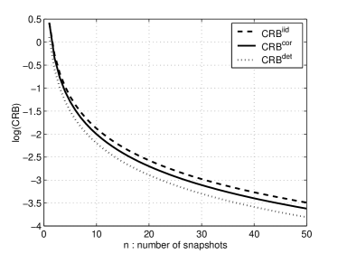
Figure 1: An example of the CRB versus the number of snapshots in logarithmic scale for two sources. The temporally correlated CRB is upper bounded by the iid CRB and lower bounded by the deterministic CRB.

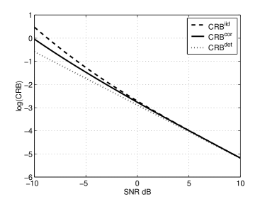
Figure 2: An example of the CRB versus the SNR in logarithmic scale for two sources. The temporally correlated CRB tends to the iid CRB as SNR increases.

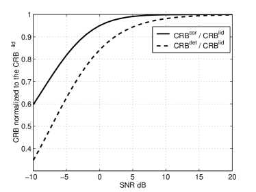
Figure 3: The comparison of the temporally correlated CRB and deterministic CRB normalized to the iid CRB. The comparison shows the equivalence of the iid and temporally correlated CRBs when SNR is high enough.

We first present some graphs on the Cramer-Rao bounds. The main result we provided on the CRBs is the inequality in (23). We also showed that the temporally correlated CRB is decreasing with the number of snapshots $n$. These facts are presented via an example of two-source scenario in Fig. 1. Conditions of the simulation are as follows: two sources at angles $[0\;\;0.2]$ radians with respect to the array broadside are present. Array number of elements is 3 with $\lambda/\,2$ spacing and SNR=10 dB. Uniform linear array is assumed and the signal covariance matrix is defined as

$$\boldsymbol{\mathcal{P}}=\boldsymbol{P}_{t}\otimes\boldsymbol{P}_{s}$$ (76)

where $[\boldsymbol{P}_{t}]_{ij}=e^{-0.2|i-j|}$, $[\boldsymbol{P}_{s}]_{ij}=e^{-0.5|i-j|}$, and $\boldsymbol{C}_{ij}=\sigma^{2}e^{-|i-j|}$. Fig. 1 shows the decreasing CRB versus increasing $n$, it also confirms the inequality in (23) for this special case. It is also noteworthy that the difference between three types of CRBs increases with $n$ since with increased number of snapshots, there are more room for the temporal correlation to improve the DOA estimation performance. In Fig. 2, CRBs are depicted versus SNR. It can be seen that as SNR increases, three types of CRB merge together and decrease linearly. Though, the $\textrm{CRB}^{\textrm{cor}}$ joins the $\textrm{CRB}^{\textrm{iid}}$ faster than $\textrm{CRB}^{\textrm{det}}$. This is better shown in Fig. 3, where the CRBs are normalized to the $\textrm{CRB}^{\textrm{iid}}$ to confirm the result of theorem 2 which is stated in (39).

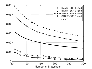
Now, we present simulation results which support the proposed method versus the main IV-SSF. In the simulations, single source located in $\omega\triangleq 2\pi\frac{d}{\lambda}\cos(\theta)=0.8$ is assumed, with a four-element half-wavelength array, number of instrumental variables $M=2$, and number of trials 10000. In Fig. 4, performance measures, bias and standard deviation of the estimate of $\omega$ are presented versus the number of snapshots $n$, while SNR=0 dB is constant. Signal temporal correlation is simulated via filtering an iid random sequence with an FIR filter with relative tap weights

$$f(z)=1+0.5z^{-1}+0.3z^{-2}+0.2z^{-3}+0.1z^{-4}$$ (77)

which is then normalized to give a unit-energy filter. The estimates are calculated using a two step grid search, first a coarse search with grid size 0.01 and then a finer one with grid size 0.001. Fig. 4 shows the bias and standard deviation of both methods versus $n$. Although bias is relatively small, it cannot be neglected in small numbers of snapshots. Although the $\textrm{CRB}^{\textrm{cor}}$ in (III) has been calculated assuming zero bias, it is still rewarding to compare the performance of the methods to the square root of the $\textrm{CRB}^{\textrm{cor}}$, which is depicted in Fig. 4. Here, we used $f(z)$ in (77) to compute the signal space-time covariance matrix $\boldsymbol{\mathcal{P}}$. The improvement made by the two-sided IV-SSF is rather constant with $n$ specially in the standard deviation. It is clear that the two-sided IV-SSF had made roughly 20% improvement in the standard deviation and bias without increasing the computational load of the algorithm.

Figure 4: Bias and standard deviation of one- and two-sided IV-SSF methods versus $n$. It is clear that the two-sided IV-SSF outperforms the one-sided one in both lower bias and lower standard deviation. The improvement is rather constant with $n$. Asymptotically in large $n$, bias is negligible in the overall mean square error.

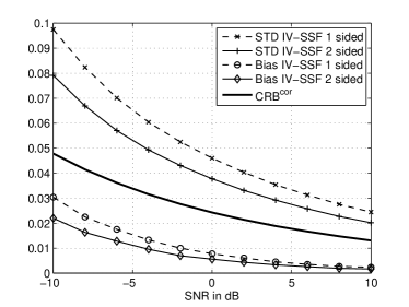
Figure 5: Bias and standard deviation of one- and two-sided IV-SSF methods versus the SNR. The improvement made by two-sided IV-SSF is larger in lower SNRs. In high SNRs, bias is negligible in the overall error.

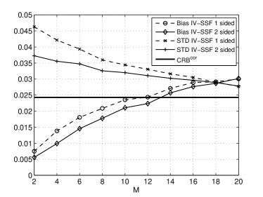
Figure 6: Bias and standard deviation of one- and two-sided IV-SSF methods versus the number of instrumental variables $M$. The improvement made by two sided IV-SSF in standard deviation is larger in low M. Also, bias grows with M and finally gets larger than standard deviation for large M.

In Fig. 5, the same comparison is made with constant $n=100$ and varying SNR. Obviously, the improvement made by two-sided IV-SSF is greater in lower SNR. In high SNR conditions, bias is rather negligible in both methods, while the improvement percentage is nearly constant with SNR. Finally in Fig. 6, the comparison is made in constant $n=100$ and SNR=0 dB, while $M$ is changed to see the effect of the method complexity indicator or the number of instrumental variables on the bias and standard deviation of both methods. The interesting point is that in low $M$, there is considerable improvement from one-sided to two-sided IV-SSF. But this improvement decreases as $M$ increases since for large $M$, there is enough previous samples to estimate the present signal of interest with sufficient accuracy comparable to the accuracy that can be achieved using the two-sided estimation. Another important point of the Fig. 6 is the increasing relative part of the bias in the overall mean square error of the estimation with increasing $M$. This phenomena can lead us to limit the number of instrumental variables so as to avoid large unpredictable bias. This selection can be more rational when we consider the increased cost of implementation when $M$ gets larger. It is also evident in Fig. 6 that the $\textrm{CRB}^{\textrm{cor}}$ is independent of $M$ and gradually, with increasing $M$, the portion of error caused by standard deviation decreases while the error caused by bias increases.

VI Conclusion

In this paper, we presented new theoretical results on the performance of the DOA estimation when signals of interest are possibly temporally correlated. In particular, it was shown that the Cramer-Rao bound in the temporally correlated signal model is upper bounded by the same bound under the iid signal model. This result implies that temporal correlation of the signals is an additional relevant information for DOA estimation. We showed that the improvement caused by signal temporal correlation is large when SNR is low and little when SNR is high. This is a good news since the high SNR condition is not critical in our systems where we can use many suboptimal methods; while the low SNR performance improvement is valuable to the system. The second part of the paper was devoted to a practical method of DOA estimation in the new signal model. The IV-SSF method was analyzed and compared with the $\textrm{CRB}^{\textrm{cor}}$ to show that it is not an efficient method. Then, using a special form of the $\textrm{CRB}^{\textrm{cor}}$, we proposed a version of the IV-SSF method (two-sided IV-SSF), that outperform the former method in both lower bias and lower error variance.

References

• [1] H. Krim and M. Viberg, “Two decades of array signal processing research: the parametric approach,” IEEE Signal Process. Mag., vol. 13, pp. 67-94, July 1996.
• [2] B. D. Van Veen and K. M. Buckley, “Beamforming: a versatile approach to spatial filtering,” IEEE ASSP Mag., pp. 4-24, Apr. 1988.
• [3] R. O. Schmidt, “Multiple emmiter location and signal parameter estimation,” IEEE Trans. Ant. Propag., vol. AP-34, pp. 276-280, March 1986.
• [4] M. Viberg and B. Ottersten, “Sensor array processing based on subspace fitting,” IEEE Trans. Signal Process., vol. 39, pp. 1110-1121, May 1991.
• [5] Y. Bresler and A. Macovski, “Exact maximum likelihood parameter estimation of superimposed exponential signals in noise,” IEEE Trans. Acoust. Speech, Signal Process., vol. ASSP-34, pp. 1081-1089, Oct. 1986.
• [6] P. Stoica and A. Nehorai, “MUSIC, maximum likelihood, and Cramer-Rao bound,” IEEE Trans. Acoust. Speech, Signal Process., vol. 37, pp. 720-741, May 1989.
• [7] X. L. Xu and K. M. Buckley, “Bias analysis of the MUSIC location estimator,” IEEE Trans. Signal Process., vol. 40, pp. 2559-2569, Oct. 1992.
• [8] P. Tichavsky, “High-SNR asymptotics for signal subspace methods in sinusoidal frequency estimation,” IEEE Trans. Signal Process., vol.41, pp. 2448-2460, July 1993.
• [9] H. Abeida and J. P. Delmas, “Gaussian Cramer-Rao bound for direction estimation of noncircular signals in unknown noise fields,” IEEE Trans. Signal Process., vol. 53, pp. 4610-4618, Dec. 2005.
• [10] A. G. Jaffer, “Maximum likelihood direction finding of stochastic sources: a separable solution,” in Proceedings International Conference Acoustic Speech Signal Processing, pp. 2893-2896, 1988.
• [11] J. P. Delmas and Y. Meurisse, “Asymptotic performance analysis of DOA finding algorithms with temporally correlated narrowband signals,” IEEE Trans. Signal Process., vol. 48, pp. 2669-2674, Sept. 2000.
• [12] M. Viberg, P. Stoica, and B. Ottersten, “Array processing in correlated noise fields based on instrumental variables and subspace fitting,” IEEE Trans. Signal Process., vol. 43, pp. 1187-1199, May 1995.
• [13] P. Stoica, M. Viberg, and B. Ottersten, “Instrumental variable approach to array processing in spatially correlated noise fields,” IEEE Trans. Signal Process., vol. 42, pp. 121-133, Jan. 1994.
• [14] P. Stoica and A. Nehorai, “Performance study of conditional and unconditional direction-of-arrival estimation,” IEEE Trans. Acoust., Speech, Signal Process., vol. 38, pp. 1783-1795, Oct. 1990.
• [15] P. Stoica, M. Viberg, M. Wong, and Q. Wu, “Optimal IV-SSF approach to array signal processing in colored noise fields,” in Proceedings of IEEE International Conference on Acoustics, speech and signal processing, pp. 2088-2091, 1995.
• [16] P. Stoica, E. G. Larsson, and A. B. Gershman, “The stochastic CRB for array processing: a textbook derivation,” IEEE Signal Process. Lett., vol. 8, pp. 148-150, May 2001.
• [17] G. Bienvenu and L. Kopp, “Optimality of high resolution array processing using the eigensystem approach,” IEEE Trans. Acoust. Speech Signal Process., vol. ASSP-31, pp. 1235-1248, Oct. 1983.
• [18] A.S. Householder, The theory of matrices in numerical analysis, Dover Publications, Newyork, 1975.