Thermally activated energy and critical magnetic fields of SmFeAsO_0.9F_0.1

Abstract

Thermally activated flux flow and vortex glass transition of recently discovered SmFeAsO_0.9F_0.1 superconductor are studied in magnetic fields up to 9.0 T. The thermally activated energy is analyzed in two analytic methods, of which one is conventional and generally used, while the other is closer to the theoretical description. The thermally activated energy values determined from both methods are discussed and compared. In addition, several critical magnetic fields determined from resistivity measurements are presented and discussed.

I Introduction

The recently discovered FeAs-based superconductors inspired study, as their superconducting transition temperatures and upper critical magnetic fields reach the values which are higher than those of MgB₂ and comparable to those of the cuprate based superconductors (CBS) Kamihara ; Ren ; Ren2 ; Wen ; Chen ; Chen2 ; Cruz ; Dong ; Hunte ; Senatore ; Jia . One of interesting characteristics is that they show layered structure with conducting layers of FeAs and charge reservoir layers of ReO, where Re is a rare earth element Ren2 . This layered structure is very similar to that of CBS, and suggests that the superconducting behaviors may have similarities to those of CBS.

The vortex dynamics of CBS have been widely studied in theories and experiments Yeshurun ; Malozemoff ; Hagen ; Geshkenbein ; Kes ; Vinokur ; Blatter ; Brandt ; Shi ; Tinkham ; Palstra ; Zhang3 ; Zhang2 ; Figueras ; Xiaowen ; Zhang ; Andersson ; Ravelosona ; Gordeev ; Yang . According to the theory, the thermally activated flux flow (TAFF) resistivity is expressed as $\rho=(2\nu_{0}LB/J)\exp(-J_{c0}BVL/T)\sinh(JBVL/T)$ Blatter ; Brandt ; Shi ; Tinkham ; Palstra , where $\nu_{0}$ is an attempt frequency for a flux bundle hopping, $L$ the hopping distance, $B$ the magnetic induction, $J$ the applied current density, $J_{c0}$ the critical current density in the absence of flux creep, $V$ the bundle volume, and $T$ the temperature. If $J$ is small enough and $JBVL/T\ll 1$, we have

$$\rho=(2\rho_{c}U/T)\exp(-U/T),$$ (1)

where $U=J_{c0}BVL$ is the thermally activated energy (TAE), and $\rho_{c}=\nu_{0}LB/J_{c0}$. Equation (1) simply means that the prefactor $2\rho_{c}U/T$ is temperature and magnetic field dependent.

Generally, the TAE of CBS is analyzed by equation (1) using an assumption that the prefactor $2\rho_{c}U/T$ is temperature independent, and $\ln\rho(H,T)$ linearly depends on $1/T$ with the form $\ln\rho(H,T)=\ln\rho_{0}(H)-U_{0}(H)/T$, where $H$ is the magnetic field strength, $\ln\rho_{0}(H)=\ln\rho_{0f}+U_{0}(H)/T_{c}$ [note that $\ln\rho_{0}(H)$ is the $\ln\rho(H)$ value for $1/T\to 0$], $\rho_{0f}$ the constant, $U_{0}$ the TAE for $T\to 0$, and $T_{c}$ the superconducting transition temperature. The importance is that the analysis leads to $U=U_{0}(1-t)$, and the apparent activate energy $-\partial\ln\rho/\partial T^{-1}=U_{0}$, where $t=T/T_{c}$ Zhang3 ; Zhang2 ; Palstra ; Figueras ; Xiaowen ; Zhang ; Andersson ; Ravelosona ; Gordeev ; Yang . By drawing resistivity data in the so-called Arrhenius plot with a relation $\ln\rho(H,1/T)$, one can easily determine $U_{0}(H)$ with its corresponding slope in a low resistivity range. However , $U=U_{0}(1-t)$ may not be true in reality, when a local slope of $\ln\rho$ vs $1/T$ in the Arrhenius plot shows a round curvature. As a result, the corresponding apparent activated energy $-\partial\ln\rho(H,T)/\partial T^{-1}$ shows a sharp increase with decreasing temperature. The phenomena means $U\neq U_{0}(1-t)$, $\rho_{0f}\neq$ const, and the determination of $U_{0}(H)$ from the slopes is a problem. In the early stage of the discovery of CBS, the experimental observation of the abnormal phenomena had been reported by Palstra et al Palstra without solution.

Zhang et al Zhang3 suggested that the temperature dependent of the prefactor in equation (1) must be taken into account in the analysis. By using this suggestion to equation (1) with $U=U_{0}(1-t)^{q}$, the derivative,

$$-\partial\ln\rho/\partial T^{-1}=(1-T/U)(U-T\partial U/\partial T)$$ (2)

$$=[U_{0}(1-t)^{q}-T][1+qt/(1-t)],$$ (3)

where $q$ has a value in the range from 0.5 to 2, and $t=T/T_{c}$.

In this paper, TAFF resistivity of SmFeAsO_0.9F_0.1 (SFAOF) is studied with magnetic fields up to 9.0 T. By using the assumption $\rho_{0f}=2\rho_{c}U/T=$ const, and $U=U_{0}(1-t)$, the TAFF behaviors were first analyzed in the Arrhenius plot. After that, by using the assumption that the prefactor $2\rho_{c}U/T$ is temperature dependent, and $\rho_{c}$ is not temperature dependent, the TAFF resistivity is analyzed in the other method in which equation (3) is employed to determine $U_{0}(H)$. The $U_{0}(H)$ determinations from both methods are discussed and compared. We suggest that the second method shall be instead of the first in the analysis of TAFF characteristics of other superconductors. In addition, the vortex glass transition, zero resistivity temperature, and the temperature dependents of the critical fields determined from different resistivity criteria values in the superconducting transition regime are presented.

II Experiments

The SFAOF sample was prepared by a high-pressure synthesis method. SmAs powder (pre-sintered) and As, Fe, Fe₂O₃, FeF₂ powders (the purities of all starting chemicals are better than 99.99%) were mixed together with the nominal stoichiometric ratio of Sm[O_1-xF_x]FeAs, then ground thoroughly and pressed into small pellets. The pellet was sealed in boron nitride crucibles and sintered in a high pressure synthesis apparatus under the pressure of 6.0 GPa and temperature of 1250^∘ C for two hours. The x-ray diffraction analysis showed that the main phase is LaOFeAs structure with some impurity phases Ren ; Ren2 . It was cut into a rectangular shape with dimensions of 4.20 mm(length)$\times$ 1.60 mm(width) $\times$ 1.08 mm(thickness). The standard four probe technique was used for resistivity $\rho(T,H)$ measurements. Bipolar pulsed dc current with an amplitude of 5.0 mA (corresponding to the current density about $\sim$0.29 A/cm²) was applied to it. The measurements were performed on a physical property measurement system (PPMS, Quantum Design) with the magnetic field up to 9 T. From the zero field $\rho(T,0)$ data, we find that the superconducting transition width is about 1.7 K (defined by the superconducting transition from 10% to 90% of the normal resistivity), and the zero resistant temperature $T_{c0}$ is 52.2 K (determined by the criterion of 0.1 ${\mu\Omega\cdot}$cm).

III Results and discussion

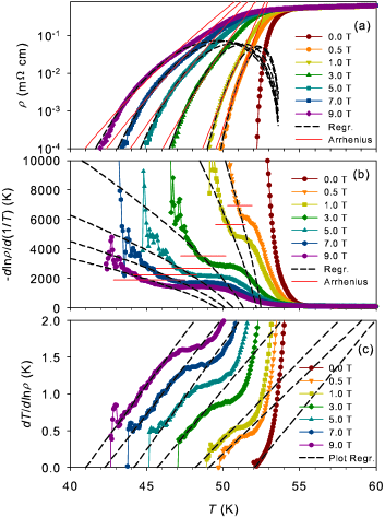
Figure 1: (a)-(c), respectively, show $\rho(T,H)$, $-\partial\ln\rho(T,H)/\partial T^{-1}$, and $\partial T/\partial\ln\rho(T,H)$ data in magnetic fields of $\mu_{0}H=0.0$, 0.5, 1.0, 3.0, 5.0, 7.0, and 9.0 T with different symbols. The solid lines in (a) and short horizontal lines in (b) correspond to the regressions with the fitting parameters of $U_{0}(H)$ and $\rho_{0f}$ determined from the first analytic method. The dashed lines are regression curves with the fitting parameters $U_{0}(H)$ and $\rho_{c}(H)$ determinded from the second analytic method (see text). The dashed lines in (c) plot linear fittings.

Figure 1(a)-(c), respectively, show $\rho(T,H)$, $-\partial\ln\rho(T,H)/\partial T^{-1}$, and $\partial T/\ln\rho(T,H)$ data with different symbols for 0.0, 0.5, 1.0, 3.0, 5.0, 7.0, and 9.0 T fields. One shall notice that the suppression of the superconductivity at 9.0 T field is comparable to that of low anisotropic CBS, e.g. YBa₂Cu₃O_7-δ (YBCO), and suggests that the anisotropy is similar to YBCO. The so-called apparent activated energy $-\partial\ln\rho(T,H)/\partial T^{-1}$ data were generally used to analyze TAE Palstra ; Zhang3 , and the derivative $\partial T/\ln\rho(T,H)$ data is always used to analysis the vortex glass transition boundary Fisher ; Fisher2 ; Wagner ; Zhang1 . Below, we will present our analysis.

Figure 2: Arrhenius plot of $\rho(T,H)$ for $\mu_{0}H=0.0$, 0.5, 1.0, 3.0, 5.0, 7.0, and 9.0 T. The solid lines are plot linear fitting for low resistivity. The dashed lines are regressive curves using the second analytic method. The inset shows $\ln\rho_{0}(U_{0})$ data determined by using the first analytic method, where the solid line is a linear fit for the data.

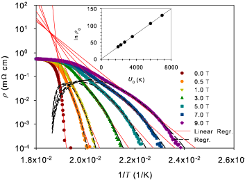
Figure 2 shows the Arrhenius plot of its resistivity in magnetic fields of $\mu_{0}H=0.0$, 0.5, 1.0, 3.0, 5.0, 7.0, and 9.0 T with different symbols. The solid lines plot linear regressions in the low resistivity range. According to the conventional analysis method, these linear fits are based on the assumption $U(T,H)=U_{0}(H)(1-t)$, where each $U_{0}(H)$ was determined by using each slope. Note that there is a cross point where all the linear fitting lines approximately focus together except for the line for zero field, and this point leads to $T_{cr}\approx 53.8$ K. The inset shows $\ln\rho_{0}(U_{0})$ data and the corresponding solid line with the linear fitting $\ln\rho_{0}=\ln\rho_{0f}+U_{0}/T_{c}$. From the fitting, we determined $\rho_{0f}=6.668$ m$\Omega\cdot$cm, and $T_{c}\approx 53.8$ K which coincides with the value of $T_{cr}$. Using the $\rho_{0f}$, $T_{c}$, and $U_{0}(H)$ data, we regressed the $\rho(T,H)$ data as shown in figure 1(a) with solid lines. Since the assumption of $U(T,H)=U_{0}(H)(1-t)$ leads to $-\partial\ln\rho(T,H)/\partial T^{-1}=U_{0}$, we present $U_{0}(H)$ data in figure 1(b) with horizontal solid lines where each of them has a limited length. Each length covers the temperature interval which corresponds to the interval of the reciprocal temperature for determining $U_{0}(H)$ in the Arrhenius plot. For decreasing temperature, note that each $-\partial\ln\rho(T,H)/\partial T^{-1}$ dataset approximately intersects its horizontal $U_{0}(H)$ line center with a divergent trend in the temperature interval. This means that each $U_{0}(H)$ approximates to the average value of its $-\partial\ln\rho(T,H)/\partial T^{-1}$ in the temperature interval. The similar divergent trends were also observed in YBCO Palstra ; Zhang3 . The analysis indicates that the TAE determined from the conventional method may have problems in characteristics, and the method suggested by Zhang et al Zhang3 ought to be taken into consideration.

In figure 1(b), one may have noticed that each $-\partial\ln\rho(T,H)/\partial T^{-1}$ set can be divided into five regimes: (i) the normal state regime at high temperature, where $-\partial\ln\rho(T,H)/\partial T^{-1}$ is almost temperature-and magnetic-field-independent; (ii) the primary superconducting transition regime, where $-\partial\ln\rho(T,H)/\partial T^{-1}$ quickly increases and the resistivity begins sharply decreasing (see figure 1(a)); (iii) the platform regime, where $-\partial\ln\rho(T,H)/\partial T^{-1}$ for each field measurement show a step structure (see figure 1(b)); (iv) the second sharply increasing regime, where $-\partial\ln\rho(T,H)/\partial T^{-1}$ quickly increases into a high value range and $\partial T/\partial\ln\rho$ data show a linear type (see figure 1(c)); (v) the strong fluctuation regime, where $-\partial\ln\rho(T,H)/\partial T^{-1}$ curve shows an irregular shape due to the resistivity reaching the low measurable range.

For analyzing TAFF behaviors with the second analytic method, the first thing is to validate one or two regimes which relate to the TAFF behaviors. Apparently, the data in regimes (i) and (ii) do not relate to TAFF behaviors, as the data are in the normal state in regime (i) and in the flux flow regime in regime (ii). The data show a platform structure and possibly relate to TAFF behaviors in regime (iii). Note that resistivity data in the regime are only about one order of magnitude less than that in regime (i) (where the resistivity is in the normal state) [see figure 1(a) and (b)]. Therefore, we conclude that the data in regime (iii) are not in the TAFF regime Palstra . In regime (iv), the resistivity is about 2 and 3 orders of magnitude less than that in regime (i). The resistivity in this range, as suggested by Palstra et al Palstra , relates to TAFF behavior. According to the vortex glass transition theory, the linear (ohmic) resistivity ought to linearly vanish in a form $\rho\propto(T-T_{g})$, where $T_{g}$ is the vortex glass transition temperature Fisher ; Fisher2 . Accordingly, $\partial T/\partial\ln\rho\propto(T-T_{g})$ Wagner ; Zhang1 . In figure 1(b), one will easily find that $\partial T/\partial\ln\rho(T,H)$ curves show approximately linear curvatures in regime (iv). The data in the regime (v) show irregular trend, as the resistivity is going to a deeply superconducting state where the resistivity may be dominated by non-ohmic characteristics; besides, the measuring voltmeter reached its low measuring limitation in experiments. The analysis concludes that the TAFF resistivity is in regime (iv).

Figure 3 shows $U_{0}(H)$ determined by the first analytic method with circles and by the second with triangles. The stars show corresponding $\rho_{c}(H)$ for the second method. All the dash lines in figures 1(a) and (b), and figure 2 are regression curves with the regression parameters of $U_{0}(H)$ and $\rho_{c}(H)$ in figure 3. In the analysis of these data with the second method, we first derived $U_{0}$ with equation (3) as $U_{0}$ is the only free parameter in the equation except for $q$. We found that the energy relation, $U(T,H)=U_{0}(1-t)^{q}$ with $q=2$, leads to good consistency to the experimental data, where $t=T/T_{c}$, and $T_{c}=53.8$ K. After determination of each $U_{0}(H)$, each $\rho_{c}(H)$ can be easily determined by fitting equation (1). One will find that all the regressions (dashed lines) in figure 1(a), figure 1(b), and figure 2 are in good agreement with experimental data and confirm the correctness of the analytic method. Note that, although each temperature interval in regime (iv), which we used to determine $U_{0}(H)$ with the second analytic method, is somewhat less than that we used to determine $U_{0}(H)$ with the first analytic method (see figure 1(b) and (c)), the regressions of the second method are still given better fitting results.

Figure 3: (a) The circles show $U_{0}(H)$ extracted from the slopes in Arrhenius plot in figure 2. The downward triangles show $U_{0}(H)$ data determined by using the relation $-\partial\ln\rho/\partial T^{-1}=[U_{0}(1-t)^{q}-T][1+qt/(1-t)]$, where $q=2$. The stars represent corresponding $\rho_{c}$ data.

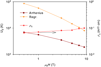
For magnetic field above 1.0 T, we find that $U\propto H^{-0.57}(1-t)$ for the data derived from Arrhenius plot with the first method, and $U\propto H^{-0.99}(1-t)^{2}$ with the second method. Note that the TAE determined by the second method is about one order larger than that determined from the first as shown in the figure. The reason of the large difference between the two analytic methods is due to that the first method not taking into account the temperature dependent relation of the prefactor in equation (1), while the second method takes into consideration. Apparently, the second method is closer to the theoretical description.

Figure 4: Critical magnetic fields. The circles show the $H(T_{g})$ data, the downward triangles the $H(T_{c0})$, the squares the $H(T_{10\%})$, the diamonds the $H(T_{50\%})$, and the upward triangles the $H(T_{90\%})$.

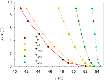
Figure 4 shows the vortex glass transition boundary $H(T_{g})$, $H(T_{c0})$, $H(T_{10\%})$, $H(T_{50\%})$, and $H(T_{90\%})$,where $T_{g}$ is the glass transition temperature, $T_{c0}$ the zero resistance temperature, $T_{10\%}$ the 10% of the normal state resistivity temperature, $T_{50\%}$ the 50% and $T_{90\%}$ the 90%. Here, $H(T_{g})$ was determined by using the $\partial T/\partial\ln\rho\propto(T-T_{g})$ relation [dash lines in figure 2(c)]. We find that the data can be fitted by a relation $H_{g}=H_{g0}(1-T_{g}/52.05)^{2}$, where $\mu_{0}H_{g0}\approx 201$ T. The $\mu_{0}H_{g0}$ value may not be true in zero temperature, but it leads to a conclusion that the vortex melting field is very large for SFAOF superconductor when the temperature approaches to zero. A similar characteristic can be also observed for $H(T_{c0})$ data, since each $T_{c0}(H)$ is slightly higher than that $T_{g}(H)$. The normalized transition widths (defined as $(1-T_{10\%}/T_{90\%})$ are comparable to YBCO, and thus suggest that the anisotropy of the SFAOF is similar to YBCO. The $H(T_{90\%})$ curve shows a steep increase indicating that the upper critical magnetic field of the superconductor is very high in low temperature. One may notice that the transition widths between $T_{c0}(H)$ and $T_{10\%}(H)$ are comparable to that between $T_{10\%}(H)$ and $T_{90\%}(H)$, suggesting that superconductor may have better analysis results when further improving the quality of the superconductor.

In comparisons, a sample that was prepared in the same sample batch was used in ac susceptibility measurements with magnetic fields up to 7.0 T, and frequencies up to 1.11 kHz. We found that $T_{g}(H)$ is somewhat larger than the corresponding temperature of the peak in the imaginary component in ac susceptibility measurement. However, the similar $H$ increasing trends were also found in the ac measurement. Besides, we found that the onset temperature of the superconducting transition $T_{onset}(H)$ of ac susceptibility measurement is somewhat higher than that of $T_{c0}(H)$. Detailed analysis of the ac measurement is just ongoing.

IV Conclusion

In summary, we analyze the resistive TAFF behavior of SFAOF with two theoretical analysis. For the first method, $\rho_{0f}=$ const and $U=U_{0}(1-t)$ were assumed, and thus Arrhenius plot was employed in analysis. This method is simple and easy in analysis, but the analysis results remain inconsistency to experimental data. The second method assumes that the prefactor $2\rho_{c}U/T$ is temperature dependent, while $\rho_{c}$ is not temperature dependent. By using the second method, equation (3) is obtained. The second method results in the regressions are in good agreement with experimental data. The TAE analysis shows $U\sim H^{-1}(1-t)^{2}$ for magnetic field above 1.0 T. The second method is also simple and easy, since only two free parameters in analysis. We suggest that the second method shall be instead of the first for the analysis of TAFF behaviors of other superconductors. The study shows that critical magnetic fields of SFAOF may have large values in low temperature and comparable to CBS.

V Acknowledgements

We are grateful to Prof. H. H. Wen and Dr. H. Yang for resistivity measurements and helpful discussion. This work has been financially supported by the National Natural Science Foundation of China (Grant No. 10874221).

References

- (1) Y. Kamihara, T. Watanabe, M. Hirano, and H. Hosono, J. Am. Chem. Soc. 130, 3296 (2008).
- (2) Z. A. Ren, W. Lu, J. Yang, W. Yi, X. L. Shen, Z. C. Li, G. C. Che, X. L. Dong, L. L. Sun, F. Zhou, and Z. X. Zhao, Chin. Phys. Lett. 25, 2215 (2008).
- (3) Z. A. Ren, G. C. Che, X. L. Dong, J. Yang, W. Lu, W. Yi, X. L. Shen, Z. C. Li, L. L. Sun, F. Zhou, Z. X. Zhao, Europhysics Letters 83, 17002 (2008).
- (4) H. H. Wen, G. Mu, L. Fang, H. Yang, and X. Zhu, Europhys. Lett. 82, 17009 (2008).
- (5) G. F. Chen, Z. Li, D. Wu, G. Li, W. Z. Hu, J. Dong, P. Zheng, J. L. Luo, N. L. Wang , Phys. Rev. Lett. 100, 247002 (2008).
- (6) G. F. Chen, Z. Li, D. Wu, J. Dong, G. Li, W. Z. Hu, P. Zheng, J. L. Luo, N. L. Wang, Chin. Phys. Lett. 25, 2235 (2008).
- (7) Clarina de la Cruz, Q. Huang, J. W. Lynn, Jiying Li, W. Ratcliff II, J. L. Zarestky, H. A. Mook, G. F. Chen, J. L. Luo, N. L. Wang, Pengcheng Dai, Nature 453, 899 (2008).
- (8) J. Dong, H. J. Zhang, G. Xu, Z. Li, G. Li, W. Z. Hu, D. Wu, G. F. Chen, X. Dai, J. L. Luo, Z. Fang, N. L. Wang, Europhysics Letters, 83, 27006 (2008).
- (9) F. Hunte, J. Jaroszynski, A. Gurevich, D. C. Larbalestier, R. Jin, A. S. Sefat, M. A. McGuire, B. C. Sales, D. K. Christen, and D. Mandrus, Nature (London) 453, 903 (2008).
- (10) C. Senatore, M. Cantoni, G. Wu, R.H. Liu, X.H. Chen, and R. Flükiger, arXiv:0805.2389.
- (11) Y. Jia, P. Cheng, L. Fang, H. Q. Luo, H. Yang, C. Ren, L. Shan, C. Z. Gu, and H. H. Wen, arXiv:0806.0532.
- (12) Y. Yeshurun and A. P. Malozemoff, Phys. Rev. Lett. 60, 2202 (1988).
- (13) A. P. Malozemoff, L. Krusin-Elbaum, D. C. Cronemeyer, Y. Yeshurun and F. Holtzberg, Phys. Rev. B 38, 6490 (1988).
- (14) C. W. Hagen and R. Griessen, Phys. Rev. Lett. 62, 2857 (1989).
- (15) V. B. Geshkenbein, M. V. Feigel’man, A. I. Larkin, and V. M. Vinokur, Physica C 162, 239 (1989).
- (16) P. H. Kes, J. Aarts, .J van den Berg, C. J. van der Beek and J. A. Mydosh, Supercond. Sci. Technol. 1, 242 (1989).
- (17) V. M. Vinokur, M. V. Feigel’man, V. B. Geshkenbein, and A. I. Larkin, Phys. Rev. Lett. 65, 259 (1990); J. Kierfeld, H. Nordborg, and V. M. Vinokur, Phys. Rev. Lett. 85, 4948 (2000).
- (18) G. Blatter, M. V. Feigel’man, V. B. Geshkenbein, A. I. Larkin, and V. M. Vinokur, Rev. Mod. Phys. 66, 1125 (1994), (and the references therein).
- (19) E. H. Brandt, Rep. Prog. Phys. 58, 1465 (1995), (and the references therein).
- (20) D. Shi, High-Temperature Superconducting Materials Science and Engineering New Concepts and Technology, (Pergamon, New York, 1995).
- (21) M. Tinkham, Introduct. to Superconduct., McGraw-Hill, New York, 1996, (and the references therein).
- (22) T. T. M. Palstra, B. Batlogg, L. F. Schneemeyer and J. V. Waszczak, Phys. Rev. Lett. 61, 1662 (1988); T. T. M. Palstra, B. Batlogg, R. B. van Dover, I. F. Schneemeyer, and J. V. Waszczak, Phys. Rev. B 41, 6621 (1990).
- (23) Y. Z. Zhang, H. H. Wen, Z. Wang, Phys. Rev. B 74, 144521 (2006).
- (24) Y. Z. Zhang, Z. Wang, X. F. Lu, H. H. Wen, J. F. de Marneffe, R. Deltour, A. G. M. Jansen, and P. Wyder, Phys. Rev. B 71, 052502 (2005).
- (25) J. Figueras, T. Puig, and X. Obradors Phys. Rev. B 67, 014503 (2003)
- (26) Cao Xiaowen, Wang Zhihe, and Xu Xiaojun Phys. Rev. B 65, 064521 (2002); Xu Xiaojun, Fu Lan, Wang Liangbin, Zhang Yuheng, Fang Jun, Cao Xiaowen, Li Kebin, and Sekine Hisashi Phys. Rev. B 59, 608 (1999).
- (27) Y. Z. Zhang, R. Deltour, and Z. X. Zhao, Phys. Rev. Lett. 85, 3492 (2000).
- (28) M. Andersson, A. Rydh, and Ö. Rapp Phys. Rev. B 63, 184511 (2001).
- (29) D. Ravelosona, J. P. Contour, and N. Bontemps Phys. Rev. B 61, 7044 (2000).
- (30) S. N. Gordeev, A. P. Rassau, R. M. Langan, P. A. J. de Groot, V. B. Geshkenbein, R. Gagnon, and L. Taillefer Phys. Rev. B 60, 10477 (1999).
- (31) H. C. Yang, L. M. Wang, and H. E. Horng Phys. Rev. B 59, 8956 (1999).
- (32) M.P.A. Fisher, Phys. Rev. Lett. 62, 1415 (1989).
- (33) D.S. Fisher, M.P.A. Fisher, and D.A. Huse, Phys. Rev. B 43, 130 (1991).
- (34) P. Wagner, U. Frey, F. Hillmer, and H. Adrian, Phys. Rev. B 51, 1206 (1995).
- (35) Y. Z. Zhang, R. Deltour, J.-F. de Marneffe, Y. L. Qin, L. Li, Z. X. Zhao, A. G. M. Jansen, and P. Wyder Phys. Rev. B 61, 8675 (2000).