NESTA: A Fast and Accurate First-order Method
for Sparse Recovery

Abstract

Accurate signal recovery or image reconstruction from indirect and possibly undersampled data is a topic of considerable interest; for example, the literature in the recent field of compressed sensing is already quite immense. Inspired by recent breakthroughs in the development of novel first-order methods in convex optimization, most notably Nesterov’s smoothing technique, this paper introduces a fast and accurate algorithm for solving common recovery problems in signal processing. In the spirit of Nesterov’s work, one of the key ideas of this algorithm is a subtle averaging of sequences of iterates, which has been shown to improve the convergence properties of standard gradient-descent algorithms. This paper demonstrates that this approach is ideally suited for solving large-scale compressed sensing reconstruction problems as 1) it is computationally efficient, 2) it is accurate and returns solutions with several correct digits, 3) it is flexible and amenable to many kinds of reconstruction problems, and 4) it is robust in the sense that its excellent performance across a wide range of problems does not depend on the fine tuning of several parameters. Comprehensive numerical experiments on realistic signals exhibiting a large dynamic range show that this algorithm compares favorably with recently proposed state-of-the-art methods. We also apply the algorithm to solve other problems for which there are fewer alternatives, such as total-variation minimization, and convex programs seeking to minimize the $\ell_{1}$ norm of $Wx$ under constraints, in which $W$ is not diagonal.

1 Introduction

Compressed sensing (CS) [13, 14, 25] is a novel sampling theory, which is based on the revelation that one can exploit sparsity or compressibility when acquiring signals of general interest. In a nutshell, compressed sensing designs nonadaptive sampling techniques that condense the information in a compressible signal into a small amount of data. There are some indications that because of the significant reduction in the number of measurements needed to recover a signal accurately, engineers are changing the way they think about signal acquisition in areas ranging from analog-to-digital conversion [23], digital optics, magnetic resonance imaging [38], seismics [37] and astronomy [8].

In this field, a signal $x^{0}\in\mathbb{R}^{n}$ is acquired by collecting data of the form

$$b=Ax^{0}+z,$$

where $x^{0}$ is the signal of interest (or its coefficient sequence in a representation where it is assumed to be fairly sparse), $A$ is a known $m\times n$ “sampling” matrix, and $z$ is a noise term. In compressed sensing and elsewhere, a standard approach attempts to reconstruct $x^{0}$ by solving

$$\begin{array}[]{ll}\text{minimize}&\quad f(x)\\ \text{subject to}&\quad\|b-Ax\|_{\ell_{2}}\leq\epsilon,\end{array}$$ (1)

where $\epsilon^{2}$ is an estimated upper bound on the noise power. The choice of the regularizing function $f$ depends on prior assumptions about the signal $x^{0}$ of interest: if $x^{0}$ is (approximately) sparse, an appropriate convex function is the $\ell_{1}$ norm (as advocated by the CS theory); if $x^{0}$ is a piecewise constant object, the total-variation norm provides accurate recovery results, and so on.

Solving large-scale problems such as (1) (think of $x^{0}$ as having millions of entries as in mega-pixel images) is challenging. Although one cannot review the vast literature on this subject, the majority of the algorithms that have been proposed are unable to solve these problems accurately with low computational complexity. On the one hand, standard second-order methods such as interior-point methods [10, 36, 48] are accurate but problematic for they need to solve large systems of linear equations to compute the Newton steps. On the other hand, inspired by iterative thresholding ideas [24, 30, 20], we have now available a great number of first-order methods, see [31, 9, 34, 35] and the many earlier references therein, which may be faster but not necessarily accurate. Indeed, these methods are shown to converge slowly, and typically need a very large number of iterations when high accuracy is required.

We would like to pause on the demand for high accuracy since this is the main motivation of the present paper. While in some applications, one may be content with one or two digits of accuracy, there are situations in which this is simply unacceptable. Imagine that the matrix $A$ models a device giving information about the signal $x^{0}$, such as an analog-to-digital converter, for example. Here, the ability to detect and recover low-power signals that are barely above the noise floor, and possibly further obscured by large interferers, is critical to many applications. In mathematical terms, one could have a superposition of high power signals corresponding to components $x^{0}[i]$ of $x^{0}$ with magnitude of order 1, and low power signals with amplitudes as far as 100 dB down, corresponding to components with magnitude about $10^{-5}$. In this regime of high-dynamic range, very high accuracy is required. In the example above, one would need at least five digits of precision as otherwise, the low power signals would go undetected.

Another motivation is solving (1) accurately when the signal $x^{0}$ is not exactly sparse, but rather approximately sparse, as in the case of real-world compressible signals. Since exactly sparse signals are rarely found in applications—while compressible signals are ubiquitous—it is important to have an accurate first-order method to handle realistic signals.

1.1 Contributions

A few years ago, Nesterov [43] published a seminal paper which couples smoothing techniques (see [4] and the references therein) with an improved gradient method to derive first-order methods which achieve a convergence rate he had proved to be optimal [41] two decades earlier. As a consequence of this breakthrough, a few recent works have followed up with improved techniques for some very special problems in signal or image processing, see [3, 21, 52, 1] for example, or for minimizing composite functions such as $\ell_{1}$-regularized least-squares problems [44]. In truth, these novel algorithms demonstrate great promise; they are fast, accurate and robust in the sense that their performance does not depend on the fine tuning of various controlling parameters.

This paper also builds upon Nesterov’s work by extending some of his works discussed just above, and proposes an algorithm—or, better said, a class of algorithms—for solving recovery problems from incomplete measurements. We refer to this algorithm as NESTA—a shorthand for Nesterov’s algorithm—to acknowledge the fact that it is based on his method. The main purpose and the contribution of this paper consist in showing that NESTA obeys the following desirable properties.

1. Speed: NESTA is an iterative algorithm where each iteration is decomposed into three steps, each involving only a few matrix-vector operations when $A^{*}A$ is an orthogonal projector and, more generally, when the eigenvalues of $A^{*}A$ are well clustered. This, together with the accelerated convergence rate of Nesterov’s algorithm [43, 3], makes NESTA a method of choice for solving large-scale problems. Furthermore, NESTA’s convergence is mainly driven by a single smoothing parameter $\mu$ introduced in Section 2. One can use continuation techniques [34, 35] to dynamically update this parameter to substantially accelerate this algorithm.

2. Accuracy: NESTA depends on a few parameters that can be set in a very natural fashion. In fact, there is a trivial relationship between the value of these parameters and the desired accuracy. Furthermore, our numerical experiments demonstrate that NESTA can find the first 4 or 5 significant digits of the optimal solution to (1), where $f(x)$ is the $\ell_{1}$ norm or the total-variation norm of $x$, in a few hundred iterations. This makes NESTA amenable to solve recovery problems involving signals of very large sizes that also exhibit a great dynamic range.

3. Flexibility: NESTA can be adapted to solve many problems beyond $\ell_{1}$ minimization with the same efficiency, such as total-variation (TV) minimization problems. In this paper, we will also discuss applications in which $f$ in (1) is given by $f(x)=\|Wx\|_{\ell_{1}}$, where one may think of $W$ as a short-time Fourier transform also known as the Gabor transform, a curvelet transform, an undecimated wavelet transform and so on, or a combination of these, or a general arbitrary dictionary of waveforms (note that this class of recovery problems also include weighted $\ell_{1}$ methods [16]). This is particularly interesting because recent work [29] suggests the potential advantage of this analysis-based approach over the classical basis pursuit in solving important inverse problems [29].

A consequence of these properties is that NESTA, and more generally Nesterov’s method, may be of interest to researchers working in the broad area of signal recovery from indirect and/or undersampled data.

Another contribution of this paper is that it also features a fairly wide range of numerical experiments comparing various methods against problems involving realistic and challenging data. By challenging, we mean problems of very large scale where the unknown solution exhibits a large dynamic range; that is, problems for which classical second-order methods are too slow, and for which standard first-order methods do not provide sufficient accuracy. More specifically, Section 5 presents a comprehensive series of numerical experiments which illustrate the behavior of several state-of-the-art methods including interior point methods [36], projected gradient techniques [34, 51, 31], fixed point continuation and iterative thresholding algorithms [34, 56, 3]. It is important to consider that most of these methods have been perfected after several years of research [36, 31], and did not exist two years ago. For example, the Fixed Point Continuation method with Active Set [35], which represents a notable improvement over existing ideas, was released while we were working on this paper.

1.2 Organization of the paper and notations

As emphasized earlier, NESTA is based on Nesterov’s ideas and Section 2 gives a brief but essential description of Nesterov’s algorithmic framework. The proposed algorithm is introduced in Section 3. Inspired by continuation-like schemes, an accelerated version of NESTA is described in Section 3.6. We report on extensive and comparative numerical experiments in Section 5. Section 6 covers extensions of NESTA to minimize the $\ell_{1}$ norm of $Wx$ under data constraints (Section 6.1), and includes realistic simulations in the field of radar pulse detection and estimation. Section 6.3 extends NESTA to solve total-variation problems and presents numerical experiments which also demonstrate its remarkable efficiency there as well. Finally, we conclude with Section 7 discussing further extensions, which would address an even wider range of linear inverse problems.

Notations. Before we begin, it is best to provide a brief summary of the notations used throughout the paper. As usual, vectors are written in small letters and matrices in capital letters. The $i$th entry of a vector $x$ is denoted $x[i]$ and the $(i,j)$th entry of the matrix $A$ is $A[i,j]$.

It is convenient to introduce some common optimization problems that will be discussed throughout. Solving sparse reconstruction problems can be approached via several different equivalent formulations. In this paper, we particularly emphasize the quadratically constrained $\ell_{1}$-minimization problem

$$\begin{array}[]{lll}(\text{BP}_{\epsilon})&\quad\text{minimize}&\quad\|x\|_{\ell_{1}}\\ &\quad\text{subject to}&\quad\|b-Ax\|_{\ell_{2}}\leq\epsilon,\end{array}$$ (2)

where $\epsilon$ quantifies the uncertainty about the measurements $b$ as in the situation where the measurements are noisy. This formulation is often preferred because a reasonable estimate of $\epsilon$ may be known. A second frequently discussed approach considers solving this problem in Lagrangian form, i.e.

$$(\text{QP}_{\lambda})\quad\text{minimize}\quad\lambda\|x\|_{\ell_{1}}+\frac{1}{2}\|b-Ax\|_{\ell_{2}}^{2},$$ (3)

and is also known as the basis pursuit denoising problem (BPDN) [18]. This problem is popular in signal and image processing because of its loose interpretation as a maximum a posteriori estimate in a Bayesian setting. In statistics, the same problem is more well-known as the lasso [49]

$$\begin{array}[]{lll}(\text{LS}_{\tau})&\quad\text{minimize}&\quad\|b-Ax\|_{\ell_{2}}\\ &\quad\text{subject to}&\quad\|x\|_{\ell_{1}}\leq\tau.\end{array}$$ (4)

Standard optimization theory [47] asserts that these three problems are of course equivalent provided that $\epsilon,\lambda,\tau$ obey some special relationships. With the exception of the case where the matrix $A$ is orthogonal, this functional dependence is hard to compute [51]. Because it is usually more natural to determine an appropriate $\epsilon$ rather than an appropriate $\lambda$ or $\tau$, the fact that NESTA solves ($\text{BP}_{\epsilon}$) is a significant advantage. Further, note that theoretical equivalence of course does not mean that all three problems are just as easy (or just as hard) to solve. For instance, the constrained problem ($\text{BP}_{\epsilon}$) is harder to solve than ($\text{QP}_{\lambda}$), as discussed in Section 5.2. Therefore, the fact that NESTA turns out to be competitive with algorithms that only solve ($\text{QP}_{\lambda}$) is quite remarkable.

2 Nesterov’s method

2.1 Minimizing smooth convex functions

In [42, 41], Nesterov introduces a subtle algorithm to minimize any smooth convex function $f$ on the convex set $\mathcal{Q}_{p}$,

$$\min_{x\in\mathcal{Q}_{p}}f(x).$$ (5)

We will refer to $\mathcal{Q}_{p}$ as the primal feasible set. The function $f$ is assumed to be differentiable and its gradient $\nabla f(x)$ is Lipschitz and obeys

$$||\nabla f(x)-\nabla f(y)||_{\ell_{2}}\leq L\|x-y\|_{\ell_{2}};$$ (6)

in short, $L$ is an upper bound on the Lipschitz constant. With these assumptions, Nesterov’s algorithm minimizes $f$ over $\mathcal{Q}_{p}$ by iteratively estimating three sequences $\{x_{k}\}$, $\{y_{k}\}$ and $\{z_{k}\}$ while smoothing the feasible set $\mathcal{Q}_{p}$. The algorithm depends on two scalar sequences $\{\alpha_{k}\}$ and $\{\tau_{k}\}$ discussed below, and takes the following form:

Initialize $x_{0}$. For $k\geq 0$, 1. Compute $\nabla f(x_{k})$. 2. Compute $y_{k}$: $y_{k}\!=\!\mathop{\mbox{argmin}}_{x\in Q_{p}}\frac{L}{2}\|x-x_{k}\|_{\ell_{2}}^{2}+\langle\nabla f(x_{k}),x-x_{k}\rangle$. 3. Compute $z_{k}$: $z_{k}\!=\!\mathop{\mbox{argmin}}_{x\in Q_{p}}\frac{L}{\sigma_{p}}p_{p}(x)+\sum_{i=0}^{k}\alpha_{i}\langle\nabla f(x_{i}),x-x_{i}\rangle$. 4. Update $x_{k}$: $x_{k}\!=\!\tau_{k}z_{k}+(1-\tau_{k})y_{k}$. Stop when a given criterion is valid.

At step $k$, $y_{k}$ is the current guess of the optimal solution. If we only performed the second step of the algorithm with $y_{k-1}$ instead of $x_{k}$, we would obtain a standard first-order technique with convergence rate $\mathcal{O}(1/k)$.

The novelty is that the sequence $z_{k}$ “keeps in mind” the previous iterations since Step 3 involves a weighted sum of already computed gradients. Another aspect of this step is that—borrowing ideas from smoothing techniques in optimization [4]—it makes use of a prox-function $p_{p}(x)$ for the primal feasible set $Q_{p}$. This function is strongly convex with parameter $\sigma_{p}$; assuming that $p_{p}(x)$ vanishes at the prox-center $x_{p}^{c}=\mathop{\mbox{argmin}}_{x}p_{p}(x)$, this gives

$$p_{p}(x)\geq\frac{\sigma_{p}}{2}\|x-x_{p}^{c}\|_{\ell_{2}}^{2}.$$

The prox-function is usually chosen so that $x_{p}^{c}\in\mathcal{Q}_{p}$, thus discouraging $z_{k}$ from moving too far away from the center $x_{p}^{c}$.

The point $x_{k}$, at which the gradient of $f$ is evaluated, is a weighted average between $z_{k}$ and $y_{k}$. In truth, this is motivated by a theoretical analysis [43, 50], which shows that if $\alpha_{k}=1/2(k+1)$ and $\tau_{k}=2/(k+3)$, then the algorithm converges to

$$x^{\star}=\mathop{\mbox{argmin}}_{x_{\in}Q_{p}}f(x)$$

with the convergence rate

$$f(y_{k})-f(x^{\star})\leq\frac{4Lp_{p}(x^{\star})}{(k+1)^{2}\sigma_{p}}.$$ (7)

This decay is far better than what is achievable via standard gradient-based optimization techniques since we have an approximation scaling like $L/k^{2}$ instead of $L/k$.

2.2 Minimizing nonsmooth convex functions

In an innovative paper [43], Nesterov recently extended this framework to deal with nonsmooth convex functions. Assume that $f$ can be written as

$$f(x)=\max_{u\in\mathcal{Q}_{d}}\langle u,Wx\rangle,$$ (8)

where $x\in\mathbb{R}^{n}$, $u\in\mathbb{R}^{p}$ and $W\in\mathbb{R}^{p\times n}$. We will refer to $\mathcal{Q}_{d}$ as the dual feasible set, and suppose it is convex. This assumption holds for all of the problems of interest in this paper—we will see in Section 3 that this holds for $\|x\|_{\ell_{1}}$, $\|Wx\|_{\ell_{1}}$, the total-variation norm and, in general, for any induced norm—yet it provides enough information beyond the black-box model to allow cleverly-designed methods with a convergence rate scaling like $\mathcal{O}(1/k^{2})$ rather than $\mathcal{O}(1/\sqrt{k})$, in the number of steps $k$.

With this formulation, the minimization (5) can be recast as the following saddle point problem:

$$\min_{x\in\mathcal{Q}_{p}}\max_{u\in\mathcal{Q}_{d}}\langle u,Wx\rangle.$$ (9)

The point is that $f$ (8) is convex but generally nonsmooth. In [43], Nesterov proposed substituting $f$ by the smooth approximation

$$f_{\mu}(x)=\max_{u\in\mathcal{Q}_{d}}\langle u,Wx\rangle-\mu\,p_{d}(u),$$ (10)

where $p_{d}(u)$ is a prox-function for $\mathcal{Q}_{d}$; that is, $p_{d}(u)$ is continuous and strongly convex on $\mathcal{Q}_{d}$, with convexity parameter $\sigma_{d}$ (we shall assume that $p_{d}$ vanishes at some point in $\mathcal{Q}_{d}$). Nesterov proved that $f_{\mu}$ is continuously differentiable, and that its gradient obeys

$$\nabla f_{\mu}(x)=W^{*}u_{\mu}(x),$$ (11)

where $u_{\mu}(x)$ is the optimal solution of (10). Furthermore, $\nabla f_{\mu}$ is shown to be Lipschitz with constant

$$L_{\mu}=\frac{1}{\mu\sigma_{d}}\|W\|^{2}$$ (12)

($\|W\|$ is the operator norm of $W$). Nesterov’s algorithm can then be applied to $f_{\mu}(x)$ as proposed in [43]. For a fixed $\mu$, the algorithm converges in $\mathcal{O}(1/k^{2})$ iterations. If we describe convergence in terms of the number of iterations needed to reach an $\varepsilon$ solution (that is, the number of steps is taken to produce an $x$ obeying $|f_{\mu}(x)-\min f_{\mu}|<\varepsilon$), then because $\mu$ is approximately proportional to the accuracy of the approximation, and because $L_{\mu}$ is proportional to $1/\mu\approx 1/\varepsilon$, the rate of convergence is $\mathcal{O}(\sqrt{L_{\mu}/\varepsilon})\approx\mathcal{O}(1/\varepsilon)$, a significant improvement over the sub-gradient method which has rate $\mathcal{O}(1/\varepsilon^{2})$.

3 Extension to Compressed Sensing

We now extend Nesterov’s algorithm to solve compressed sensing recovery problems, and refer to this extension as NESTA. For now, we shall be concerned with solving the quadratically constrained $\ell_{1}$ minimization problem (2).

3.1 NESTA

We wish to solve (2), i.e. minimize $\|x\|_{\ell_{1}}$ subject to $\|b-Ax\|_{\ell_{2}}\leq\epsilon$, where $A\in\mathbb{R}^{m\times n}$ is singular ($m<n$).

In this section, we assume that $A^{*}A$ is an orthogonal projector, i.e. the rows of $A$ are orthonormal. This is often the case in compressed sensing applications where it is common to take $A$ as a submatrix of a unitary transformation which admits a fast algorithm for matrix-vector products; special instances include the discrete Fourier transform, the discrete cosine transform, the Hadamard transform, the noiselet transform, and so on. Basically, collecting incomplete structured orthogonal measurements is the prime method for efficient data acquisition in compressed sensing.

Recall that the $\ell_{1}$ norm is of the form

$$\|x\|_{\ell_{1}}=\max_{u\in\mathcal{Q}_{d}}\langle u,x\rangle,$$

where the dual feasible set is the $\ell_{\infty}$ ball

$$\mathcal{Q}_{d}=\{u:\|u\|_{\infty}\leq 1\}.$$

Therefore, a natural smooth approximation to the $\ell_{1}$ norm is

$$f_{\mu}(x)=\max_{u\in\mathcal{Q}_{d}}\langle u,x\rangle-\mu\,p_{d}(u),$$

where $p_{d}(u)$ is our dual prox-function. For $p_{d}(u)$, we would like a strongly convex function, which is known analytically and takes its minimum value (equal to zero) at some $u_{d}^{c}\in\mathcal{Q}_{d}$. It is also usual to have $p_{d}(u)$ separable. Taking these criteria into account, a convenient choice is $p_{d}(u)=\frac{1}{2}\|u\|_{\ell_{2}}^{2}$ whose strong convexity parameter $\sigma_{d}$ is equal to $1$. With this prox-function, $f_{\mu}$ is the well-known Huber function and $\nabla f_{\mu}$ is Lipschitz with constant $1/\mu$. In particular, $\nabla f_{\mu}(x)$ is given by

$$\nabla f_{\mu}(x)[i]=\begin{cases}\mu^{-1}\,x[i],&\text{if }|x[i]|<\mu,\\ \text{sgn}(x[i]),&\text{otherwise}.\end{cases}$$ (13)

Following Nesterov, we need to solve the smooth constrained problem

$$\min_{x\in\mathcal{Q}_{p}}f_{\mu}(x),$$ (14)

where $\mathcal{Q}_{p}=\left\{x:\|b-Ax\|_{\ell_{2}}\leq\epsilon\right\}$. Once the gradient of $f_{\mu}$ at $x_{k}$ is computed, Step $2$ and Step $3$ of NESTA consist in updating two auxiliary iterates, namely, $y_{k}$ and $z_{k}$.

3.2 Updating $y_{k}$

To compute $y_{k}$, we need to solve

$$y_{k}=\mathop{\mbox{argmin}}_{x\in\mathcal{Q}_{p}}\frac{L_{\mu}}{2}\|x_{k}-x\|_{\ell_{2}}^{2}+\langle\nabla f_{\mu}(x_{k}),x-x_{k}\rangle,$$ (15)

where $x_{k}$ is given. The Lagrangian for this problem is of course

$$\mathcal{L}(x,\lambda)=\frac{L_{\mu}}{2}\|x_{k}-x\|_{\ell_{2}}^{2}+\frac{\lambda}{2}\left(\|b-Ax\|_{\ell_{2}}^{2}-\epsilon^{2}\right)+\langle\nabla f_{\mu}(x_{k}),x-x_{k}\rangle,$$ (16)

and at the primal-dual solution $(y_{k},\lambda_{\epsilon})$, the Karush-Kuhn-Tucker (KKT) conditions [47] read

$$\|b-Ay_{k}\|_{\ell_{2}}^{2} \leq\epsilon,$$

$$\lambda_{\epsilon} \geq 0,$$

$$\lambda_{\epsilon}\left(\|b-Ay_{k}\|_{\ell_{2}}^{2}-\epsilon^{2}\right) =0,$$

$$L_{\mu}(y_{k}-x_{k})+\lambda_{\epsilon}A^{*}(Ay_{k}-b)+\nabla f_{\mu}(x_{k}) =0.$$

From the stationarity condition, $y_{k}$ is the solution to the linear system

$$\left(I+\frac{\lambda}{L_{\mu}}A^{*}A\right)y_{k}=\frac{\lambda}{L_{\mu}}A^{*}b+x_{k}-\frac{1}{L_{\mu}}\nabla f_{\mu}(x_{k}).$$ (17)

As discussed earlier, our assumption is that $A^{*}A$ is an orthogonal projector so that

$$y_{k}=\left(I-\frac{\lambda}{\lambda+L_{\mu}}A^{*}A\right)\left(\frac{\lambda}{L_{\mu}}A^{*}b+x_{k}-\frac{1}{L_{\mu}}\nabla f_{\mu}(x_{k})\right).$$ (18)

In this case, computing $y_{k}$ is cheap since no matrix inversion is required—only a few matrix-vector products are necessary. Moreover, from the KKT conditions, the value of the optimal Lagrange multiplier is obtained explicitly, and equals

$$\lambda_{\epsilon}=\max(0,\epsilon^{-1}\|b-Aq\|_{\ell_{2}}-L_{\mu}),\quad q=x_{k}-L_{\mu}^{-1}\nabla f_{\mu}(x_{k}).$$ (19)

Observe that this can be computed beforehand since it only depends on $x_{k}$ and $\nabla f_{\mu}(x_{k})$.

3.3 Updating $z_{k}$

To compute $z_{k}$, we need to solve

$$z_{k}=\mathop{\mbox{argmin}}_{x\in\mathcal{Q}_{p}}\frac{L_{\mu}}{\sigma_{p}}p_{p}(x)+\langle\sum_{i\leq k}\alpha_{i}\nabla f_{\mu}(x_{i}),x-x_{k}\rangle,$$ (20)

where $p_{p}(x)$ is the primal prox-function. The point $z_{k}$ differs from $y_{k}$ since it is computed from a weighted cumulative gradient $\sum_{i\leq k}\alpha_{i}\nabla f_{\mu}(x_{i})$, making it less prone to zig-zagging, which typically occurs when we have highly elliptical level sets. This step keeps a memory from the previous steps and forces $z_{k}$ to stay near the prox-center.

A good primal prox-function is a smooth and strongly convex function that is likely to have some positive effect near the solution. In the setting of (1), a suitable smoothing prox-function may be

$$p_{p}(x)=\frac{1}{2}\|x-x_{0}\|_{\ell_{2}}^{2}$$ (21)

for some $x_{0}\in\mathbb{R}^{n}$, e.g. an initial guess of the solution. Other choices of primal feasible set $\mathcal{Q}_{p}$ may lead to other choices of prox-functions. For instance, when $\mathcal{Q}_{p}$ is the standard simplex, choosing an entropy distance for $p_{p}(x)$ is smarter and more efficient, see [43]. In this paper, the primal feasible set is quadratic, which makes the Euclidean distance a reasonable choice. What is more important, however, is that this choice allows very efficient computations of $y_{k}$ and $z_{k}$ while other choices may considerably slow down each Nesterov iteration. Finally, notice that the bound on the error at iteration $k$ in (7) is proportional to $p_{p}(x^{\star})$; choosing $x_{0}$ wisely (a good first guess) can make $p_{p}(x^{\star})$ small. When nothing is known about the solution, a natural choice may be $x_{0}=A^{*}b$; this idea will be developed in Section 3.6.

With (21), the strong convexity parameter of $p_{p}(x)$ is equal to $1$, and to compute $z_{k}$ we need to solve

$$z_{k}=\mathop{\mbox{argmin}}_{x}\frac{L_{\mu}}{2}\|x-x_{0}\|_{\ell_{2}}^{2}+\frac{\lambda}{2}\|b-Ax\|_{\ell_{2}}^{2}+\langle\sum_{i\leq k}\alpha_{i}\nabla f_{\mu}(x_{i}),x-x_{k}\rangle$$ (22)

for some value of $\lambda$. Just as before, the solution is given by

$$z_{k}=\left(I-\frac{\lambda}{\lambda+L_{\mu}}A^{*}A\right)\left(\frac{\lambda}{L_{\mu}}A^{*}b+x_{0}-\frac{1}{L_{\mu}}\sum_{i\leq k}\alpha_{i}\nabla f_{\mu}(x_{i})\right),$$ (23)

with a value of the Lagrange multiplier equal to

$$\lambda_{\epsilon}=\max(0,\epsilon^{-1}\|b-Aq\|_{\ell_{2}}-L_{\mu}),\quad q=x_{0}-L^{-1}_{\mu}\sum_{i\leq k}\nabla\alpha_{i}f_{\mu}(x_{i}).$$ (24)

In practice, the instances $\{\nabla f_{\mu}(x_{i})\}_{i\leq k}$ have not to be stored; one just has to store the cumulative gradient $\sum_{i\leq k}\alpha_{i}\nabla f_{\mu}(x_{i})$.

3.4 Computational complexity

The computational complexity of each of NESTA’s step is clear. In large-scale problems, most of the work is in the application of $A$ and $A^{*}$. Put $\mathcal{C}_{A}$ for the complexity of applying $A$ or $A^{*}$. The first step, namely, computing $\nabla f_{\mu}$, only requires vector operations whose complexity is $\mathcal{O}(n)$. Step $2$ and $3$ require the application of $A$ or $A^{*}$ three times each (we only need to compute $A^{*}b$ once). Hence, the total complexity of a single NESTA iteration is $6\,\mathcal{C}_{A}+\mathcal{O}(n)$ where $\mathcal{C}_{A}$ is dominant.

The calculation above are in some sense overly pessimistic. In compressed sensing applications, it is common to choose $A$ as a submatrix of a unitary transformation $U$, which admits a fast algorithm for matrix-vector products. In the sequel, it might be useful to think of $A$ as a subsampled DFT. In this case, letting $R$ be the $m\times n$ matrix extracting the observed measurements, we have $A=RU$. The trick then is to compute in the $U$-domain directly. Making the change of variables $x\leftarrow Ux$, our problem is

$$\begin{array}[]{ll}\text{minimize}&\quad\hat{f}_{\mu}(x)\\ \text{subject to}&\quad\|b-Rx\|_{\ell_{2}}\leq\epsilon,\end{array}$$

where $\hat{f}_{\mu}=f_{\mu}\circ U^{*}$. The gradient of $\hat{f}_{\mu}$ is then

$$\nabla\hat{f}_{\mu}(x)=U\,\nabla f_{\mu}(U^{*}x).$$

With this change of variables, Steps $2$ and $3$ do not require applying $U$ or $U^{*}$ since

$${y}_{k}=\left(I-\frac{\lambda}{\lambda+L_{\mu}}R^{*}R\right)\left(\frac{\lambda}{L_{\mu}}R^{*}b+x_{k}-\frac{1}{L_{\mu}}\nabla f_{\mu}(x_{k})\right),$$

where $R^{*}R$ is the diagonal matrix with $0/1$ diagonal entries depending on whether a coordinate is sampled or not. As before, $\lambda_{\epsilon}=\max(0,\|b-Rq\|_{\ell_{2}}-L_{\mu})$ with $q={x}_{k}-L_{\mu}^{-1}\nabla\hat{f}_{\mu}({x}_{k})$. The complexity of Step $2$ is now $\mathcal{O}(n)$ and the same applies to Step $3$.

Put $\mathcal{C}_{U}$ for the complexity of applying $U$ and $U^{*}$. The complexity of Step $1$ is now $2\,\mathcal{C}_{U}$, so that this simple change of variables reduces the cost of each NESTA iteration to $2\,\mathcal{C}_{U}+\mathcal{O}(n)$. For example, in the case of a subsampled DFT (or something similar), the cost of each iteration is essentially that of two FFTs. Hence, each iteration is extremely fast.

3.5 Parameter selection

NESTA involves the selection of a single smoothing parameter $\mu$ and of a suitable stopping criterion. For the latter, our experience indicates that a robust and fairly natural stopping criterion is to terminate the algorithm when the relative variation of $f_{\mu}$ is small. Define $\Delta f_{\mu}$ as

$$\Delta f_{\mu}:=\frac{|f_{\mu}(x_{k})-\bar{f}_{\mu}(x_{k})|}{\bar{f}_{\mu}(x_{k})},\quad\bar{f}_{\mu}(x_{k}):=\frac{1}{\min\{10,k\}}\sum_{l=1}^{\min\{10,k\}}f_{\mu}(x_{k-l}).$$ (25)

Then convergence is claimed when

$$\Delta f_{\mu}<\delta$$

for some $\delta>0$. In our experiments, $\delta\in\{10^{-5},10^{-6},10^{-7},10^{-8}\}$ depending upon the desired accuracy.

The choice of $\mu$ is based on a trade-off between the accuracy of the smoothed approximation $f_{\mu}$ (basically, $\lim_{\mu\rightarrow 0}f_{\mu}(x)=\|x\|_{\ell_{1}}$) and the speed of convergence (the convergence rate is proportional to $\mu$). With noiseless data, $\mu$ is directly linked to the desired accuracy. To illustrate this, we have observed in [7] that when the true signal $x^{0}$ is exactly sparse and is actually the minimum solution under the equality constraints $Ax^{0}=b$, the $\ell_{\infty}$ error on the nonzero entries is on the order of $\mu$. The link between $\mu$ and accuracy will be further discussed in Section 4.3.

3.6 Accelerating NESTA with continuation

Inspired by homotopy techniques which find the solution to the lasso problem (4) for values of $\tau$ ranging in an interval $[0,\tau_{\max}]$, [34] introduces a fixed point continuation technique which solves $\ell_{1}$-penalized least-square problems (3)

$$(\text{QP}_{\lambda})\quad\text{minimize}\quad\lambda\|x\|_{\ell_{1}}+\frac{1}{2}\|b-Ax\|_{\ell_{2}}^{2},$$

for values of $\lambda$ obeying $0<\lambda<\|A^{*}b\|_{\ell_{\infty}}$. The continuation solution approximately follows the path of solutions to the problem $(\text{QP}_{\lambda})$ and, hence, the solutions to (1) and (4) may be found by solving a sequence a $\ell_{1}$ penalized least-squares problems.

The point of this is that it has been noticed (see [34, 45, 27]) that solving (3) (resp. the lasso (4)) is faster when $\lambda$ is large (resp. $\tau$ is low). This observation greatly motivates the use of continuation for solving (3) for a fixed $\lambda_{f}$. The idea is simple: propose a sequence of problems with decreasing values of the parameter $\lambda$, $\lambda_{0}>\cdots>\lambda_{f}$, and use the intermediate solution as a warm start for the next problem. This technique has been used with some success in [31, 51]. Continuation has been shown to be a very successful tool to increase the speed of convergence, in particular when dealing with large-scale problems and high dynamic range signals.

Likewise, our proposed algorithm can greatly benefit from a continuation approach. Recall that to compute $y_{k}$, we need to solve

$$y_{k} =\mathop{\mbox{argmin}}_{x\in\mathcal{Q}_{p}}\frac{L_{\mu}}{2}\|x-x_{k}\|_{\ell_{2}}^{2}+\langle c,x\rangle$$

$$=\mathop{\mbox{argmin}}_{x\in\mathcal{Q}_{p}}\|x-(x_{k}-L_{\mu}^{-1}c)\|_{\ell_{2}}^{2}$$

for some vector $c$. Thus with $\mathcal{P}_{\mathcal{Q}_{p}}$ the projector onto $\mathcal{Q}_{p}$, $y_{k}=\mathcal{P}_{\mathcal{Q}_{p}}(x_{k}-L_{\mu}^{-1}c)$. Now two observations are in order.

1. Computing $y_{k}$ is similar to a projected gradient step as the Lipschitz constant $L^{-1}_{\mu}$ plays the role of the step size. Since $L_{\mu}$ is proportional to $\mu^{-1}$, the larger $\mu$, the larger the step-size, and the faster the convergence. This also applies to the sequence $\{z_{k}\}$.

2. For a fixed value of $\mu$, the convergence rate of the algorithm obeys

   $$f_{\mu}(y_{k})-f_{\mu}(x^{\star}_{\mu})\leq\frac{2L_{\mu}\|x^{\star}_{\mu}-x_{0}\|_{\ell_{2}}^{2}}{k^{2}},$$

   where $x^{\star}_{\mu}$ is the optimal solution to $\min f_{\mu}$ over $\mathcal{Q}_{p}$. On the one hand, the convergence rate is proportional to $\mu^{-1}$, so a large value of $\mu$ is beneficial. On the other hand, choosing a good guess $x_{0}$ close to $x_{\mu}^{\star}$ provides a low value of $p_{p}(x_{\mu}^{\star})=\frac{1}{2}\|x^{\star}_{\mu}-x_{0}\|_{\ell_{2}}^{2}$, also improving the rate of convergence. Warm-starting with $x_{0}$ from a previous solve not only changes the starting point of the algorithm, but it beneficially changes $p_{p}$ as well.

These two observations motivate the following continuation-like algorithm:

Initialize $\mu_{0}$, $x_{0}$ and the number of continuation steps $T$. For $t\geq 1$, 1. Apply Nesterov’s algorithm with $\mu=\mu^{(t)}$ and $x_{0}=x_{\mu^{(t-1)}}$. 2. Decrease the value of $\mu$: $\mu^{(t+1)}=\gamma\mu^{(t)}$ with $\gamma<1$. Stop when the desired value of $\mu_{f}$ is reached.

This algorithm iteratively finds the solutions to a succession of problems with decreasing smoothing parameters $\mu_{0}>\cdots>\mu_{f}=\gamma^{T}\mu_{0}$ producing a sequence of—hopefully— finer estimates of $x_{\mu_{f}}^{\star}$; these intermediate solutions are cheap to compute and provide a string of convenient first guess for the next problem. In practice, they are solved with less accuracy, making them even cheaper to compute.

The value of $\mu_{f}$ is based on a desired accuracy as explained in Section 3.5. As for an initial value $\mu_{0}$, (13) makes clear that the smoothing parameter plays a role similar to a threshold. A first choice may then be $\mu_{0}=0.9\|A^{*}b\|_{\ell_{\infty}}$.

We illustrate the good behavior of the continuation-inspired algorithm by applying NESTA with continuation to solve a sparse reconstruction problem from partial frequency data. In this series of experiments, we assess the performance of NESTA while the dynamic range of the signals to be recovered increases.

The signals $x$ are $s$-sparse signals—that is, have exactly $s$ nonzero components—of size $n=4096$ and $s=m/40$. Put $\Lambda$ for the indices of the nonzero entries of $x$; the amplitude of each nonzero entry is distributed uniformly on a logarithmic scale with a fixed dynamic range. Specifically, each nonzero entry is generated as follows:

$$x[i]=\eta_{1}[i]10^{\alpha\eta_{2}[i]},$$ (26)

where $\eta_{1}[i]=\pm 1$ with probability $1/2$ (a random sign) and $\eta_{2}[i]$ is uniformly distributed in $[0,1]$. The parameter $\alpha$ quantifies the dynamic range. Unless specified otherwise, a dynamic range of $d$ dB means that $\alpha=d/20$ (since for large signals $\alpha$ is approximately the logarithm base 10 of the ratio between the largest and the lowest magnitudes). For instance, 80 dB signals are generated according to (26) with $\alpha=4$.

The measurements $Ax$ consist of $m=n/8$ random discrete cosine measurements so that $A^{*}A$ is diagonalized by the DCT. Finally, $b$ is obtained by adding a white Gaussian noise term with standard deviation $\sigma=0.1$. The initial value of the smoothing parameter is $\mu_{0}=\|A^{*}b\|_{\ell_{\infty}}$ and the terminal value is $\mu_{f}=2\sigma$. The algorithm terminates when the relative variation of $f_{\mu}$ is lower than $\delta=10^{-5}$. NESTA with continuation is applied to 10 random trials for varying number of continuation steps $T$ and various values of the dynamic range. Figure 1 graphs the value of $f_{\mu_{f}}$ while applying NESTA with and without continuation as a function of the iteration count. The number of continuation steps is set to $T=4$.

Figure 1: Value of $f_{\mu_{f}}(x_{k})$ as a function of iteration $k$. Solid line: without continuation. Dashed line: with continuation. Here, the test signal has 100 dB of dynamic range.

One can observe that computing the solution to $\min f_{\mu_{f}}$ (solid line) takes a while when computed with the final value $\mu_{f}$; notice that NESTA seems to be slow at the beginning (number of iterations lower than 15). In the meantime NESTA with continuation rapidly estimates a sequence of coarse intermediate solutions that converges to the solution to $\min f_{\mu_{f}}$ In this case, continuation clearly enhances the global speed of convergence with a factor $10$. Figure 2 provides deeper insights into the behavior of continuation with NESTA and shows the number of iterations required to reach convergence for varying values of the continuation steps $T$ for different values of the dynamic range.

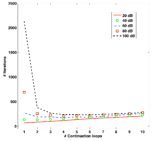
Figure 2: Total number of iterations required for convergence with a varying number of continuation steps and for different values of the dynamic range.

When the ratio $\mu_{0}/\mu_{f}$ is low or when the required accuracy is low, continuation is not as beneficial: intermediate continuation steps require a number of iterations which may not speed up overall convergence. The stepsize which is about $L^{-1}_{\mu_{f}}$ works well in this regime. When the dynamic range increases and we require more accuracy, however, the ratio $\mu_{0}/\mu_{f}$ is large, since $\mu_{0}=.9\|A^{*}b\|_{\ell_{\infty}}\approx\|x\|_{\ell_{\infty}}\gg\sigma$, and continuation provides considerable improvements. In this case, the step size $L^{-1}_{\mu_{f}}$ is too conservative and it takes a while to find the large entries of $x$. Empirically, when the dynamic range is $100$ dB, continuation improves the speed of convergence by a factor of $8$. As this factor is likely to increase exponentially with the dynamic range (when expressed in dB), NESTA with continuation seems to be a better candidate for solving sparse reconstruction problems with high accuracy.

Interestingly, the behavior of NESTA with continuation seems to be quite stable: increasing the number of continuation steps does not increase dramatically the number of iterations. In practice, although the ideal $T$ is certainly signal dependent, we have observed that choosing $T\in\{4,5,6\}$ leads to reasonable results.

3.7 Some theoretical considerations

The convergence of NESTA with and without continuation is straightforward. The following theorem states that each continuation step with $\mu=\mu^{(t)}$ converges to $x^{\star}_{\mu}$. Global convergence is proved by applying this theorem to $t=T$.

Theorem 1.

At each continuation step $t$, $\lim_{k\rightarrow\infty}y_{k}=x_{\mu^{(t)}}^{\star}$, and

$$f_{\mu^{(t)}}(y_{k})-f_{\mu^{(t)}}(x_{\mu^{(t)}}^{\star})\leq\frac{2L_{\mu^{(t)}}\|x_{\mu^{(t)}}^{\star}-x_{\mu^{(t-1)}}\|_{\ell_{2}}^{2}}{k^{2}}.$$

Proof.

Immediate by using [43, Theorem 2]. ∎

As mentioned earlier, continuation may be valuable for improving the speed of convergence. Let each continuation step $t$ stop after $\mathcal{N}^{(t)}$ iterations with

$$\mathcal{N}^{(t)}=\sqrt{\frac{2L_{\mu^{(t)}}}{\gamma^{t}\delta_{0}}}\|x_{\mu^{(t)}}^{\star}-x_{\mu^{(t-1)}}^{\star}\|_{\ell_{2}}$$

so that we have

$$f_{\mu^{(t)}}(y_{k})-f_{\mu^{(t)}}(x_{\mu^{(t)}}^{\star})\leq\gamma^{t}\delta_{0},$$

where the accuracy $\gamma^{t}\delta_{0}$ becomes tighter as $t$ increases. Then summing up the contribution of all the continuation steps gives

$$\mathcal{N}_{c}=\sqrt{\frac{2}{\mu_{0}\delta_{0}}}\sum_{t=1}^{T}\gamma^{-t}\|x_{\mu^{(t)}}^{\star}-x_{\mu^{(t-1)}}^{\star}\|_{\ell_{2}}.$$

When NESTA is applied without continuation, the number of iterations required to reach convergence is

$$\mathcal{N}=\sqrt{\frac{2}{\mu_{0}\delta_{0}}}\gamma^{-T}\|x_{\mu_{f}}^{\star}-x_{0}\|_{\ell_{2}}.$$

Now the ratio $\mathcal{N}_{c}/\mathcal{N}$ is given by

$$\frac{\mathcal{N}_{c}}{\mathcal{N}}=\sum_{t=1}^{T}\gamma^{T-t}\frac{\|x_{\mu^{(t)}}^{\star}-x_{\mu^{(t-1)}}^{\star}\|_{\ell_{2}}}{\|x_{\mu_{f}}^{\star}-x_{0}\|_{\ell_{2}}}.$$ (27)

Continuation is definitely worthwhile when the right-hand side is smaller than $1$. Interestingly, this quantity is directly linked to the path followed by the sequence $x_{0}\rightarrow x_{\mu^{(1)}}\rightarrow\cdots\rightarrow x_{\mu_{f}}$. More precisely, it is related to the smoothness of this path; for instance, if all the intermediate points $x_{\mu^{(t)}}$ belong to the segment $[x_{0},x_{\mu_{f}}]$ in an ordered fashion, then $\sum_{t}\|x_{\mu^{(t)}}^{\star}-x_{\mu^{(t-1)}}\|_{\ell_{2}}=\|x_{\mu_{f}}^{\star}-x_{0}\|_{\ell_{2}}$. Hence, $\frac{\mathcal{N}_{c}}{\mathcal{N}}<1$ and continuation improves the convergence rate.

Figure 3 illustrates two typical solution paths with continuation. When the sequence of solutions obeys $\|x_{0}\|_{\ell_{1}}\geq\ldots\|x_{\mu^{(t)}}^{\star}\|_{\ell_{1}}\ldots\geq\|x_{\mu_{f}}^{\star}\|_{\ell_{1}}$ (this is the case when $x_{0}=A^{*}b$ and $\mu_{1}\geq\ldots\mu^{(t)}\ldots\geq\mu_{f}$), the solution path is likely to be “smooth;” that is, the solutions obey $\|x_{\mu^{(t)}}^{\star}-x_{\mu_{f}}^{\star}\|_{\ell_{2}}\geq\|x_{\mu^{(t+1)}}^{\star}-x_{\mu_{f}}^{\star}\|_{\ell_{2}}$ as on the left of Figure 3. The “nonsmooth” case on the right of Figure 3 arises when the sequence of smoothing parameters does not provide estimates of $x_{\mu_{f}}^{\star}$ that are all better than $x_{0}$. Here, computing some of the intermediate points $\{x_{\mu^{(t)}}^{\star}\}$ is wasteful and continuation fails to be faster.

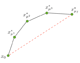
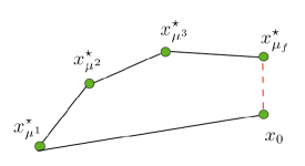
Figure 3: Typical solution paths - Left: smooth solution path. Right: nonsmooth solution path.

4 Accurate Optimization

A significant fraction of the numerical part of this paper focuses on comparing different sparse recovery algorithms in terms of speed and accuracy. In this section, we first demonstrate that NESTA can easily recover the exact solution to $(\text{BP}_{\epsilon})$ with a precision of 5 to 6 digits. Speaking of precision, we shall essentially use two criteria to evaluate accuracy.

1. The first is the (relative) error on the objective functional

   $$\frac{\|x\|_{\ell_{1}}-\|x^{\star}\|_{\ell_{1}}}{\|x^{\star}\|_{\ell_{1}}},$$ (28)

   where $x^{\star}$ is the optimal solution to $(\text{BP}_{\epsilon})$ .

2. The second is the accuracy of the optimal solution itself and is measured via

   $$\|x-x^{\star}\|_{\ell_{\infty}},$$ (29)

   which gives a precise value of the accuracy per entry.

4.1 Is NESTA accurate?

For general problem instances, the exact solution to $(\text{BP}_{\epsilon})$ (or equivalently $(\text{QP}_{\lambda})$) cannot be computed analytically. Under some conditions, however, a simple formula is available when the optimal solution has exactly the same support and the same sign as the unknown (sparse) $x^{0}$ (recall the model $b=Ax^{0}+z$). Denote by $I$ the support of $x^{0}$, $I:=\{i:|x^{0}[i]|>0\}$. Then if $x^{0}$ is sufficiently sparse and if the nonzero entries of $x^{0}$ are sufficiently large, the solution $x^{\star}$ to $(\text{QP}_{\lambda})$ is given by

$$x^{\star}[I] =(A[I]^{*}A[I])^{-1}(A[I]^{*}b-\lambda\,\text{sgn}(x^{0}[I])),$$ (30)

$$x^{\star}[{I^{c}}] =0,$$ (31)

see [12] for example. In this expression, $x[I]$ is the vector with indices in $I$ and $A[I]$ is the submatrix with columns indices in $I$.

To evaluate NESTA’s accuracy, we set $n=262,\!144$, $m=n/8$, and $s=m/100$ (this is the number of nonzero coordinates of $x_{0}$). The absolute values of the nonzero entries of $x_{0}$ are distributed between $1$ and $10^{5}$ so that we have about $100$ dB of dynamic range. The measurements $Ax^{0}$ are discrete cosine coefficients selected uniformly at random. We add Gaussian white noise with standard deviation $\sigma=0.01$. We then compute the solution (30), and make sure it obeys the KKT optimality conditions for $(\text{QP}_{\lambda})$ so that the optimal solution is known.

Table 1: Assessing FISTA’s and NESTA’s accuracy when the optimal solution is known. The relative error on the optimal value is given by (28) and the $\ell_{\infty}$ error on the optimal solution by (29). $\mathcal{N}_{A}$ is the number of calls to $A$ or $A^{*}$ to compute the solution.

Method	$\ell_{1}$-norm	Rel. error $\ell_{1}$-norm	$\ell_{\infty}$ error	$\mathcal{N}_{A}$
$x^{\star}$	3.33601e+6
FISTA	3.33610e+6	2.7e-5	0.31	40000
NESTA $\mu=0.02$	3.33647e+6	1.4e-4	0.08	513

We run NESTA with continuation with the value of $\epsilon:=\|b-Ax^{\star}\|$. We use $\mu=0.02$, $\delta=10^{-7}$ and the number of continuation steps is set to $5$. Table 1 reports on numerical results. First, the value of the objective functional is accurate up to $4$ digits. Second, the computed solution is very accurate since we observe an $\ell_{\infty}$ error of $0.08$. Now recall that the nonzero components of $x^{\star}$ vary from about $1$ to $10^{5}$ so that we have high accuracy over a huge dynamic range. This can also be gleaned from Figure 4 which plots NESTA’s solution versus the optimal solution, and confirms the excellent precision of our algorithm.

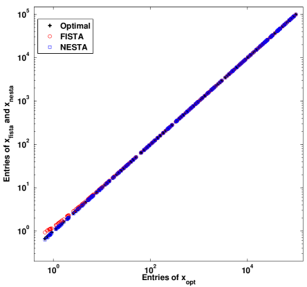
Figure 4: Entries of the computed solutions versus the optimal solution. The absolute values of the entries on the support of the optimal solution are plotted.

4.2 Setting up a reference algorithm for accuracy tests

In general situations, a formula for the optimal solution is of course unavailable, and evaluating the accuracy of solutions requires defining a method of reference. In this paper, we will use FISTA [3] as such a reference since it is an efficient algorithm that also turns out to be extremely easy to use; in particular, no parameter has to be tweaked, except for the standard stopping criterion (maximum number of iterations and tolerance on the relative variation of the objective function).

We run FISTA with $20,\!000$ iterations on the same problem as above, and report its accuracy in Table 1. The $\ell_{1}$-norm is exact up to $4$ digits. Furthermore, Figure 4 shows the entries of FISTA’s solution versus those of the optimal solution, and one observes a very good fit (near perfect when the magnitude of a component of $x^{\star}$ is higher than $3$). The $\ell_{\infty}$ error between FISTA’s solution and the optimal solution $x^{\star}$ is equal to $0.31$; that is, the entries are exact up to $\pm 0.31$. Because this occurs over an enormous dynamic range, we conclude that FISTA also gives very accurate solutions provided that sufficiently many iterations are taken. We have observed that running FISTA with a high number of iterations—typically greater than $20,\!000$—provides accurate solutions to $(\text{QP}_{\lambda})$, and this is why we will use it as our method of reference in the forthcoming comparisons from this section and the next.

4.3 The smoothing parameter $\mu$ and NESTA’s accuracy

By definition, $\mu$ fixes the accuracy of the approximation $f_{\mu}$ to the $\ell_{1}$ norm and, therefore, NESTA’s accuracy directly depends on this parameter. We now propose to assess the accuracy of NESTA for different values of $\mu$. The problem sizes are as before, namely, $n=262,\!144$ and $m=n/8$, except that now the unknown $x^{0}$ is far less sparse with $s=m/5$. The standard deviation of the additive Gaussian white noise is also higher, and we set $\sigma=0.1$.

Because of the larger value of $s$ and $\sigma$, it is no longer possible to have an analytic solution from (30). Instead, we use FISTA to compute a reference solution $x_{F}$, using $20,\!000$ iterations and with $\lambda=0.0685$, which gives $\|b-Ax_{F}\|^{2}_{\ell_{2}}\simeq(m+2\sqrt{2m})\sigma^{2}$. To be sure that FISTA’s solution is very close to the optimal solution, we check that the KKT stationarity condition is nearly verified. If $I_{\star}$ is the support of the optimal solution $x^{\star}$, this condition reads

$$A[I_{\star}]^{*}(b-Ax^{\star}) =\lambda\,\text{sgn}(x^{\star}[I_{\star}]),$$

$$\|A[I_{\star}^{c}]^{*}(b-Ax^{\star})\|_{\ell_{\infty}} \leq\lambda.$$

Now define $I$ to be the support of $x_{F}$. Then, here, $x_{F}$ obeys

$$\|A[I]^{*}(b-Ax_{F})-\lambda\,\text{sgn}(x_{F}[I])\|_{\ell_{\infty}} =2.6610^{-10}\lambda,$$

$$\|A[I^{c}]^{*}(b-Ax_{F})\|_{\ell_{\infty}} \leq 0.99\lambda.$$

This shows that $x_{F}$ is extremely close to the optimal solution.

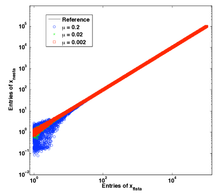
Figure 5: Entries of the computed solutions versus the optimal solution. We plot the absolute values of the entries on the set where the magnitude of the optimal solution exceeds 1.

NESTA is run with $T=5$ continuation steps for three different values of $\mu\in\{0.2,0.02,0.002\}$ (the tolerance $\delta$ is set to $10^{-6}$, $10^{-7}$ and $10^{-8}$ respectively). Figure 5 plots the solutions given by NESTA versus the “optimal solution” $x_{F}$. Clearly, when $\mu$ decreases, the accuracy of NESTA increases just as expected. More precisely, notice in Table 2 that for this particular experiment, decreasing $\mu$ by a factor of $10$ gives about $1$ additional digit of accuracy on the optimal value.

Table 2: NESTA’s accuracy. The errors and number of function calls $\mathcal{N}_{A}$ have the same meaning as in Table 1.

Method	$\ell_{1}$-norm	Rel. error $\ell_{1}$-norm	$\ell_{\infty}$ error	$\mathcal{N}_{A}$
FISTA	5.71539e+7
NESTA $\mu=0.2$	5.71614e+7	1.3e-4	3.8	659
NESTA $\mu=0.02$	5.71547e+7	1.4e-5	0.96	1055
NESTA $\mu=0.002$	5.71540e+7	1.6e-6	0.64	1537

According to this table, $\mu=0.02$ seems a reasonable choice to guarantee an accurate solution since one has between $4$ and $5$ digits of accuracy on the optimal value, and since the $\ell_{\infty}$ error is lower than $1$. Observe that this value separates the nonzero entries from the noise floor (when $\sigma=0.01$). In the extensive numerical experiments of Section 5, we shall set $\mu=0.02$ and $\delta=10^{-7}$ as default values.

5 Numerical comparisons

This section presents numerical experiments comparing several state-of-the-art optimization techniques designed to solve (2) or (3). To be as fair as possible, we propose comparisons with methods for which software is publicly available online. To the best of our knowledge, such extensive comparisons are currently unavailable. Moreover, whereas publications sometimes test algorithms on relatively easy and academic problems, we will subject optimization methods to hard but realistic $\ell_{1}$ reconstruction problems.

In our view, a challenging problem involves some or all of the characteristics below.

1. High dynamic range. As mentioned earlier, most optimization techniques are able to find (more or less rapidly) the most significant entries (those with a large amplitude) of the signal $x$. Recovering the entries of $x$ that have low magnitudes accurately is more challenging.

2. Approximate sparsity. Realistic signals are seldom exactly sparse and, therefore, coping with approximately sparse signals is of paramount importance. In signal or image processing for example, wavelet coefficients of natural images contain lots of low level entries that are worth retrieving.

3. Large scale. Some standard optimization techniques, such as interior point methods, are known to provide accurate solutions. However, these techniques are not applicable to large-scale problems due to the large cost of solving linear systems. Further, many existing software packages fail to take advantage of fast-algorithms for applying $A$. We will focus on large-scale problems in which the number of unknowns $n$ is over a quarter of a million, i.e. $n=262,\!144$.

5.1 State-of-the-art methods

Most of the algorithms discussed in this section are considered to be state-of-art in the sense that they are the most competitive among sparse reconstruction algorithms. To repeat ourselves, many of these methods have been improved after several years of research [36, 31], and many did not exist two years ago [34, 51]. For instance, [35] was submitted for publication less than three months before we put the final touches on this paper. Finally, our focus is on rapid algorithms so that we are interested in methods which can take advantage of fast algorithms for applying $A$ to a vector. This is why we have not tested other good methods such as [32], for example.

5.1.1 NESTA

Below, we applied NESTA with the following default parameters

$$x_{0}=A^{*}b,\quad\mu=0.02,\quad\delta=10^{-7}$$

(recall that $x_{0}$ is the initial guess). The maximal number of iterations is set to $\mathcal{I}_{\max}=10,\!000$; if convergence is not reached after $\mathcal{I}_{\max}$ iterations, we record that the algorithm did not convergence (DNC). Because NESTA requires 2 calls to either $A$ or $A^{*}$ per iteration, this is equivalent to declaring DNC after $\mathcal{N}_{A}=20,\!000$ iterations where $\mathcal{N}_{A}$ refers to the total number of calls to $A$ or $A^{*}$; hence, for the other methods, we declare DNC when $\mathcal{N}_{A}>20,\!000$. When continuation is used, extra parameters are set up as follows:

$$T=4,\quad\mu_{0}=\|x_{0}\|_{\ell_{\infty}},\quad\gamma=(\mu/\mu_{0})^{1/T},$$

and for $t=1,\ldots,T$,

$$\mu_{t}=\gamma^{t}\mu_{0},\quad\delta_{t}=0.1\cdot(\delta/0.1)^{t/T}.$$

Numerical results are reported and discussed in Section 5.4.

5.1.2 Gradient Projections for Sparse Reconstruction (GPSR) [31]

GPSR has been introduced in [31] to solve the standard $\ell_{1}$ minimization problem in Lagrangian form ($\text{QP}_{\lambda}$). GPSR is based on the well-known projected gradient step technique,

$$v^{(k+1)}=\mathcal{P}_{\mathcal{Q}}\left(v^{(k-1)}-\alpha_{k}\nabla F(v_{k})\right),$$

for some projector $\mathcal{P}_{\mathcal{Q}}$ onto a convex set $\mathcal{Q}$; this set contains the variable of interest $v$. In this equation, $F$ is the function to be minimized. In GPSR, the problem is recast such that the variable $v=[v_{1},v_{2}]$ has positive entries and $x=v_{1}-v_{2}$ (a standard change of variables in linear programming methods). The function $F$ is then

$$F(v)=\lambda\,\underline{1}^{*}v+\frac{1}{2}\|b-[A,-A]v\|_{\ell_{2}}^{2},$$

where $\underline{1}$ is the vector of ones, and $v$ belongs to the nonnegative orthant, $v[i]\geq 0$ for all $i$. The projection onto $\mathcal{Q}$ is then trivial. Different techniques for choosing the step-size $\alpha_{k}$ (backtracking, Barzilai-Borwein [2], and so on) are discussed in [31]. The code is available at http://www.lx.it.pt/~mtf/GPSR/. In the forthcoming experiments, the parameters are set to their default values.

GPSR also implements continuation, and we test this version as well. All parameters were set to defaults except, per the recommendation of one of the GPSR authors to increase performance, the number of continuation steps was set to 40, the ToleranceA variable was set to $10^{-3}$, and the MiniterA variable was set to $1$. In addition, the code itself was tweaked a bit; in particular, the stopping criteria for continuation steps (other than the final step) was changed. Future releases of GPSR will probably contain a similarly updated continuation stopping criteria.

5.1.3 Sparse reconstruction by separable approximation (SpaRSA) [54]

SpaRSA is an algorithm to minimize composite functions $\phi(x)=f(x)+\lambda c(x)$ composed of a smooth term $f$ and a separable non-smooth term $c$, e.g. ($\text{QP}_{\lambda}$). At every step, a subproblem of the form

$$\text{minimize}\quad\|x-y\|_{\ell_{2}}^{2}+\frac{\lambda}{\alpha}c(x)$$

with optimization variable $x$ must be solved; this is the same as computing the proximity operator corresponding to $c$. For ($\text{QP}_{\lambda}$), the solution is given by shrinkage. In this sense, SpaRSA is an iterative shrinkage/thresholding (IST) algorithm, much like FISTA (though without the accelerated convergence) and FPC. Also like FPC, continuation is used to speed convergence, and like FPC-BB, a Barzilai-Borwein heuristic is used for the step size $\alpha$ (instead of using a pessimistic bound like the Lipschitz constant). With this choice, SpaRSA is not guaranteed to be monotone, which can be remedied by implementing an appropriate safeguard, although this is not done in practice because there is little experimental advantage to doing so. Code for SpaRSA may be obtained at http://www.lx.it.pt/~mtf/SpaRSA/. Parameters were set to default except the number of continuation steps was set to 40 and the MiniterA variable was set to 1 (instead of the default 5), as per the recommendations of one of the SpaRSA authors—again, as to increase performance.

5.1.4 $\ell_{1}$ regularized least squares (l1_ls) [36]

This method solves the standard unconstrained $\ell_{1}$ minimization problem, and is an interior point method (with log-barrier) using preconditioned conjugate gradient (PCG) to accelerate convergence and stabilize the algorithm. The preconditioner used in the PCG step is a linear combination of the diagonal approximation of the Hessian of the quadratic term and of the Hessian of the log-barrier term. l1_ls is shown to be faster than usual interior point methods; nevertheless, each step requires solving a linear system of the form $H\Delta x=g$. Even if PCG makes the method more reliable, l1_ls is still problematic for large-scale problems. In the next comparisons, we provide some typical values of its computational complexity compared to the other methods. The code is available at http://www.stanford.edu/~boyd/l1_ls/.

5.1.5 Spectral projected gradient (SPGL1) [51]

In 2008, van den Berg et al. adapted the spectral projection gradient algorithm introduced in [6] to solve the LASSO ($\text{LS}_{\tau}$). Interestingly, they introduced a clever root finding procedure such that solving a few instances of $(\text{LS}_{\tau})$ for different values of $\tau$ enables them to equivalently solve ($\text{BP}_{\epsilon}$). Furthermore, if the algorithm detects a nearly-sparse solution, it defines an active set and solves an equation like (30) on this active set. In the next experiments, the parameters are set to their default values. The code is available at http://www.cs.ubc.ca/labs/scl/SPGL11/.

5.1.6 Fixed Point Continuation method (FPC) [34, 35]

The Fixed Point Continuation method is a recent first-order algorithm for solving $(\text{QP}_{\lambda})$ and simple generalizations of $(\text{QP}_{\lambda})$ ​. The main idea is based on a fixed point equation, $x=F(x)$, which holds at the solution (derived from the subgradient optimality condition). For appropriate parameters, $F$ is a contraction, and thus the algorithm $x_{k+1}=F(x_{k})$ converges. The operator $F$ comes from forward-backward splitting, and consists of a soft-thresholding/shrinkage step and a gradient step. The main computational burden is one application of $A$ and $A^{*}$ at every step. The papers [34, 35] prove $q$-linear convergence, and finite-convergence of some of the components of $x$ for $s$-sparse signals. The parameter $\lambda$ in $(\text{QP}_{\lambda})$ determines the amount of shrinkage and, therefore, the speed of convergence; thus in practice, $\lambda$ is decreased in a continuation scheme. Code for FPC is available at http://www.caam.rice.edu/~optimization/L1/fpc/. Also available is a state-of-the-art version of FPC from 2008 that uses Barzilai-Borwein [2] steps to accelerate performance. In the numerical tests, the Barzilai-Borwein version (referred to as FPC-BB) significantly outperforms standard FPC. All parameters were set to default values.

5.1.7 FPC Active Set (FPC-AS) [53]

In 2009, inspired by both first-order algorithms, such as FPC, and greedy algorithms [28, 40], Wen et al. [53] extend FPC into the two-part algorithm FPC Active Set to solve $(\text{QP}_{\lambda})$ ​​. In the first stage, FPC-AS calls an improved version of FPC that allows the step-size to be updated dynamically, using a non-monotone exact line search to ensure $r$-linear convergence, and a Barzilai-Borwein [2] heuristic. After a given stopping criterion, the current value, $x_{k}$, is hard-thresholded to determine an active set. On the active set, $\|x\|_{\ell_{1}}$ is replaced by $c^{*}x$, where $c=\text{sgn}(x_{k})$, with the constraints that $x[i]\cdot c[i]>0$ for all the indices $i$ belonging to the active set. The objective is now smooth, and solvers, like conjugate gradients (CG) or quasi-Newton methods (e.g. L-BFGS or L-BFGS-B), can solve for $x$ on the active set; this the same as solving (30). This two-step process is then repeated for a smaller value of $\lambda$ in a continuation scheme. We tested FPC-AS using both L-BFGS (the default) and CG (which we refer to as FPC-AS-CG) to solve the subproblem; both of these solvers do not actually enforce the $x[i]\cdot c[i]>0$ constraint on the active set. Code for FPC-AS is available at http://www.caam.rice.edu/~optimization/L1/FPC_AS/.

For $s$-sparse signals, all parameters were set to defaults except for the stopping criteria (as discussed in Section 5.3). For approximately sparse signals, FPC-AS performed poorly ($>10,000$ iterations) with the default parameters. By changing a parameter that controls the estimated number of nonzeros from $m/2$ (default) to $n$, the performance improved dramatically, and this is the performance reported in the tables. The maximum number of subspace iterations was also changed from the default to 10, as recommended in the help file.

5.1.8 Bregman

The Bregman Iterative algorithm, motivated by the Bregman distance, has been shown to be surprisingly simple [56]. The first iteration solves $(\text{QP}_{\lambda})$ for a specified value of $\lambda$; subsequent iterations solve $(\text{QP}_{\lambda})$ for the same value of $\lambda$, with an updated observation vector $b$. Typically, only a few outer iterations are needed (e.g. 4), but each iteration requires a solve of ($\text{QP}_{\lambda}$), which is costly. The original Bregman algorithm calls FPC to solve these subproblems; we test Bregman using FPC and the Barzilai-Borwein version of FPC as subproblem solvers.

A version of the Bregman algorithm, known as the Linearized Bregman algorithm [46, 9], takes only one step of the inner iteration per outer iteration; consequently, many outer iterations are taken, in contrast to the regular Bregman algorithm. It can be shown that linearized Bregman is equivalent to gradient ascent on the dual problem. Linearized Bregman was not included in the tests because no standardized public code is available. Code for the regular Bregman algorithm may be obtained at http://www.caam.rice.edu/~optimization/L1/2006/10/bregman-iterative-algorithms-for.html. There are quite a few parameters, since there are parameters for the outer iterations and for the inner (FPC) iterations; for all experiments, parameters were set to defaults. In particular, we noted that using the default stopping criteria for the inner solve, which limited FPC to $1,\!000$ iterations, led to significantly better results than allowing the subproblem to run to $10,\!000$ iterations.

5.1.9 Fast Iterative Soft-Thresholding Algorithm (FISTA)

FISTA is based upon Nesterov’s work but departs from NESTA in two important ways: 1) FISTA solves the sparse unconstrained reconstruction problem ($\text{QP}_{\lambda}$); 2) FISTA is a proximal subgradient algorithm, which only uses two sequences of iterates. In some sense, FISTA is a simplified version of the algorithm previously introduced by Nesterov to minimize composite functions [44]. The theoretical rate of convergence of FISTA is similar to NESTA’s, and has been shown to decay as $\mathcal{O}(1/k^{2})$.

For each test, FISTA is run twice: it is first run until the relative variation in the function value is less than $10^{-14}$, with no limit on function calls, and this solution is used as the reference solution. It is then run a second time using either Criteria 1 or Criteria 2 as the stopping condition, and these are the results reported in the tables.

5.2 Constrained versus unconstrained minimization

We would like to briefly highlight the fact that these algorithms are not solving the same problem. NESTA and SPGL1 solve the constrained problem ($\text{BP}_{\epsilon}$), while all other methods tested solve the unconstrained problem ($\text{QP}_{\lambda}$). As the first chapter of any optimization book will emphasize, solving an unconstrained problem is in general much easier than a constrained problem. For example, it may be hard to even find a feasible point for ($\text{BP}_{\epsilon}$), since the pseudo-inverse of $A$, when $A$ is not a projection, may be difficult to compute. It is possible to solve a sequence of unconstrained ($\text{QP}_{\lambda_{j}}$) problems for various $\lambda_{j}$ to approximately find a value of the dual variable $\lambda$ that leads to equivalence with ($\text{BP}_{\epsilon}$), but even if this procedure is integrated with the continuation procedure, it will require several, if not dozens, of solves of $(\text{QP}_{\lambda})$ (and this will in general only lead to an approximate solution to ($\text{BP}_{\epsilon}$)). The Newton-based root finding method of SPGL1 relies on solving a sequence of constrained problems ($\text{LS}_{\tau}$); basically, the dual solution to a constrained problem gives useful information.

Thus, we emphasize that SPGL1 and NESTA are actually more general than the other algorithms (and as Section 6 shows, NESTA is even more general because it handles a wide variety of constrained problems); this is especially important because from a practical viewpoint, it may be easier to estimate an appropriate $\epsilon$ than an appropriate value of $\lambda$. Furthermore, as will be shown in Section 5.4, SPGL1 and NESTA with continuation are also the most robust methods for arbitrary signals (i.e. they perform well even when the signal is not exactly sparse, and even when it has high dynamic range). Combining these two facts, we feel that these two algorithms are extremely useful for real-world applications.

5.3 Experimental protocol

In these experiments, we compare NESTA with other efficient methods. There are two main difficulties with comparisons which might explain why broad comparisons have not been offered before. The first problem is that some algorithms, such as NESTA, solve ($\text{BP}_{\epsilon}$), whereas other algorithms solve ($\text{QP}_{\lambda}$). Given $\epsilon$, it is difficult to compute $\lambda(\epsilon)$ that gives an equivalence between the problems; in theory, the KKT conditions give $\lambda$, but we have observed in practice that because we have an approximate solution (albeit a very accurate one), computing $\lambda$ in this fashion is not stable.

Instead, we note that given $\lambda$ and a solution $x_{\lambda}$ to ($\text{QP}_{\lambda}$), it is easy to compute a very accurate $\epsilon(\lambda)$ since $\epsilon=\|Ax_{\lambda}-b\|_{\ell_{2}}$. Hence, we use a two-step procedure. In the first step, we choose a value of $\epsilon_{0}=\sqrt{m+2\sqrt{2m}}\sigma$ based on the noise level $\sigma$ (since a value of $\lambda$ that corresponds to $\sigma$ is less clear), and use SPGL1 to solve ($\text{BP}_{\epsilon}$). From the SPGL1 dual solution, we have an estimate of $\lambda=\lambda(\epsilon_{0})$. As noted above, this equivalence may not be very accurate, so the second step is to compute $\epsilon_{1}=\epsilon(\lambda)$ via FISTA, using a very high accuracy of $\delta=10^{-14}$. The pair $(\lambda,\epsilon_{1})$ now leads to nearly equivalent solutions of ($\text{QP}_{\lambda}$) and ($\text{BP}_{\epsilon}$). The solution from FISTA will also be used to judge the accuracy of the other algorithms.

The other main difficulty in comparisons is a fair stopping criterion. Each algorithm has its own stopping criterion (or may offer a choice of stopping criteria), and these are not directly comparable. To overcome this difficulty, we have modified the codes of the algorithms to allow for two new stopping criterion that we feel are the only fair choices. The short story is that we use NESTA to compute a solution $x_{N}$ and then ask the other algorithms to compute a solution that is at least as accurate.

Specifically, given NESTA’s solution $x_{N}$ (using continuation), the other algorithms terminate at iteration $k$ when the solution $\hat{x}_{k}$ satisfies

$$\text{(Crit.\leavevmode\nobreak\ 1)}\quad\|\hat{x}_{k}\|_{\ell_{1}}\leq\|x_{N}\|_{\ell_{1}}\quad\text{and}\quad\|b-A\hat{x}_{k}\|_{\ell_{2}}\leq 1.05\,\|b-Ax_{N}\|_{\ell_{2}},$$ (32)

or

$$\text{(Crit.\leavevmode\nobreak\ 2)}\quad\lambda\|\hat{x}_{k}\|_{\ell_{1}}+\frac{1}{2}\|A\hat{x}_{k}-b\|_{\ell_{2}}^{2}\leq\lambda\|x_{N}\|_{\ell_{1}}+\frac{1}{2}\|Ax_{N}-b\|_{\ell_{2}}^{2}.$$ (33)

We run tests with both stopping criteria to reduce any potential bias from the fact that some algorithms solve ($\text{QP}_{\lambda}$), for which Crit. 2 is the most natural, while others solve ($\text{BP}_{\epsilon}$), for which Crit. 1 is the most natural. In practice, the results when applying Crit. 1 or Crit. 2 are not significantly different.

5.4 Numerical results

5.4.1 The case of exactly sparse signals

This first series of experiments tests all the algorithms discussed above in the case where the unknown signal is $s$-sparse with $s=m/5$, $m=n/8$, and $n=262,\!144$. This situation is close to the limit of perfect recovery from noiseless data. The $s$ nonzero entries of the signals $x^{0}$ are generated as described in (26). Reconstruction is performed with several values of the dynamic range $d=20,40,60,80,100$ in dB. The measurement operator is a randomly subsampled discrete cosine transform, as in Section 4.1 (with a different random set of measurements chosen for each trial). The noise level is set to $\sigma=0.1$. The results are reported in Tables 3 (Crit. 1) and 4 (Crit. 2); each cell in these table contains the mean value of $\mathcal{N}_{A}$ (the number of calls of $A$ or $A^{*}$) over $10$ random trials, and, in smaller font, the minimum and maximum value of $\mathcal{N}_{A}$ over the $10$ trials. When convergence is not reached after $\mathcal{N}_{A}=20,\!000$, we report DNC (did not converge). As expected, the number of calls needed to reach convergence varies a lot from an algorithm to another.

Table 3: Number of function calls $\mathcal{N}_{A}$ averaged over 10 independent runs. The sparsity level $s=m/5$ and the stopping rule is Crit. 1 (32).

Method	20 dB	40 dB	60 dB	80 dB	100 dB
NESTA	446 351/491	880 719/951	1701 1581/1777	4528 4031/4749	14647 7729/15991
NESTA + Ct	479 475/485	551 539/559	605 589/619	658 635/679	685 657/705
GPSR	56 44/62	733 680/788	5320 4818/5628	DNC	DNC
GPSR + Ct	305 293/311	251 245/257	497 453/531	1816 1303/2069	9101 7221/10761
SpaRSA	345 327/373	455 435/469	542 511/579	601 563/629	708 667/819
SPGL1	54 37/61	128 102/142	209 190/216	354 297/561	465 380/562
FISTA	68 66/69	270 261/279	935 885/969	3410 2961/3594	13164 11961/13911
FPC AS	156 111/177	236 157/263	218 215/239	351 247/457	325 313/335
FPC AS (CG)	312 212/359	475 301/538	434 423/481	641 470/812	583 567/595
FPC	414 394/436	417 408/422	571 546/594	945 852/1038	3945 2018/4734
FPC-BB	148 140/152	166 158/168	219 208/250	264 252/282	520 320/800
Bregman-BB	211 203/225	270 257/295	364 355/393	470 429/501	572 521/657

Table 4: Number of function calls $\mathcal{N}_{A}$ averaged over 10 independent runs. The sparsity level $s=m/5$ and the stopping rule is Crit. 2 (33).

Method	20 dB	40 dB	60 dB	80 dB	100 dB
NESTA	446 351/491	880 719/951	1701 1581/1777	4528 4031/4749	14647 7729/15991
NESTA + Ct	479 475/485	551 539/559	605 589/619	658 635/679	685 657/705
GPSR	59 44/64	736 678/790	5316 4814/5630	DNC	DNC
GPSR + Ct	305 293/311	251 245/257	511 467/543	1837 1323/2091	9127 7251/10789
SpaRSA	345 327/373	455 435/469	541 509/579	600 561/629	706 667/819
SPGL1	55 37/61	138 113/152	217 196/233	358 300/576	470 383/568
FISTA	65 63/66	288 279/297	932 882/966	3407 2961/3591	13160 11955/13908
FPC AS	176 169/183	236 157/263	218 215/239	344 247/459	330 319/339
FPC AS (CG)	357 343/371	475 301/538	434 423/481	622 435/814	588 573/599
FPC	416 398/438	435 418/446	577 558/600	899 788/962	3866 1938/4648
FPC-BB	149 140/154	172 164/174	217 208/254	262 248/286	512 308/790
Bregman-BB	211 203/225	270 257/295	364 355/393	470 429/501	572 521/657

The careful reader will notice that Tables 3 and 4 do not feature the results provided by l1_ls; indeed, while it seems faster than other interior point methods, it is still far from being comparable to the other algorithms reviewed here. In these experiments l1_ls typically needed $1500$ calls to $A$ or $A^{*}$ for reconstructing a $20$ dB signal with $s=m/100$ nonzero entries. For solving the same problem with a dynamic range of $100$ dB, it took $\leavevmode\nobreak\ 5$ hours to converge on a dual core MacPro G5 clocked at 2.7GHz.

GPSR performs well in the case of low-dynamic range signals; its performance, however, decreases dramatically as the dynamic range increases; Table 4 shows that it does not converge for 80 and 100 dB signals. GPSR with continuation does worse on the low dynamic range signals (which is not surprising). It does much better than the regular GPSR version on the high dynamic range signals, though it is slower than NESTA with continuation by more than a factor of 10. SpaRSA performs well at low dynamic range, comparable to NESTA, and begins to outperform GSPR with continuation as the dynamic range increases, although it begins to underperform NESTA with continuation in this regime. SpaRSA takes over twice as many function calls on the 100 dB signal as on the 20 dB signal.

SPGL1 shows good performance with very sparse signals and low dynamic range. Although it has fewer iteration counts than NESTA, the performance decreases much more quickly than for NESTA as the dynamic range increases; SPGL1 requires about 9$\times$ more calls to $A$ at 100 dB than at 20 dB, whereas NESTA with continuation requires only about 1.5$\times$ more calls. FISTA is almost as fast as SPGL1 on the low dynamic range signal, but degrades very quickly as the dynamic range increases, taking about 200$\times$ more iterations at 100 dB than at 20 dB. One large contributing factor to this poor performance at high dynamic range is the lack of a continuation scheme.

FPC performs well at low dynamic range, but is very slow on 100 dB signals. The Barzilai-Borwein version was consistently faster than the regular version, but also degrades much faster than NESTA with continuation as the dynamic range increases. Both FPC Active Set and the Bregman algorithm perform well at all dynamic ranges, but again, degrade faster than NESTA with continuation as the dynamic range increases. There is a slight difference between the two FPC Active set versions (using L-BFGS or CG), but the dependence on the dynamic range is roughly similar.

The performances of NESTA with continuation are reasonable when the dynamic range is low. When the dynamic range increases, continuation helps by dividing the number of calls up to a factor about $20$, as in the 100 dB case. In these experiments, the tolerance $\delta$ is consistently equal to $10^{-7}$; while this choice is reasonable when the dynamic range is high, it seems too conservative in the low dynamic range case. Setting a lower value of $\delta$ should improve NESTA’s performance in this regime. In other words, NESTA with continuation might be tweaked to run faster on the low dynamic range signals. However, this is not in the spirit of this paper and this is why we have not researched further refinements.

In summary, for exactly sparse signals exhibiting a significant dynamic range, 1) the performance of NESTA with continuation—but otherwise applied out-of-the-box—is comparable to that of state-of-the-art algorithms, and 2) most state-of-the-art algorithms are efficient on these types of signals.

5.4.2 Approximately sparse signals

We now turn our attention to approximately sparse signals. Such signals are generated via a permutation of the Haar wavelet coefficients of a $512\times 512$ natural image. The data $b$ are $m=n/8=32,\!768$ discrete cosine measurements selected at random. White Gaussian noise with standard deviation $\sigma=0.1$ is then added. Each test is repeated 5 times, using a different random permutation every time (as well as a new instance of the noise vector). Unlike in the exactly sparse case, the wavelet coefficients of natural images mostly contain mid-range and low level coefficients (see Figure 6) which are challenging to recover.

Figure 6: Sorted wavelet coefficients of the natural image used in the experiments.

The results are reported in Tables 5 (Crit. 1) and 6 (Crit. 2); the results from applying the two stopping criteria are nearly identical. In these series of experiments, the performance of SPGL1 is quite good but seems to vary a lot from one trial to another (Table 6). Notice that the concept of an active-set is ill defined in the approximately sparse case; as a consequence, the active set version of FPC is not much of an improvement over the regular FPC version. FPC is very fast for $s$-sparse signals but lacks the robustness to deal with less ideal situations in which the unknown is only approximately sparse.

FISTA and SpaRSA converge for these tests, but are not competitive with the best methods. It is reasonable to assume that FISTA would also improve if implemented with continuation. SpaRSA already uses continuation but does not match its excellent performance on exactly sparse signals.

Bregman, SPGL1, and NESTA with continuation all have excellent performances (continuation really helps NESTA) in this series of experiments. NESTA with continuation seems very robust when high accuracy is required. The main distinguishing feature of NESTA is that it is less sensitive to dynamic range; this means that as the dynamic range increases, or as the noise level $\sigma$ decreases, NESTA becomes very competitive. For example, when the same test was repeated with more noise ($\sigma=1$), all the algorithms converged faster. In moving from $\sigma=1$ to $\sigma=0.1$, SPGL1 required $90\%$ more iterations and Bregman required $20\%$ more iterations, while NESTA with continuation required only $5\%$ more iterations.

One conclusion from these tests is that SPGL1, Bregman and NESTA (with continuation) are the only methods dealing with approximately sparse signals effectively. The other methods, most of which did very well on exactly sparse signals, take over $10,\!000$ function calls or even do not converge in $20,\!000$ function calls; by comparison, SPGL1, Bregman and NESTA with continuation converge in about $2,\!000$ function calls. It is also worth noting that Bregman is only as good as the subproblem solver; though not reported here, using the regular FPC (instead of FPC-BB) with Bregman leads to much worse performance.

The algorithms which did converge all achieved a mean relative $\ell_{1}$ error (using (28) and the high accuracy FISTA solution as the reference) less than $2\cdot 10^{-4}$ and sometimes as low as $10^{-5}$, except SPGL1, which had a mean relative error of $1.1\cdot 10^{-3}$. Of the algorithms that did not converge in $20,\!000$ function calls, FPC and FPC-BB had a mean $\ell_{1}$ relative error about $5\cdot 10^{-3}$, GPSR with continuation had errors about $5\cdot 10^{-2}$, and the rest had errors greater than $10^{-1}$.

Table 5: Recovery results of an approximately sparse signal with Crit. $1$ as a stopping rule.

Method	$<\mathcal{N}_{A}>$	$\min\mathcal{N}_{A}$	$\max\mathcal{N}_{A}$
NESTA	18912	18773	19115
NESTA + Ct	2667	2603	2713
GPSR	DNC	DNC	DNC
GPSR + Ct	DNC	DNC	DNC
SpaRSA	10019	8369	12409
SPGL1	1776	1073	2464
FISTA	10765	10239	11019
FPC Active Set	DNC	DNC	DNC
FPC Active Set (CG)	DNC	DNC	DNC
FPC	DNC	DNC	DNC
FPC-BB	DNC	DNC	DNC
Bregman-BB	2045	2045	2045

Table 6: Recovery results of an approximately sparse signal with Crit. $2$ as a stopping rule.

Method	$<\mathcal{N}_{A}>$	$\min\mathcal{N}_{A}$	$\max\mathcal{N}_{A}$
NESTA	18912	18773	19115
NESTA + Ct	2667	2603	2713
GPSR	DNC	DNC	DNC
GPSR + Ct	DNC	DNC	DNC
SpaRSA	10021	8353	12439
SPGL1	1776	1073	2464
FISTA	10724	10197	10980
FPC Active Set	DNC	DNC	DNC
FPC Active Set (CG)	DNC	DNC	DNC
FPC	DNC	DNC	DNC
FPC-BB	DNC	DNC	DNC
Bregman-BB	2045	2045	2045

6 An all-purpose algorithm

A distinguishing feature is that NESTA is able to cope with a wide range of standard regularizing functions. In this section, we present two examples: nonstandard $\ell_{1}$ minimization and total-variation minimization.

6.1 Nonstandard sparse reconstruction: $\ell_{1}$ analysis

Suppose we have a signal $x\in\mathbb{R}^{n}$, which is assumed to be approximately sparse in a transformed domain such as the wavelet, the curvelet or the time-frequency domains. Let $W$ be the corresponding synthesis operator whose columns are the waveforms we use to synthesize the signal $x=W\alpha$ (real-world signals do not admit an exactly sparse expansion); e.g. the columns may be wavelets, curvelets and so on, or both. We will refer to $W^{*}$ as the analysis operator. As before, we have (possibly noisy) measurements $b=Ax^{0}+z$. The synthesis approach attempts reconstruction by solving

$$\begin{array}[]{ll}\text{minimize}&\quad\|\alpha\|_{\ell_{1}}\\ \text{subject to}&\quad\|b-AW\alpha\|_{\ell_{2}}\leq\epsilon,\end{array}$$ (34)

while the analysis approach solves the related problem

$$\begin{array}[]{ll}\text{minimize}&\quad\|W^{*}x\|_{\ell_{1}}\\ \text{subject to}&\quad\|b-Ax\|_{\ell_{2}}\leq\epsilon.\end{array}$$ (35)

If $W$ is orthonormal, the two problems are equivalent, but in general, these give distinct solutions and current theory explaining the differences is still in its infancy. The article [29] suggests that synthesis may be overly sensitive, and argues with geometric heuristics and numerical simulations that analysis is sometimes preferable.

Solving $\ell_{1}$-analysis problems with NESTA is straightforward as only Step $1$ needs to be adapted. We have

$$f_{\mu}(x)=\max_{x\mathcal{Q}_{s}}\langle u,W^{*}x\rangle-\frac{\mu}{2}\|u\|_{\ell_{2}}^{2},$$

and the gradient at $x$ is equal to

$$\nabla f_{\mu}(x)=Wu_{\mu}(x);$$

here, $u_{\mu}(x)$ is given by

$$(u_{\mu}(x))[i]=\begin{cases}\mu^{-1}(W^{*}x)[i],&\text{if }|(W^{*}x)[i]|<\mu,\\ \text{sgn}((W^{*}x)[i]),&\text{otherwise}.\end{cases}$$

Steps $2$ and $3$ remain unchanged. The computational complexity of the algorithm is then increased by an extra term, namely $2\,\mathcal{C}_{W}$ where $\mathcal{C}_{W}$ is the cost of applying $W$ or $W^{*}$ to a vector. In practical situations, there is often a fast algorithm for applying $W$ and $W^{*}$, e.g. a fast wavelet transform [39], a fast curvelet transform [11], a fast short-time Fourier transform [39] and so on, which makes this a low-cost extra step.

6.2 Numerical results for nonstandard $\ell_{1}$ minimization

Because NESTA is one of very few algorithms that can solve both the analysis and synthesis problems efficiently, we tested the performance of both analysis and synthesis on a simulated real-world signal from the field of radar detection. The test input is a superposition of three signals. The first signal, which is intended to make recovery more difficult for any smaller signals, is a plain sinusoid with amplitude of 1000 and frequency near 835 MHz.

A second signal, similar to a Doppler pulse radar, is at a carrier frequency of 2.33 GHz with maximum amplitude of 10, a pulse width of 1 $\mu s$ and a pulse repetition interval of 10 $\mu$s; the pulse envelope is trapezoidal, with a 10 ns rise time and 40 ns fall time. This signal is more than 40 dB lower than the pure sinusoid, since the maximum amplitude is 100$\times$ smaller, and since the radar is nonzero only 10% of the time. The Doppler pulse was chosen to be roughly similar to a realistic weather Doppler radar. In practice, these systems operate at 5 cm or 10 cm wavelengths (i.e. 6 or 3 GHz) and send out short trapezoidal pulses to measure the radial velocity of water droplets in the atmosphere using the Doppler effect.

The third signal, which is the signal of interest, is a frequency-hopping radar pulse with maximum amplitude of 1 (so about 20 dB beneath the Doppler signal, and more than 60 dB below the sinusoid). For each instance of the pulse, the frequency is chosen uniformly at random from the range 200 MHz to 2.4 GHz. The pulse duration is 2 $\mu s$ and the pulse repetition interval is 22 $\mu s$, which means that some, but not all, pulses overlap with the Doppler radar pulses. The rise time and fall time of the pulse envelope are comparable to the Doppler pulse. Frequency-hopping signals may arise in applications because they can be more robust to interference and because they can be harder to intercept. When the carrier frequencies are not known to the listener, the receiver must be designed to cover the entire range of possible frequencies (2.2 GHz in our case). While some current analog-to-digital converters (ADC) may be capable of operating at 2.2 GHz, they do so at the expense of low precision. Hence this situation may be particularly amenable to a compressed sensing setup by using several slower (but accurate) ADC to cover a large bandwidth.

We consider the exact signal to be the result of an infinite-precision ADC operating at 5 GHz, which corresponds to the Nyquist rate for signals with 2.5 GHz of bandwidth. Measurements are taken using an orthogonal Hadamard transform with randomly permuted columns, and these measurements were subsequently sub-sampled by randomly choosing $m=.3n$ rows of the transform (so that we undersample Nyquist by $10/3$). Samples are recorded for $T=209.7\mu$s, which corresponds to $n=2^{20}$. White noise was added to the measurements to make a 60 dB signal-to-noise ratio (SNR) (note that the effective SNR for the frequency-hopping pulse is much lower). The frequencies of the sinusoid and the Doppler radar were chosen such that they were not integer multiples of the lowest recoverable frequency $f_{min}=1/(2T)$.

For reconstruction, the signal is analyzed with a tight frame of Gabor atoms that is approximately 5.5$\times$ overcomplete. The particular parameters of the frame are chosen to give reasonable reconstruction, but were not tweaked excessively. It is likely that differences in performance between analysis and synthesis are heavily dependent on the particular dictionary.

To analyze performance, we restrict our attention to the frequency domain in order to simplify comparisons. The top plot in Figure 7 shows the frequency components of the original, noiseless signal. The frequency hopping pulse barely shows up since the amplitude is 1000$\times$ smaller than the sinusoid and since each frequency only occurs for 1 $\mu$s (of 210 $\mu$s total).

The bottom plots in Figure 7 show the spectrum of the recovered signal using analysis and synthesis, respectively. For this test, analysis does a better job at finding the frequencies belonging to the small pulse, while synthesis does a better job recreating the large pulse and the pure tone. The two reconstructions used slightly different values of $\mu$ to account for the redundancy in the size of the dictionary; otherwise, algorithm parameters were the same. In the analysis problem, NESTA took 231 calls to the analysis/synthesis operator (and 231 calls to the Hadamard transform); for synthesis, NESTA took 1378 calls to the analysis/synthesis operator (and 1378 to the Hadamard transform). With NESTA, synthesis is more computationally expensive than analysis since no change of variables trick can be done; in the synthesis case, $W$ and $W^{*}$ are used in Step $2$ and $3$ while in the analysis case, the same operators are used once in Step $1$ (this is accomplished by the previously mentioned change-of-variables for partial orthogonal measurements).

As emphasized in [29], when $W$ is overcomplete, the solution computed by solving the analysis problems is likely to be denser than in the synthesis case. In plain English, the analysis solution may seem “noisier” than the synthesis solution. But the compactness of the solution of the synthesis problem may also be its weakness: an error on one entry of $\alpha$ may lead to a solution that differs a lot. This may explain why the frequency-hopping radar pulse is harder to recover with the synthesis prior.

Because all other known first-order methods solve only the synthesis problem, NESTA may prove to be extremely useful for real-world applications. Indeed, this simple test suggests that analysis may sometimes be much preferable to synthesis, and given a signal with $2^{20}$ samples (too large for interior point methods), we know of no other algorithm that can return the same results.

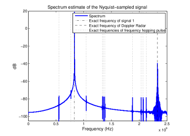
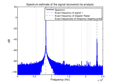
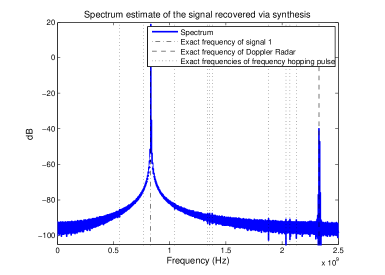
Figure 7: Top: spectrum estimate of the exact signal, no noise. The pure tone at 60 dB and the Doppler radar at 20 dB dominate the 0 dB frequency hopping pulses. Middle: spectrum estimate of the recovered signal using analysis prior, with 60 dB SNR. The spectrum appears noisy, but the frequency hopping pulses stand out. Bottom: spectrum estimate of the recovered signal using synthesis prior, with 60 dB SNR. The spectrum appears cleaner, but the small 0 dB pulses do not appear.

6.3 Total-variation minimization

Nesterov’s framework also makes total-variation minimization possible. The TV norm of a 2D digital object $x[i,j]$ is given by

$$\|x\|_{TV}:=\sum_{i,j}\|\nabla x[i,j]\|,\quad\nabla x[i,j]=\begin{bmatrix}(D_{1}x)[i,j]\\ (D_{2}x)[i,j]\end{bmatrix},$$

where $D_{1}$ and $D_{2}$ are the horizontal and vertical differences

$$(D_{1}x)[i,j] =x[i+1,j]-x[i,j],$$

$$(D_{2}x)[i,j] =x[i,j+1]-x[i,j].$$

Now the TV norm can be expressed as follows:

$$\|x\|_{TV}=\max_{u\mathcal{Q}_{d}}\langle u,Dx\rangle,$$ (36)

where $u=[u_{1},u_{2}]^{*}\in\mathcal{Q}_{d}$ if and only for each $(i,j)$, $u^{2}_{1}[i,j]+u_{2}^{2}[i,j]\leq 1$, and $D=[D_{1},D_{2}]^{*}$. The key feature of Nesterov’s work is to smooth a well-structured nonsmooth function as follows (notice in (36) the similarity between the TV norm and the $\ell_{1}$ norm):

$$\max_{u\mathcal{Q}_{d}}\langle u,Dx\rangle-\mu p_{d}(u).$$

Choosing $p_{d}(u)=\frac{1}{2}\|u\|_{\ell_{2}}^{2}$ provides a reasonable prox-function that eases the computation of $\nabla f_{\mu}$. Just as before, changing the regularizing function only modifies Step $1$ of NESTA. Here,

$$f_{\mu}(x)=\max_{u\in\mathcal{Q}_{d}}\langle u,Dx\rangle-\frac{\mu}{2}\|u\|_{\ell_{2}}^{2}.$$

Then as usual,

$$\nabla f_{\mu}(x)=D^{*}u_{\mu}(x),$$

where $u_{\mu}(x)$ is of the form $[u_{1},u_{2}]^{*}$ and for each $a\in\{1,2\}$,

$$u_{a}[i,j]=\begin{cases}\mu^{-1}(D_{a}x)[i,j],&\text{if }\|\nabla x[i,j]\|<\mu,\\ \|\nabla x[i,j]\|^{-1}(D_{a}x)[i,j],&\text{otherwise}.\end{cases}$$

The application of $D$ and $D^{*}$ leads to a negligible computational cost (sparse matrix-vector multiplications).

6.4 Numerical results for TV minimization

We are interested in solving

$$\begin{array}[]{ll}\text{minimize}&\quad\|x\|_{TV}\\ \text{subject to}&\quad\|b-Ax\|_{\ell_{2}}\leq\epsilon.\end{array}$$ (37)

To be sure, a number of efficient TV-minimization algorithms have been proposed to solve (37) in the special case $A=I$ (denoising problem), see [17, 22, 33]. In comparison, only a few methods have been proposed to solve the more general problem (37) even when $A$ is a projector. Known methods include interior point methods ($\ell_{1}$-magic) [10], proximal-subgradient methods [5, 19], Split-Bregman [33], and the very recently introduced RecPF [55], which operates in the special case of partial Fourier measurements. Roughly, proximal gradient methods approach the solution to (37) by iteratively updating the current estimate $x_{k}$ as follows:

$$x_{k+1}=\text{Prox}_{TV,\gamma}\left(x_{k}+\alpha A^{*}(b-Ax_{k})\right),$$

where $\mbox{Prox}_{TV,\gamma}$ is the proximity operator of TV, see [20] and references therein,

$$\text{Prox}_{TV,\gamma}(z)=\mathop{\mbox{argmin}}_{x}\gamma\|x\|_{TV}+\frac{1}{2}\|x-z\|_{\ell_{2}}^{2}.$$

Evaluating the proximity operator at $z$ is equivalent to solving a TV denoising problem. In [5], the authors advocate the use of a side algorithm (for instance Chambolle’s algorithm [17]) to evaluate the proximity operator. There are a few issues with this approach. The first is that side algorithms depend on various parameters, and it is unclear how one should select them in a robust fashion. The second is that these algorithms are computationally demanding which makes them hard to apply to large-scale problems.

To be as fair as possible, we decided to compare NESTA with algorithms for which a code has been publicly released; this is the case for the newest in the family, namely, RecPF (as $\ell_{1}$-magic is based on an interior point method, it is hardly applicable to this large-scale problem). Hence, we propose comparing NESTA for TV minimization with RecPF.

Evaluations are made by comparing the performances of NESTA (with continuation) and RecPF on a set of images composed of random squares. As in Section 5, the dynamic range of the signals (amplitude of the squares) varies in a range from $20$ to $40$ dB. The size of each image $x$ is $1024\times 1024$; one of these images is displayed in the top panel of Figure 8. The data $b$ are partial Fourier measurements as in [13]; the number of measurements $m=n/10$. White Gaussian noise of standard deviation $\sigma=0.1$ is added. The parameters of NESTA are set up as follows:

$$x_{0}=A^{*}b,\quad\mu=0.2,\quad\delta=10^{-5},\quad T=5,$$

and the initial value of $\mu$ is

$$\mu_{0}=0.9\,\max_{ij}\|\nabla x_{0}[i,j]\|.$$

The maximal number of iterations is set to $\mathcal{I}_{\max}=4,\!000$. As it turns out, TV minimization from partial Fourier measurements is of significant interest in the field of Magnetic Resonance Imaging [38].

As discussed above, RecPF has been designed to solve TV minimization reconstruction problems from partial Fourier measurements. We set the parameters of RecPF to their default values except for the parameter tol_rel_inn that is set to $10^{-5}$. This choice makes sure that this converges to a solution close enough to NESTA’s output. Figure 8 shows the the solution computed by RecPF (bottom left) and NESTA (bottom right).

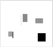
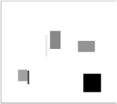
Figure 8: Top: original image of size $1024\times$ 1024 with a dynamic range of about $40$ dB. Bottom-Left: RecPF solution. Bottom-Right: NESTA solution.

The curves in Figure 9 show the number of calls to $A$ or $A^{*}$; mid-points are averages over $5$ random trials, with error bars indicating the minimum and maximum number of calls. Here, RecPF is stopped when

$$\|x_{\text{RecPF}}\|_{TV} \leq 1.05\|x_{N}\|_{TV},$$

$$\|b-Ax_{\text{RecPF}}\|_{\ell_{2}} \leq 1.05\|b-Ax_{N}\|_{\ell_{2}},$$

where $x_{N}$ is the solution computed via NESTA. As before continuation is very efficient when the dynamic range is high (typically higher than $40$ dB). An interesting feature is that the numbers of calls are very similar over all five trials. When the dynamic range increases, the computational costs of both NESTA and RecPF naturally increase. Note that in the $60$ and $80$ dB experiments, RecPF did not converge to the solution and this is the reason why the number of calls saturates. While both methods have a similar computational cost in the low-dynamic range regime, NESTA has a clear advantage in the higher-dynamic range regime. Moreover, the number of iterations needed to reach convergence with NESTA with continuation is fairly low—300-400 calls to $A$ and $A^{*}$—and so this algorithm is well suited to large scale problems.

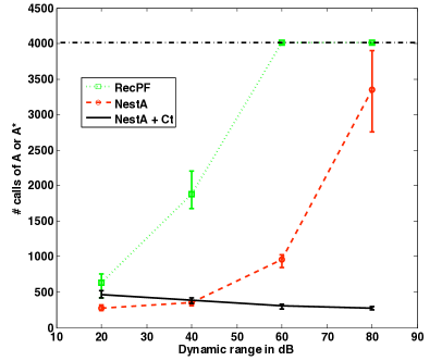
Figure 9: Number of calls to $A$ and $A^{*}$ as a function of the dynamic range. Solid line: NESTA with continuation. Dashed line: NESTA. Dotted line: RecPF. Dash-dotted: maximum number of iterations. In the $60$ and $80$ dB experiments, RecPF did not converge to the solution and this is the reason why the number of calls saturates.

7 Discussion

In this paper, we have proposed an algorithm for general sparse recovery problems, which is based on Nesterov’s method. This algorithm is accurate and competitive with state-of-the-art alternatives. In fact, in applications of greatest interest such as the recovery of approximately sparse signals, it outperforms most of the existing methods we have used in our comparisons and is comparable to the best. Further, what is interesting here, is that we have not attempted to optimize the algorithm in any way. For instance, we have not optimized the parameters $\{\alpha_{k}\}$ and $\{\tau_{k}\}$, or the number of continuation steps as a function of the desired accuracy $\delta$, and so it is expected that finer tuning would speed up the algorithm. Another advantage is that NESTA is extremely flexible in the sense that minor adaptations lead to efficient algorithms for a host of optimization problems that are crucial in the field of signal/image processing.

7.1 Extensions

This paper focused on the situation in which $A^{*}A$ is a projector (the rows of $A$ are orthonormal). This stems from the facts that 1) the most computationally friendly compressed sensing are of this form, and 2) it allows fast computations of the two sequence of iterates $\{y_{k}\}$ and $\{z_{k}\}$. It is important, however, to extend NESTA as to be able to cope with a wider range of problem in which $A^{*}A$ is not a projection (or not diagonal).

In order to do this, observe that in Steps $2$ and $3$, we need to solve problems of the form

$$y_{k}=\mathop{\mbox{argmin}}_{x\in\mathcal{Q}_{p}}\|x-q\|_{\ell_{2}}^{2},$$

for some $q$, and we have seen that the solution is given by $y_{k}=\mathcal{P}_{\mathcal{Q}_{p}}(q)$, where $\mathcal{P}_{\mathcal{Q}_{p}}$ is the projector onto $\mathcal{Q}_{p}:=\{x:\|Ax-b\|_{\ell_{2}}\leq\epsilon\}$. The solution is given by

$$y_{k}=(I+\lambda A^{*}A)^{-1}(q+\lambda A^{*}b)$$ (38)

for some $\lambda\geq 0$. When the eigenvalues of $A^{*}A$ are well clustered, the right-hand side of (38) can be computed very efficiently via a few conjugate gradients (CG) steps. Note that this is of direct interest in compressed sensing applications in which $A$ is a random matrix since in all the cases we are familiar with, the eigenvalues of $A^{*}A$ are tightly clustered. Hence, NESTA may be extended to general problems while retaining its efficiency, with the proviso that a good rule for selecting $\lambda$ in (38) is available; i.e. such that $\|Ay_{k}-b\|_{\ell_{2}}=\epsilon$ unless $q\in\mathcal{Q}_{p}$. Of course, one can always eliminate the problem of finding such a $\lambda$ by solving the unconstrained problem $(\text{QP}_{\lambda})$ instead of $(\text{BP}_{\epsilon})$. In this case, each NESTA iteration is actually very cheap, no matter how $A$ looks like.

Finally, we also observe that Nesterov’s framework is likely to provide efficient algorithms for related problems, which do not have the special $\ell_{1}+\ell_{2}^{2}$ structure. One example might be the Dantzig selector, which is a convenient and flexible estimator for recovering sparse signals from noisy data [15]:

$$\begin{array}[]{ll}\text{minimize}&\quad\|x\|_{\ell_{1}}\\ \text{subject to}&\quad\|A^{*}(b-AX)\|_{\ell_{\infty}}\leq\delta.\end{array}$$ (39)

This is of course equivalent to the unconstrained problem

$$\text{minimize}\quad\lambda\|x\|_{\ell_{1}}+\|A^{*}(b-AX)\|_{\ell_{\infty}}$$

for some value of $\lambda$. Clearly, one could apply Nesterov’s smoothing techniques to smooth both terms in the objective functional together with Nesterov’s accelerated gradient techniques, and derive a novel and efficient algorithm for computing the solution to the Dantzig selector. This is an example among many others. Another might be the minimization of a sum of two norms, e.g. an $\ell_{1}$ and a TV norm, under data constraints.

7.2 Software

In the spirit of reproducible research [26], a Matlab version of NESTA will be made available at: http://www.acm.caltech.edu/~nesta/

Acknowledgements

S. Becker wishes to thank Peter Stobbe for the use of his Hadamard Transform and Gabor frame code, and Wotao Yin for helpful discussions about RecPF. J. Bobin wishes to thank Hamza Fawzi for fruitful discussions, and E. Candès would like to thank Jalal Fadili for his suggestions. We are grateful to Stephen Wright for his comments on an earlier version of this paper, for suggesting to use a better version of GPSR, and encouraging us to test SpaRSA. Thanks Stephen!

References

- [1] J-F. Aujol, Some first-order algorithms for total-variation based image restoration, Journal of Mathematical Imaging and Vision (to appear), (2009).
- [2] J. Barzilai and J. Borwein, Two point step size gradient method, IMA Journal of Numerical Analysis, 8 (1988), pp. 141–148.
- [3] A. Beck and M. Teboulle, Fast iterative shrinkage-thresholding algorithm for linear inverse problems, SIAM J. Imaging Sciences, (2008).
- [4] A. Ben-Tal and A. Nemirovskii, Lectures on Modern Convex Optimization Analysis, and Engineering Applications, SIAM, Philadelphia, 2001.
- [5] J. M. Bioucas-Dias and M. A. T. Figueiredo, A new twist : two-step iterative shrinkage/thresholding algorithms for image restoration, IEEE Trans. On Image Processing, 16 (2007), pp. 2992–3004.
- [6] G. Birgin, J. M. Martinez, and M. Raydan, Nonmonotone spectral projected gradient methods on convex sets, SIAM Journal of Optimization, 10 (2000).
- [7] J. Bobin and E. J. Candès, A fast and accurate first-order algorithm for compressed sensing, submitted to ICIP09, (2009).
- [8] J. Bobin, J.-L. Starck, and R. Ottensamer, Compressed sensing in astronomy, Journal of Selected Topics in Signal Processing, 2 (2008), pp. 718–726.
- [9] J.-F. Cai, S. Osher, and Z. Shen, Linearized Bregman iterations for compressed sensing, Math. Comp. (to appear), (2008).
- [10] E. J. Candès, -magic, tech. report, Caltech, 2007.
- [11] E. J. Candès, L. Demanet, D. Donoho, and L. Ying, Fast discrete curvelet transforms, SIAM Multiscale Model. Simul, 5/3 (2006), pp. 861–899.
- [12] E. J. Candès and Y. Plan, Near-ideal model selection by minimization, Annals of Statistics - to appear, (2007).
- [13] E. J. Candès, J. Romberg, and T. Tao, Robust uncertainty principles: Exact signal reconstruction from highly incomplete frequency information, IEEE Trans. on Information Theory, 52 (2006), pp. 489–509.
- [14] E. J. Candès and T. Tao, Near optimal signal recovery from random projections: Universal encoding strategies?, IEEE Trans. on Information Theory, 52 (2006), pp. 5406–5425.
- [15] E. J. Candès and T. Tao, The Dantzig selector: statistical estimation when is much larger than , Annals of Statistics, 35 (2007).
- [16] E. J. Candès, M. B. Wakin, and S. P. Boyd, Enhancing sparsity by reweighted minimization, tech. report, Caltech, 2008.
- [17] A. Chambolle, An algorithm for total-variation minimization and applications, Journal of Mathematical Imaging and Vision, 20 (2004), pp. 89–97.
- [18] S. S. Chen, D. L. Donoho, and M. A. Saunders, Atomic decomposition by basis pursuit, SIAM Journal on Scientific Computing, 20 (1998), pp. 33–61.
- [19] P. L. Combettes and J. C. Pesquet, A proximal decomposition method for solving convex variational inverse problems, Inverse Problems, 24 (2008).
- [20] P. L. Combettes and V. R. Wajs, Signal recovery by proximal forward-backward splitting, SIAM Journal on Multiscale Modeling and Simulation, 4 (2005), pp. 1168–1200.
- [21] J. Dahl, C. Hansen, S. H. Jensen, and T. L. Jensen, Algorithms and software for total variation image reconstruction via first-order methods, submitted to Numerical Algorithms, (2008).
- [22] J. Darbon and M. Sigelle, A fast and exact algorithm for total-variation minimization, IbPRIA, 3522 (2005), pp. 351–359.
- [23] Analog-to-Information Receiver Development Program (A-to-I), 2007. DARPA Broad Agency Announcement (BAA) No. 08-03 available at http://www.darpa.mil/mto/Solicitations/baa08-03/index.html.
- [24] I. Daubechies, M. Defrise, and C. De Mol, An iterative thresholding algorithm for linear inverse problems with a sparsity constraint, Communications on Pure and Applied Mathematics, 57 (2004), pp. 1413–1457.
- [25] D. L. Donoho, Compressed sensing, IEEE Trans. on Information Theory, 52 (April 2006), pp. 1289–1306.
- [26] D. L. Donoho, A. Maleki, I. Rahman, M. Shahram, and V. Stodden, Fifteen years of reproducible research in computational harmonic analysis, preprint, (2008).
- [27] D. L. Donoho and Y. Tsaig, Fast solution of minimization problems when the solution may be sparse, Technical report, Stanford, (2006). submitted.
- [28] D. L. Donoho, Y. Tsaig, I. Drori, and J.-L. Starck, Sparse solution of underdetermined linear equations by stagewise orthogonal matching pursuit, IEEE Transactions On Information Theory, (2006). submitted.
- [29] M. Elad, P. Milanfar, and R. Rubinstein, Analysis versus synthesis in signal priors, Inverse Problems, 23 (2007), pp. 947–968.
- [30] M. A. Figueiredo and R.D. Nowak, An EM algorithm for wavelet-based image restoration, IEEE Trans. On Image Processing, 12 (2003), pp. 906–916.
- [31] M. A. Figueiredo, R. Nowak, and S. J. Wright, Gradient projection for sparse reconstruction: Application to compressed sensing and other inverse problems, IEEE Journal of Selected Topics in Signal Processing, 1 (2007), pp. 586 – 597.
- [32] J. Friedman, T. Hastie, and R. Tibshirani, Regularized paths for generalized linear models via coordinate descent. Technical Report, 2008.
- [33] T. Goldstein and S. Osher, The split Bregman method for l1 regularized problems, tech. report, UCLA department of mathematics, 2008.
- [34] E. T. Hale, W. Yin, and Y. Zhang, A fixed-point continuation method for l1-regularized minimization with applications to compressed sensing, Technical Report - Rice University, (2007).
- [35] E. T. Hale, W. Yin, and Y. Zhang, Fixed-point continuation for l1-minimization: Methodology and convergence, SIAM J. on Optimization, 19 (2008), pp. 1107–1130.
- [36] K. Koh, S. J. Kim, and S. Boyd, Solver for l1-regularized least squares problems, tech. report, Stanford University, 2007.
- [37] T. Lin and F. J. Herrmann, Compressed wavefield extrapolation, To appear in Geophysics, (2007).
- [38] M. Lustig, D. L. Donoho, and J. M. Pauly, Sparse MRI: The application of compressed sensing for rapid MR imaging, Magnetic Resonance in Medicine, 58 (2007), pp. 1182 – 1195.
- [39] S. Mallat, A Wavelet Tour of Signal Processing, Academic Press, 1998.
- [40] D. Needell and J. A. Tropp, Cosamp: Iterative signal recovery from incomplete and inaccurate samples, Appl. Comput. Harmon. Anal, 26 (2008).
- [41] Y. Nesterov, A method for unconstrained convex minimization problem with the rate of convergence , Doklady AN USSR (translated as Soviet Math. Docl.), 269 (1983).
- [42] , Introductory lectures on convex optimization: Basic course, Kluwer, Boston, 2003.
- [43] , Smooth minimization of non-smooth functions, Math. Program., Serie A, 103 (2005), pp. 127–152.
- [44] , Gradient methods for minimizing composite objective function, Technical Report - CORE - Universite Catholique de Louvain, (2007).
- [45] M. R. Osborne, B. Presnell, and B. A. Turlach, A new approach to variable selection in least squares problems, IMA Journal of Numerical Analysis, 20 (2000), pp. 389–403.
- [46] S. Osher, Y. Mao, B. Dong, and W. Yin, Fast linearized Bregman iteration for compressive sensing and sparse denoising, Comm. in Math. Sciences (to appear), (2008).
- [47] R. T. Rockafellar, Convex analysis, Princeton Landmarks in Mathematics and Physics, Princeton University Press, 1970.
- [48] M.A. Saunders and B. Kim, PDCO: Primal-dual interior method for convex objectives, tech. report, Stanford University, 2002. http://www.stanford.edu/group/SOL/software/pdco.html.
- [49] R. Tibshirani, Regression shrinkage and selection via the lasso, J. R. Statist. Soc. B., 58 (1996), pp. 267–288.
- [50] P. Tseng, On accelerated proximal gradient methods for convex-concave optimization, SIAM Journal of Optimization, (2008).
- [51] E. Van Den Berg and M. P. Friedlander, Probing the Pareto frontier for basis pursuit solutions, SIAM Journal on Scientific Computing, 31 (2008), pp. 890 – 912.
- [52] P. Weiss, L. Blanc-Féraud, and G. Aubert, Efficient schemes for total variation minimization under constraints in image processing, SIAM journal on Scientific Computing (to appear), (2009).
- [53] Z. Wen, W. Yin, D. Goldfarb, and Y. Zhang, A fast algorithm for sparse reconstruction based on shrinkage, subspace optimization and continuation, submitted to SIAM J. on Scientific Computing, (2009).
- [54] S. J. Wright, R. D. Nowak, and M. A. T. Figueiredo, Sparse reconstruction by separable approximation, IEEE Transactions on Signal Processing (to appear), (2009).
- [55] J. Yang, Y. Zhang, and W. Yin, A fast TV - minimization algorithm for signal reconstruction from partial Fourier data, Technical Report, TR08-27, CAAM, Rice University., (2008).
- [56] W. Yin, S. Osher, D. Goldfarb, and J. Darbon, Bregman iterative algorithms for minimization with applications to compressed sensing, SIAM J. Imaging Sciences, 1 (2008), pp. 143–168.