Depinning of a discrete elastic string from a two dimensional random array of weak pinning points

Abstract

The present work is essentially concerned with the development of statistical theory for the low temperature dislocation glide in concentrated solid solutions where atom-sized obstacles impede plastic flow. In connection with such a problem, we compute analytically the external force required to drag an elastic string along a discrete two-dimensional square lattice, where some obstacles have been randomly distributed. The corresponding numerical simulations allow us to demonstrate a remarkable agreement between simulations and theory for an obstacle density ranging from 1 to 50 $\%$ and for lattices with different aspect ratios. The theory proves efficient on the condition that the obstacle-chain interaction remains sufficiently weak compared to the string stiffness.

1 From the solid solution strengthening theory

The statistical theory for solid solution hardening (SSH) emerged from the seminal works of Sir N. Mott[1] and his near colleagues, F.R.N. Nabarro[2, 3] and J. Friedel [4]. The early analytical theory, perfected and extended by other contributors, as for instance R. Fleischer, R. Labusch and T. Suzuki [5, 6, 7, 8, 9] applies to substitutional alloys where the solute atoms can be considered as immobile during the dislocation glide, by contrast to the cases where dislocations may drag along an atmosphere of fast diffusing impurities. In face centered cubic (fcc) alloys, the critical resolved shear stress (CRSS) was then expected to increase in proportion to $c_{s}^{\eta}$ with $c_{s}$ as the atomic concentration of solute atoms and $\eta$ as an exponent depending on the assumptions made on the interaction between dislocations and foreign atoms: $\eta=1/2$ in Friedel-Fleischer (FF) theory while $\eta={2/3}$ in Mott-Nabarro-Labusch (MNL) theory and $\eta=1$ in Friedel-Mott-Suzuki (FMS) [4, 9]. Within analytical theory for SSH, the dislocation is thought of as a continuous elastic string impinged on a two-dimensional (2D) random static potential. The depinning transition in such a model is a typical issue of statistical physics, belonging to a broad class of problems concerned with extended interfaces motion in heterogeneous materials[10, 11, 12, 13, 14, 15, 16, 17, 18, 19, 20, 21, 22].

The recent developments of three-dimensional atomistic simulations (3D-AS) allowed to work on more realistic models for dislocations in solid solutions[23, 24, 25, 26, 27, 28, 29, 30]. Though 3D-AS confirmed that a large part of the dislocation pinning hinges on the impurities situated in the crystal planes that bounds the dislocation glide plane[23], the simulations revealed also the complexity of the dislocation-obstacle interaction. In fcc alloys, the geometry of the dislocation core, dissociated in two Shockley partials separated by a $(111)$ stacking fault ribbon undermines the simple picture of an elastic line in interaction with a single type of obstacles, as stated in the basic version of SSH theory. Instead, the pinning forces differ according to partials and to the obstacle positions, i.e., above or below the glide plane[25, 28].

On the other hand, the nanometric scale of the atomistic simulations, a stringent limit imposed by the computational load, hinders the direct extrapolation of simulation results to macroscopic samples. A multi-scale approach is thence required to link the atomistic studies to the realm of materials sciences. A manner to proceed consists in incorporating some of the atomic ingredients revealed in 3D-AS to a discrete version of the elastic string model that remains tractable even for large dimensions [31]. The discretization of the string model should allow to transfer of the atomic details.

In the present paper, the impact of the discretization on the depinning transition is analyzed thoroughly. The elastic string is replaced with a discrete spring chain, the nodes of which move on a 2D square lattice and interact with some pinning points randomly distributed on lattice sites. This very simple model allows us to devise an analytical theory which accounts for the discreteness of the obstacle distribution and thus opens a promising perspective to integrate more of the atomic details. In order to demonstrate the accuracy of the theory, we compute directly the critical external force within numerical simulations applied to the discrete string model. Theory and simulations agree remarkably well for a broad range of model parameters, e.g., (i) the in-plane obstacle density $c_{s}$, (ii) the lattice size in every direction of space, (iii) the maximum pinning force $f_{M}$ and (iv) the potential interaction cutoff $w$ that characterizes the obstacles. The theoretical predictions are proved reliable on the condition that $f_{M}$ and $w$ remain smaller than certain bounds varying with $c_{s}$. For a dense distribution of weak pinning points, the critical configuration of the chain is found to be a quasi-straight line parallel to the atomic rows. The depinning is then shown to occur at some vacant site clusters (VSC) which the typical size is explicitly related to the lattice dimensions in both directions of space. The external force required to drag along the spring chain over a finite distance reflects such a size dependence. Noteworthily the effective density exponent $\eta$ is also found to vary with lattice dimensions, in contrast with expectations drawn on standard SSH theory.

Our report is organized as follows. In Sec. II, the spring chain model is introduced and the direct numerical computations are described. In Sec. III, the statistical theory is derived and compared to the numerical data. The results are resumed and commented in Sec. IV.

2 The phenomenological spring chain model

The model proposed hereafter belongs to the wide class of elastic interface models, extensively studied in statistical physics [16, 17, 18, 19, 20, 21, 22]. A one dimensional elastic string is discretized with a spatial step $b$, equivalent to the shortest interatomic distance in solids. Each node of the discrete chain is bound to its first neighbor by an harmonic spring of strength $\Gamma$. The two quantities, $b$ and $\Gamma$ are chosen to scale distances and forces, respectively. The spring chain nodes move along the column of a square lattice. The size of the lattice in the direction of the chain is denoted as $L_{y}$ whereas the distance over which the chain is dragged is $L_{x}$. The 2D random array of obstacles is constructed by selecting the occupied lattice sites, up to a number of obstacle equals to $c_{s}L_{x}L_{y}$, where $c_{s}$ is the obstacle density. Since the depinning process occurs when the chain nodes pass the force maximum, the interaction potential is expended as a polynomial function in the vicinity of such a maximum. Assuming that the interaction is attractive and that the potential is symmetric with respect to its minimum, we obtain a polynomial function of at least fourth order:

$$V(x) = V_{0}({x^{2}}/{w^{2}}-1)^{2}\ \text{for}\ |x|<w$$

$$V(x) = 0\ \text{for}\ |x|>w,$$ (1)

which corresponds to a force $f(x)=-4V_{0}({x^{2}}/{w^{2}}-1){x}/{w^{2}}$, with a maximum value $f_{M}=8|V_{0}|/(3\sqrt{3}w)$, attained when $x=\pm w/\sqrt{3}$. The chain nodes interact solely with obstacles situated in the column along which they may glide. The polynomial force with a distance cutoff $w$ is obviously very far from the dislocation-solute interaction, characterized by a decrease of Coulomb type. Hereby we describe only the local potential variation yielded when a solute atom visits a dislocation core. The parameter $w$ fixes how the interaction decreases in the vicinity of the force maximum. Both $f_{M}$ and $w$ can be extracted from atomistic data as those reported in [25, 28].

The dimensionless over-damped Langevin dynamics for the chain node $k$ is given by:

$$\dot{x_{k}}=[x_{k+1}+x_{k-1}-2x_{k}]+\tau-\sum_{i}4V_{0}\frac{(x_{k}-s_{k,i})}{w^{2}}(\frac{(x_{k}-s_{k,i})^{2}}{w^{2}}-1),$$ (2)

where $x_{k}$ is the position of the node $k$, $\tau$ is the external force and $s_{k,i}$ is the coordinate of the ith obstacle in the kth row. For the weak pinning forces we are concerned with, the chain strain remains very small such that the anharmonic terms in the spring tension have been neglected. Properly scaled, the continuous version of the spring chain model served in the development of the SSH theory [1, 3, 4, 8].

In the direct numerical simulations of Eq. 2, $\tau$ is incremented adiabatically in the course of the integration of the chain motion. Once [$\sup_{k}|\dot{x_{k}}|$] is inferior to a certain precision (i.e., $10^{-7}$) the external force is incremented. Before each increment, the chain configuration is recorded and once the chain has run over a distance $L_{x}$, the integration is stopped. The latest anchored configuration corresponds to the strongest one and the associated external force is denoted as $\tau_{c}$, i.e., the static depinning threshold. We performed this type of simulations for different lattice aspect ratios, varying $L_{x}$ and $L_{y}$ and for different obstacle densities ranging from 1 to 50 $\%$. Various algorithms for the random numbers generator needed to build the obstacle array were tested and no significant difference was noticed in the end results.

Figure 1: (color online) Strongest pinning configuration of the spring chain on a random array of obstacles (circles) for $f_{M}=0.1$, $L_{y}=2000$, $L_{x}=500$, a density $c_{s}=16$ $\%$ and an interaction cutoff $w=1$. Only obstacles close from the chain have been reported for clarity. Inset shows a magnification of obstacles (circles) and nodes (triangles) of a chain segment. X and Y axis have different scaling for convenience of the plot.

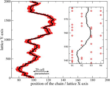
In Fig. 1, we report the strongest chain configuration, obtained from the numerical simulations for a pinning strength $f_{M}=0.1$. The critical profile is found to be wavy and to cross at least 40 lattice rows. In Figs. 2 (a) and (b), the critical chain profile is shown for smaller values of $f_{M}$, i.e., two orders of magnitude smaller than the one used in Fig. 1. We note that the entire string length is bounded by only two rows. The simulations evidence actually a well known feature for pinning of extended defects, namely weaker the obstacles flatter the shape of the critical configuration. A perfectly rigid string would even experience a null force since then $f_{M}$ would be negligible compared to the spring tension. However, as soon as some elasticity enters into play, the pinning strength becomes positive. The present work is essentially concerned with cases like those presented in Figs. 2 (a) and (b), where the elastic string shape is quasi-straight. In such situations, the string roughness is inferior or of the order of the inter-atomic spacing. The result shown in Fig. 1 only served us for comparison in order to introduce our problem. Such a case of wavy critical profile has been studied extensively, both through numerical simulations[32, 33, 34, 35, 36] and analytical works [5, 6, 7, 8].

Figure 2: (color online) Strongest pinning configuration on a random array of obstacles (circles) for a chain length $L_{y}=2000$ and a drag distance $L_{x}=500$. In (a) the interaction cutoff is $w=0.5$, the obstacle strength $f_{M}=0.005$ and the obstacle density $c_{s}=7$ $\%$. In (b) $w=1$, $f_{M}=0.001$ and $c_{s}=9$ $\%$. In the insets some segments are magnified with chain nodes marked as triangles (not visible on the main graphics). The X and Y axis scales differ for convenience of the plot.

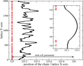
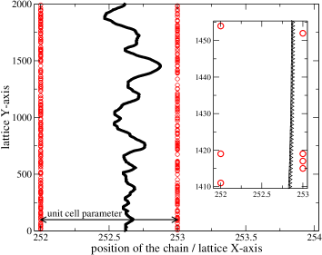
In the insets shown in Figs. 2 (a) and (b), it is worth noticing that along the rows that bound the spring chain, some holes appear in the obstacle distributions. Hereafter, we dubbed such holes vacant site clusters. The sampling of such density fluctuations along lattice rows plays a key role in the determination of the critical drag force.

3 Vacant site cluster sampling theory

3.1 The tightly bound chain

In Fig. 2 (a), we noticed that for some parameters the strongest configuration of the spring chain remains tightly bound to the single lattice row at the back of the chain, i.e., most of the chain nodes are closer from the back row than from the next nearest one and thereby the chain does not cross several lattice rows. In the present section, a theory is devised to compute the critical drag force corresponding to critical configurations like the one shown in Fig. 2 (a). Further, the theory will be extended to cases with broader interaction cutoff.

When the chain is tightly bound to the back row, the string can be viewed as quasi-straight, notwithstanding the bulges formed between rows. When $w\leq 0.5$, we can assume that the chain interacts with rows one by one and it is natural to work on the hypothesis that for such a system the strength of the random lattice is fixed by its more crowded row. To translate such a remark into some algebra, one needs to study the sampling of obstacles on a finite size lattice $L_{x}\times L_{y}$. We notice that the purely random planar distribution follows Bernoulli’s binomial law and the number of obstacles $N_{o}$ involved into a single row of length $L_{y}$ is then a random variable which probability is given by:

$$\rho(N_{o})=\mathds{C}_{N_{o}}^{L_{y}}\ c_{s}^{N_{o}}\ (1-c_{s})^{L_{y}-N_{o}},$$ (3)

where $\mathds{C}_{N_{o}}^{L_{y}}={L_{y}!}/{N_{o}!(L_{y}-N_{o})!}$. Such a statistical distribution can be approximated with a Poisson law in the limit of large $L_{y}$. However such a rounding yields some error for smallest $L_{y}$ we are concerned with, so we keep the binomial formulation of Eq. 3. The probability for a row to involve less than $N$ obstacles is $\sum_{N_{o}<N}\rho(N_{o})$ and therefore in a set of $L_{x}$ rows the probability for having a row with $N_{m}$ obstacles and $(L_{x}-1)$ rows with a number of obstacles inferior to $N_{m}$ is :

$$\beta(N_{m})=L_{x}\ [\rho(N_{m})]\ [\sum_{N_{o}<N_{m}}\rho(N_{o})]^{L_{x}-1}.$$ (4)

The maximum number $N_{m}$ fixing the number of obstacles in the denser row depends only on the lattice dimensions in each direction of space and on the overall obstacle density $c_{s}$. It is easily computed numerically, paying attention to avoid overflows in factorials computation. The mean density in the denser row is then $c_{m}=N_{m}/L_{y}$. When an excess of vacant sites emerges at some place along the denser row, such segment is weaker than others where the obstacles are more crowded. Thence the spring chain should start the crossing at the largest vacant site clusters (VSC). The typical size of such VSC must now be determined. Actually the mean number of VSC in a row which obstacle density is fixed to $c_{m}$ is $L_{VSC}=(c_{m}L_{y}-1)\approx N_{m}$. The normalized probability to find a VSC with exactly n vacant sites is $c_{m}(1-c_{m})^{n}$ while the probability for a VSC which size is inferior to $n$ is $[1-(1-c_{m})^{n}]$. The probability to find a VSC of size n and ($L_{VSC}-1$) VSC with size inferior to n is proportional to:

$$\gamma(n)=L_{VSC}\ [c_{m}(1-c_{m})^{n}]\ [1-(1-c_{m})^{n}]^{L_{VSC}-1}.$$ (5)

The mean size of the largest VSC in the denser row is thus:

$$n_{v}=\sum_{n}[n\gamma(n)]/\sum_{n}\gamma(n).$$ (6)

Such a maximum VSC is surrounded by other VSC’s that mean size is given by: $[\sum_{n<n_{v}}nc_{m}(1-c_{m})^{n}]/[\sum_{n<n_{v}}c_{m}(1-c_{m})^{n}]$ which for convenience is denoted as $(m-1)$ with:

$$m=\frac{1}{c_{m}}-n_{v}\frac{(1-c_{m})^{n_{v}}}{1-(1-c_{m})^{n_{v}}}.$$ (7)

To compute the external force associated with the strongest binding row we consider the segment of $n_{v}$ vacant sites as embedded into a regular lattice of obstacles spaced by a mean distance $m$. Such a mean-field construction is illustrated within Fig. 3, where spring chain’s nodes (triangles) are bound to the lattice sites occupied by the obstacles (large open circles).

Figure 3: (color online) Schematic representation of the model used for a quasi-straight spring chain tightly bound to a single lattice row. The small full circles represent the lattice sites, the large open circles represent the obstacles and the triangles are for the spring chain nodes. The average number $n_{v}$ of vacant sites involved in the largest vacant site cluster is determined through Eq. 6 and Eq. 5. The average spacing $m$ between the obstacles on both sides of the largest vacant site cluster is fixed by Eq. 7.

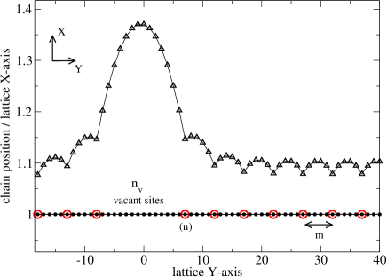
The array of obstacles is assumed to be centro-symmetric, so we ascribe the label 0 to the center of symmetry which corresponds to the top of the bulge. We also define a new variable $n=(1+n_{v})/2$ for convenience of the notations. Under the external applied force $\tau$, The force balance sheet, for say the left hand side of the chain leads to the set of equations:

$$F_{0} = -\tau-2(x_{1}-x_{0})$$

$$F_{1} = -\tau-(x_{2}+x_{0}-2x_{1})$$

$$F_{2} = -\tau-(x_{3}+x_{1}-2x_{2})$$

. $$=$$ .

$$F_{n-1} = -\tau-(x_{n}+x_{n-2}-2x_{n-1})$$

$$F_{n} = -\tau-f(x_{n})-(x_{n+1}+x_{n-1}-2x_{n})$$

$$F_{n+1} = -\tau-(x_{n+2}+x_{n}-2x_{n+1})$$

. $$=$$ .

$$F_{n+m-1} = -\tau-(x_{n+m}+x_{n+m-2}-2x_{n+m-1})$$

$$F_{n+m} = -\tau-f(x_{n+m})-(x_{n+m+1}+x_{n+m-1}-2x_{n+m})$$

$$F_{n+m+1} = -\tau-(x_{n+m+2}+x_{n+m}-2x_{n+m+1}),$$ (8)

and in principle the series of equations repeats up to the chain boundaries with increment of subscripts. We assume that the mechanical equilibrium is satisfied for all nodes $j$ situated in between obstacles. Then we have $F_{j}=0$ but for $j\in[n,n+m,..n+pm]$. For the segment $j\in[0,n]$, it is easy to show by recurrence that : $x_{j}-x_{0}=-\tau j^{2}/2$. Thence the chain shape is parabolic between $n$ and $-n$. For $j\in[n,n+m]$, we proceed the same and find $x_{j+n}-x_{n}=-\tau j(n+j/2)-[F_{n}+f(x_{n})]j$ which fixes the segment end to

$$x_{n+m}=x_{n}-\tau m(n+m/2)-m[F_{n}+f(x_{n})].$$ (9)

The same can be iterated once again for $j\in[n+m,n+2m]$ which leads to $x_{n+2m}-x_{n+m}=-\tau m(n+3m/2)-(F_{n}+F_{n+m}+f(x_{n})+f(x_{n+m}))m$. The set of equation on the positions $x_{n+jm}$ is then:

$$x_{n+m} = x_{n}-\tau m(n+m/2)-f(x_{n})m$$

$$x_{n+2m} = x_{n+m}-\tau m(n+3m/2)-[F_{n}+F_{n+m}+f(x_{n})+f(x_{n+m})]m$$

. $$=$$ .

. $$=$$ .

$$x_{n+pm} = x_{n+(p-1)m}-\tau m(n+(2p-1)\frac{m}{2})-m\sum_{j=0}^{p-1}[F_{n+jm}+f(x_{n+jm})].$$ (10)

Subtracting the two latest equations yields:

$$F_{n+pm}=-\frac{\Delta_{m}x_{n+pm}}{m}-\tau m-f(x_{n+pm})$$ (11)

where $\Delta_{p}x_{n+pm}=(x_{n+(p+1)m}+x_{n+(p-1)m}-2x_{n+pm})$ is the discrete Laplacian applied to the p subscript. When the entire chain is at mechanical equilibrium $F_{n+pm}=0$ for all $p$. Far enough from the $n_{v}$-VSC (i.e., the VSC with $n_{v}$ vacant sites), the solution for $x_{n+pm}$ tends asymptotically to a constant $x_{\infty}$ such as $\tau m=-f(x_{\infty})$ and therefore:

$$x_{\infty}=\frac{2}{\sqrt{3}}\cos(\frac{\arccos(-\tau m/f_{M})}{3}+\frac{4\pi}{3}).$$ (12)

We can expend linearly Eq. 11 for the far enough sites such as the displacement $x_{n+pm}$ writes $x_{n+pm}=x_{\infty}+\epsilon_{p}$ and $f(x_{n+pm})=f(x_{\infty})+f^{\prime}(x_{\infty})\epsilon_{p}$. Then, at the equilibrium Eq. 11 yields $[\Delta_{p}\epsilon_{p}=-f^{\prime}(x_{\infty})m\epsilon_{p}]$ and thence $\epsilon_{p}$ is an exponential function: $[\epsilon_{p}=\epsilon_{0}\exp(-\alpha p)]$ which the exponent $\alpha$ verifies

$$\alpha=\pm 2\operatorname{ash}(\sqrt{-f^{\prime}(x_{\infty})m}/2).$$ (13)

Since the chain displacement is bounded, we are solely concerned with solutions such as $(\alpha p)>0$. The sum of the whole set of equations in Eq. 10 provides another relation between $\tau$ and the nodes position $x_{n+pm}$, on the condition that $F_{n+pm}=0$ for all $p$:

$$x_{n}-x_{n+pm}=m[\tau p(n+pm/2)+\sum_{j=0}^{p-1}(p-j)f(x_{n+jm})],$$ (14)

which after expanding $f(x_{n+jm})$ as a Taylor series around $x_{\infty}$ and keeping only the terms linear in p provides us with an equation which relates $\tau$ to $\epsilon_{0}$:

$$\tau=\frac{-\epsilon_{0}}{(n-m/2)}[\frac{f^{\prime}(x_{\infty})}{(1-e^{-\alpha})}+\frac{\epsilon_{0}f^{\prime\prime}(x_{\infty})}{2(1-e^{-2\alpha})}+\frac{\epsilon_{0}^{2}f^{\prime\prime\prime}(x_{\infty})}{6(1-e^{-3\alpha})}].$$ (15)

The critical chain configuration is reached when the Hessian associated with Eq. 11 has a singular eigenvalue. This allows us to determine the critical value for $\epsilon_{0}$. Actually we found that finding the Hessian singular eigenvalue is equivalent to find the maximum of Eq. 15 for $\tau$ with respect to $\epsilon_{0}$. The solution for the critical bulge is then:

$$\epsilon_{0}=-3(1-e^{-3\alpha})\frac{f^{\prime\prime}(x_{\infty})-\sqrt{f^{\prime\prime}(x_{\infty})^{2}-4f^{\prime\prime\prime}(x_{\infty})f^{\prime}(x_{\infty})\frac{(1-e^{-2\alpha})^{2}}{3(1-e^{-3\alpha})(1-e^{-\alpha})}}}{2f^{\prime\prime\prime}(x_{\infty})(1-e^{-2\alpha})}.$$ (16)

Combining the solutions for Eqs. 12, 13, 15 and 16 allows us to determine the maximum pinning force associated with $N_{m}$, the number of obstacle in the denser row. For this reason, we denote such a maximum as $\tau(N_{m})$. The set of equations giving $\tau(N_{m})$ can be solved recursively. Starting with a small enough trial solution for $\tau=\tau_{0}$, we compute the corresponding quantities $x_{\infty}$ and $\alpha$ from Eq. 12 and from Eq. 13. Then $\epsilon_{0}$ is derived from Eq. 16 and the corresponding value of $\tau$ from Eq. 15. If the so obtained quantity is larger than the initial value $\tau_{0}$ then the latter is incremented and we proceed the same up to find identical values for $\tau$ and $\tau_{0}$. The end result gives the required $\tau(N_{m})$ to a precision fixed by the trial solution increment.

Figure 4: (color online) External force required to drag a spring chain of length $L_{y}$ over a distance $L_{x}$, for a pinning strength $f_{M}=0.005$ and a cutoff $w=0.1$ in (a) and $w=0.5$ in (b). The symbols represent the data obtained through the simulations described in Sec. 2, for different lattices (see figures legend). The continuous lines correspond to the predictions made through the theory detailed in Sec. 3 for same parameters as those used in simulations. Colors of symbols and lines correspond one to one.

The critical pinning force $\tau_{c}$ of the random lattice is approximated by averaging $\tau(N_{m})$ over $N_{m}$:

$$\tau_{c}=\sum_{N_{m}}\beta(N_{m})\tau_{c}(N_{m}),$$ (17)

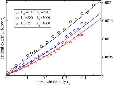
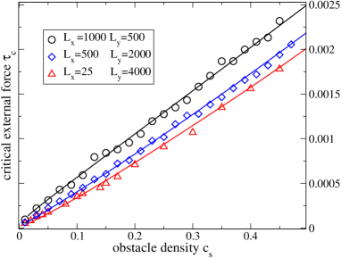
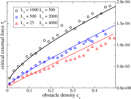
where $\beta(N_{m})$ has been given in Eq. 4. The previous theory is compared to simulations data in Figs. 4 (a) and (b) and in Fig. 5 for different lattice dimensions, different pinning forces, varying $w$ and $f_{M}$. A quantitative agreement has been obtained between theory and simulations, although no adjustable parameters are involved. According to same type of comparisons but for larger $f_{M}$ values, the previous analytical work proves relevant for $f_{M}$ smaller than roughly $0.03$.

Figure 5: (color online) External force required to drag a spring chain of length $L_{y}=1000$ along a distance $L_{x}=100$, for different obstacle pinning strengths (see legend) and the same interaction range $w=0.5$. The different symbols represent the simulations data and the continuous lines correspond to the prediction made through the analytical theory detailed in Sec. 3 for same parameters.

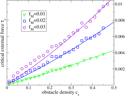
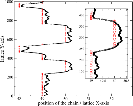
The theory predictions worsen for cases where the critical configuration crosses few lattice rows. As an example, for $f_{M}=0.03$ in Fig. 5, the VSC theory is found to become less accurate for low densities. In such conditions, the string profile at the depinning transition corresponds to a kinked shape, as shown in Fig. 6, different from the wavy profile shown in Fig. 1 and from the quasi-straight ones shown in Figs. 2 (a) and (b). From Fig. 5, it can be seen that the discrepancy increases as the density decreases while the theoretical predictions remain accurate for more concentrated obstacle distributions. As $f_{M}$ increases above $0.03$, the deviation between theoretical predictions and simulations data is shifted toward higher densities. In this range of parameters, the system undergoes a bifurcation, not treated in the present work.

Figure 6: (color online) Strongest pinning configuration for $f_{M}=0.03$, $L_{y}=1000$, $L_{x}=100$, a density $c_{s}=9$ $\%$ and an interaction cutoff $w=0.5$. The inset shows a chain segment the nodes of which are marked with triangles. Only obstacles close from the string have been reported as circles.

Other authors [32, 33] noticed that the maximum pinning force of a random lattice was dependant of the drag distance. Concerning the weak pinning points studied here, it is thus of some interest to explore the variation of the critical drag force with lattice dimensions. The critical drag force was found to vary proportionally to $[\ln(L_{x})]^{\alpha_{x}}$ where $\alpha_{x}$ varies with all parameters. For instance when $w=0.5$, $f_{M}=0.01$ and $L_{y}=1000$, we found $\alpha_{x}=[0.45-0.036\ln(c_{s})]$. One can thus conclude that the $L_{x}$ dependence is very weak since a fractional power of a logarithm is a rather wise function. The maximum drag force depends not only on $L_{x}$ but also on $L_{y}$. The critical drag force varies proportionally to a constant plus the function $[\ln(L_{y})]^{-\alpha_{y}}$ where $\alpha_{y}$ decreases when $c_{s}$ increases. For instance when $w=0.5$, $f_{M}=0.01$ and $L_{x}=4000$, we found $\alpha_{y}=[0.26-0.63\ln(c_{s})]$. According to direct simulations, the $\tau_{c}$ dependence in $L_{y}$ seems to weaken when $f_{M}$ becomes large enough for the critical configuration to differ from the quasi-straight line as in Fig. 6 or Fig. 1.

For fixed lattice dimensions, the adjustment of a density power law for the theoretical critical drag force allows to establish some comparison with the SSH analytical theory. The density power law fit is found very close from a linear variation and may even overpass slightly the unitary exponent in some situations depending on the lattice geometry. For instance, from Fig. 4 (b), we worked out by a curve fitting with the form $\tau_{c}\propto(c_{s}^{\eta})$, an exponent $\eta=1.13$ for $L_{y}=4000$ and $L_{x}=25$ whereas for $L_{y}=500$ and $L_{x}=1000$, $\eta=0.946$ was obtained. The effective density exponent $\eta$ is therefore size dependent. A density exponent close from unity corresponds to the FMS theory for the hardening of concentrated solid solutions. The CRSS linear dependence in the solute concentration was also noted in atomistic calculations on the model solid solution Ni(Al) [28].

3.2 Extension to broader cutoff

To extend the theory developed previously for a short cutoff $w$, we first consider the case $w\approx 1$, which allows us to treat the spring chain interaction with only two rows: the row at the back and the next nearest one. Such a critical configuration can be seen from direct simulations as reported in Fig. 2 (b). To compute $\tau_{c}$, we still employ the same model as depicted in Fig. 3. However, the interaction with the next nearest row may weaken the pinning on the back row. One ascribes to each site $j$ of the next nearest row, a force $g(x_{j})=c_{v}f(x_{j}-1)$ where $c_{v}$ is the density of obstacles in the next nearest row. For the situation shown in Fig. 3, the force balance sheet writes as follows:

$$F_{0} = -\tau-g(x_{0})-2(x_{1}-x_{0})$$

$$F_{1} = -\tau-g(x_{1})-(x_{2}+x_{0}-2x_{1})$$

$$F_{2} = -\tau-g(x_{2})-(x_{3}+x_{1}-2x_{2})$$

. $$=$$ .

$$F_{n-1} = -\tau-g(x_{n-1})-(x_{n}+x_{n-2}-2x_{n-1})$$

$$F_{n} = -\tau-g(x_{n})-f(x_{n})-(x_{n+1}+x_{n-1}-2x_{n})$$

$$F_{n+1} = -\tau-g(x_{n+1})-(x_{n+2}+x_{n}-2x_{n+1})$$

. $$=$$ .

$$F_{n+m-1} = -\tau-g(x_{n+m-1})-(x_{n+m}+x_{n+m-2}-2x_{n+m-1})$$

$$F_{n+m} = -\tau-g(x_{n+m})-f(x_{n+m})-(x_{n+m+1}+x_{n+m-1}-2x_{n+m})$$

$$F_{n+m+1} = -\tau-g(x_{n+m+1})-(x_{n+m+2}+x_{n+m}-2x_{n+m+1})$$

. $$=$$ . (18)

To estimate the force exerted by the next nearest row upon the spring chain, the function $g(x_{j})$ is approximated with a step function: $g(x_{j})=g(x_{0})$ if $j\in[0;n-(m-1)/2[$ and $g(x_{j})=g(x_{n+pm})$ if $j\in[n+pm-(m-1)/2;n+pm+(m+1)/2[$. We then assume that the mechanical equilibrium is achieved for all nodes excepted those aligned with some obstacles of the back row. This leads then to the following set of equations:

$$\tau = -g(x_{0})-2(x_{1}-x_{0})$$

$$\tau = -g(x_{0})-(x_{2}+x_{0}-2x_{1})$$

. $$=$$ .

$$\tau = -g(x_{n})-(x_{n}+x_{n-2}-2x_{n-1})$$

$$F_{n} = -\tau-f(x_{n})-g(x_{n})-(x_{n+1}+x_{n-1}-2x_{n})$$

$$\tau = -g(x_{n})-(x_{n+2}+x_{n}-2x_{n+1})$$

. $$=$$ .

$$\tau = -g(x_{n+m})-(x_{n+m}+x_{n+m-2}-2x_{n+m-1})$$

$$F_{n+m} = -\tau-f(x_{n+m})-g(x_{n+m})-(x_{n+m+1}+x_{n+m-1}-2x_{n+m})$$

$$\tau = -g(x_{n+m})-(x_{n+m+2}+x_{n+m}-2x_{n+m+1}),$$ (19)

and the equations repeat up to the chain boundaries by incrementing subscripts. By applying recurrence, it is possible to reduce the previous set of equations to a smaller one, concerning only the regular array of obstacles in the back row:

$$x_{n+pm} = x_{n+(p-1)m}-\tau m(n+(2p-1)m/2)-m\big{[}\sum_{j=0}^{p-1}[F_{n+jm}+f(x_{n+jm})]$$ (20)

$$+m\sum_{j=0}^{p-2}g(x_{n+jm})+g(x_{0})(n-m/2)\big{]}-\frac{m^{2}-1}{8}g(x_{n+pm})$$

$$-m\frac{3m-1}{4}g(x_{n+(p-1)m}).$$

Subtracting the equation for rank ($p-1$) from the one at rank ($p$) gives:

$$F_{n+pm} = -\Delta_{m}x_{n+pm}-\tau m^{2}-mf(x_{n+pm})$$ (21)

$$-\frac{m^{2}-1}{8}\big{[}g(x_{n+(p+1)m})+g(x_{n+(p-1)m})\big{]}-\frac{3m^{2}+1}{4}g(x_{n+pm}),$$

while for $p=0$:

$$F_{n} = x_{n}-x_{n+m}-\tau m(n+m/2)-m[f(x_{n})+g(x_{0})(n-m/2)]$$ (22)

$$-\frac{m^{2}-1}{8}g(x_{n+m})-m\frac{3m-1}{4}g(x_{n}).$$

When the equilibrium is achieved $F_{n+pm}=0$ for all p, which allows us to deduce the asymptotical solution of Eq. 21 as a constant $x_{n+pm}\rightarrow x_{\infty}$ which verifies:

$$\tau m=-f(x_{\infty})-mg(x_{\infty}).$$ (23)

The solution to Eq. 23 is the positive real root of a third order polynomial equation:

$$x_{\infty} = \frac{mc_{v}}{1+mc_{v}}+\sqrt{\frac{-2A_{\infty}}{3}}\cos{\big{(}\arccos{\big{(}\frac{-B_{\infty}}{2}\sqrt{\frac{27}{-A_{\infty}^{3}}}}\big{)}/3+\frac{4\pi}{3}\big{)}}$$ (24)

$$\text{with}\ A_{\infty}=\frac{1}{1+mc_{v}}\big{[}\frac{3mc_{v}}{w^{2}}-1-mc_{v}-\frac{3(mc_{v})^{2}}{w^{2}(1+mc_{v})}\big{]}$$

$$\text{and}\ B_{\infty}=\frac{1}{1+mc_{v}}\big{[}\frac{mc_{v}(\frac{3mc_{v}}{w^{2}}-mc_{v}-1)}{w(1+mc_{v})}-2\frac{(mc_{v})^{3}}{w^{3}(1+mc_{v})^{2}}$$

$$\text{\vspace{2.cm} \ \ \ \ \ \ \ \ }+\frac{2m\tau}{3f_{M}\sqrt{3}}-\frac{(mc_{v})}{w^{2}}(1/w^{2}-1)\big{]}.$$

If $(1-x_{\infty})>w$ then we can set $c_{v}=0$ in the previous equation which leads to Eq. 12, valid for small $w$.

Figure 7: (color online) Same as in Fig.4 but for a cutoff $w=1$ and a pinning strength $f_{M}=0.001$.

We now expend linearly Eq. 21 around $x_{\infty}$ to determine an approximation of nodes position as $x_{n+pm}=x_{\infty}+\epsilon_{p}$. The equation on $\epsilon_{p}$ is:

$$\Delta_{1}\epsilon_{p}=-mf^{\prime}(x_{\infty})\epsilon_{p}-\frac{3m^{2}+1}{4}g^{\prime}(x_{\infty})\epsilon_{p}-\frac{m^{2}-1}{8}g^{\prime}(x_{\infty})\big{[}\epsilon_{p+1}+\epsilon_{p-1}\big{]}.$$ (25)

The solution is an exponential function $\epsilon_{p}=\epsilon_{0}\exp(-\alpha p)$ with a dispersion relation:

$$\alpha=\pm\operatorname{ach}{\big{(}\frac{2-mf^{\prime}(x_{\infty})-(3m^{2}+1)g^{\prime}(x_{\infty})/4}{2+\frac{m^{2}-1}{4}g^{\prime}(x_{\infty})}\big{)}}.$$ (26)

At this stage, it is of some interest to work out the maximum of the spring chain position. For the segment situated along the larger hole (see Fig. 3), $j\in[0,n-(m-1)/2[$, the set of very first equations in Eqs. 19 leads to:

$$x_{n}-x_{0} = -\frac{\tau n^{2}}{2}-\frac{m^{2}-1}{8}g(x_{n})-\frac{g(x_{0})}{2}[n^{2}-m^{2}/4+1/4].$$ (27)

Then $x_{0}$ can be expressed as a function of $x_{n}$ since $x_{0}$ is actually the positive root of a third order polynomial:

$$x_{0} = 1+2w\sqrt{\frac{A_{0}+w}{3A_{0}}}\cos{\big{[}\arccos{\big{(}-\frac{C_{0}}{2A_{0}}\sqrt{\frac{27A_{0}^{3}}{(A_{0}+w)^{3}}}\big{)}}/3+4\pi/3\big{]}}$$ (28)

$$\text{with}\ A_{0}=\frac{2V_{0}c_{v}}{w}\big{[}n^{2}-m^{2}/4+1/4\big{]},$$

$$\text{and}\ C_{0}=x_{n}-1+\frac{\tau n^{2}}{2}+\frac{m^{2}-1}{8}g(x_{n}).$$

We also need to express the first derivative of $x_{0}$ against $x_{n}$ which according to Eq. 27 gives:

$$\frac{dx_{0}}{dx_{n}}=\frac{1+\frac{m^{2}-1}{8}g^{\prime}(x_{n})}{1-[n^{2}-(m^{2}-1)/4]g^{\prime}(x_{0})/2}.$$ (29)

The sum of the equations in Eq. 20 from rank 1 to rank p, taken sufficiently large, leads to an equation which the linear term in p is:

$$\tau= -g(x_{0})+\frac{1}{[n-m/2]}\big{[}\frac{(m+1)^{2}}{8m}g(x_{\infty})-\epsilon_{0}\frac{(f^{\prime}(x_{\infty})+mg^{\prime}(x_{\infty}))}{1-e^{-\alpha}}$$ (30)

$$-\epsilon_{0}^{2}\frac{(f^{\prime\prime}(x_{\infty})+mg^{\prime\prime}(x_{\infty}))}{2(1-e^{-2\alpha})}-\epsilon_{0}^{3}\frac{(f^{\prime\prime\prime}(x_{\infty})+mg^{\prime\prime\prime}(x_{\infty}))}{6(1-e^{-3\alpha})}\big{]}.$$

The latter equation is similar to Eq. 15 obtained for the tightly bound chain, but includes the interaction with the next nearest row. The maximum $\tau$ in Eq. 30 against $\epsilon_{0}$ corresponds to the critical strength which provides a transcendental equation on $\epsilon_{0}$:

$$[n-m/2]g^{\prime}(x_{0})\frac{dx_{0}}{dx_{n}}= -\frac{(f^{\prime}(x_{\infty})+mg^{\prime}(x_{\infty}))}{1-e^{-\alpha}}-\epsilon_{0}\frac{(f^{\prime\prime}(x_{\infty})+mg^{\prime\prime}(x_{\infty}))}{(1-e^{-2\alpha})}$$

$$-\epsilon_{0}^{2}\frac{(f^{\prime\prime\prime}(x_{\infty})+mg^{\prime\prime\prime}(x_{\infty}))}{2(1-e^{-3\alpha})},$$

where $x_{n}=x_{\infty}+\epsilon_{0}$, $x_{0}$ and $dx_{0}/dx_{n}$ are given in Eq. 28 and Eq. 29. This complete our computation of the maximum pinning force associated with $n_{v}$ and $c_{v}$. The corresponding value of $\tau$ is therefore related to $N_{m}$ through Eq. 6 as well as to the number of obstacles $N_{v}=c_{v}Ly$. The maximum force is now considered as a function of both $N_{m}$ and $N_{v}$ and it is denoted by $\tau(N_{m},N_{v})$. The probability to find a couple of rows which actually consists of a back row with $N_{m}$ obstacles and a front row with $N_{v}$ obstacles as being the strongest configuration among $L_{x}$ rows is written as:

$$\theta(N_{m},N_{v})=L_{x}\ [\rho(N_{m})\rho(N_{v})]\ [1-\sum_{\tau(N_{1},N_{2})>\tau(N_{m},N_{v})}\rho(N_{1})\rho(N_{2})]^{L_{x}-1},$$ (32)

where the function $\rho(N)$ is the binomial given in Eq. 3. Thence the average critical depinning is given by:

$$\tau_{c}=\sum_{N_{m},N_{v}}\tau(N_{m},N_{v})\theta(N_{m},N_{v}).$$ (33)

The same statistical treatment can be applied to the case $w<0.5$ and yields the same results as presented in Sec. 3.1 since the critical force given in Eq. 15 is then independent of $N_{v}$.

Figure 8: (color online) External force required to drag a spring chain of length $L_{y}=200$ over a distance $L_{x}=1500$, for different obstacle pinning strengths (see legend) and the same interaction range $w=1$. The different symbols represent the simulations data and the continuous lines correspond to the predictions established through the analytical theory detailed in the text.

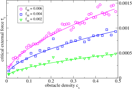
In Fig. 7 and Fig. 8, the theoretical predictions are compared to simulations data. It is worth noticing that the critical force variation against density corresponds to a more convex curve than for shorter cutoff $w\leq 0.5$. An analysis in term of power law fit leads to an exponent smaller than unity. For instance in Fig. 7, for $L_{y}=500$ and $L_{x}=1000$, the effective density exponent is around $\alpha=0.65$. The effective density exponent of $\tau_{c}$ is found to decrease when $w$ increases (see further Sec. 3.3). In Fig. 7, the computations have been performed for different aspect ratios of the lattice and show the same trend as in Fig. 4 for a shorter $w$, the critical force density exponent increases with $L_{x}$ and decreases with $L_{y}$. Although a satisfactory agreement is obtained for the different lattices, we notice that the pinning force $f_{M}$ is smaller than in Fig. 4. Actually the field of validity for the VSC theory is narrower for $w=1$ than for $w<0.5$. The limit of application for the theory decreases as the interaction cutoff increases. Such a limit also varies with the lattice dimensions: it decreases when $L_{y}$ increases and when $L_{x}$ decreases. For instance, with $L_{y}=200$ and $L_{x}=1500$, the theory proves to be efficient as seen from Fig. 8 where the comparison has been performed for different pinning forces the maximum of which is $f_{M}=0.006$. The same computations carried out for $L_{y}=2000$ and $L_{x}=500$, keeping constant both $w$ and $f_{M}$ yield much worse results, in particular for the low densities. This can be understood comparing the critical profiles for both geometries. Whereas the chain profile is quasi-straight for the former the critical profile is wavy for the latter, i.e., similar to the one seen in Fig. 1. As for short cutoffs, the system undergoes a bifurcation passing from a quasi-straight critical profile to a wandering one. The change in critical profile occurs for smaller $f_{M}$ with $w=1$ than for $w<0.5$.

3.3 Extension to intermediary and still broader cutoffs

In previous computations, we developed the pinning force function as a Taylor series around $x_{\infty}$, i.e., the asymptotic solution for the chain nodes position. For intermediary cutoff, namely $0.5<w<1$, we must be aware that such a development cannot be used to approach the non-analytic force function since the cutoff occurs right in between two rows. Then $x_{\infty}$ is assumed to remain far from the cutoff interaction with the next nearest row. The asymptotic position $x_{\infty}$ is thus given by Eq. 12 and $\alpha$ by Eq. 13. The top of the bulge is assumed to be situated above the cutoff distance from the next nearest row. Then the equation on $x_{0}$ is same as in Sec. 3.2 and can be solved analytically as shown in Eq. 28. The equation relating $\tau$ to $\epsilon_{0}$ must be rederived. The sum of the equations in Eq. 20 from rank 1 to rank p, taken sufficiently large, leads to an equation which the linear order in p is now:

$$\tau=-g(x_{0})-\frac{1}{[n-m/2]}\big{[} \epsilon_{0}\frac{f^{\prime}(x_{\infty})}{1-e^{-\alpha}}+\epsilon_{0}^{2}\frac{f^{\prime\prime}(x_{\infty})}{2(1-e^{-2\alpha})}+\epsilon_{0}^{3}\frac{f^{\prime\prime\prime}(x_{\infty})}{6(1-e^{-3\alpha})}$$ (34)

$$+ \sum_{j<l_{b}}g(x_{n+jm})\big{]},$$

where $l_{b}$ is such as $(x_{n+l_{b}m}>1-w)$. The quantity $l_{b}$ corresponds to the segment of the bulge which overpasses the interaction cutoff with next nearest row. Such equation for $\tau$ holds provided that $l_{b}$ remains small compared to $L_{y}/m$.

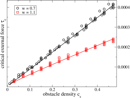
In Fig. 9, the predictions from the present development are compared to simulations data for $w=0.7$. We reported the results obtained from simulations with different obstacle densities. For some densities, we carried out the simulations with different random distributions. The simulations data are distributed around the theoretical predictions which confirms the robustness of the theory.

Figure 9: (color online) External force required to drag a spring chain of length $L_{y}=1000$ over a distance $L_{x}=200$, for a pinning strength $f_{M}=0.001$ and different interaction range $w$ (see legend). The different symbols represent the simulations data and the continuous lines correspond to the prediction made through the theory detailed in the text.

The previous computations can also be extended to an interaction cutoff larger than the unit cell parameter (i.e., $w>1$). In the theory, the function $g(x_{j})=c_{v}f(x_{j}-1)$ is substituted with $g(x_{j})=c_{v}f(x_{j}-1)+h(x_{j})$ where $h(x_{j})=c_{s}f(x_{j}-2)$ accounts for the pinning force due to the still further row, i.e., the second next nearest one. The top of the bulge may interact with such a row meanwhile the back of the chain is assumed to remain far from it. Then the equations found in Sec. 3.2 for $x_{\infty}$ and $\alpha$ still hold and $x_{0}$ is again given by Eq. 27 but substituting the function $g(x)$ with the expression $g(x_{j})=c_{v}f(x_{j}-1)+h(x_{j})$. The equation on $\tau$ follows:

$$\tau=-g(x_{0})+\frac{1}{[n-\frac{m}{2}]}\big{[} \frac{(m+1)^{2}}{8m}g(x_{\infty})-\epsilon_{0}\frac{(f^{\prime}(x_{\infty})+mg^{\prime}(x_{\infty}))}{1-e^{-\alpha}}$$ (35)

$$-\epsilon_{0}^{2}\frac{(f^{\prime\prime}(x_{\infty})+mg^{\prime\prime}(x_{\infty}))}{2(1-e^{-2\alpha})}$$

$$-\epsilon_{0}^{3}\frac{(f^{\prime\prime\prime}(x_{\infty})+mg^{\prime\prime\prime}(x_{\infty}))}{6(1-e^{-3\alpha})}+\sum_{j<l_{b}}h(x_{n+jm})\big{]},$$

where $l_{b}$ corresponds to the top of the bulge overpassing the distance cutoff with the second next nearest row, defined as $(x_{n+l_{b}m}>2-w)$. In Fig. 9, the theoretical computation for $\tau_{c}$ against the obstacle density is compared with simulation data for $(w=1.1)$ and for different random distributions. Although the theory could certainly be improved by accounting for the effect of the nearest row at the back of the chain, the agreement with simulations data proves quantitative.

The results obtained in both cases, $w=0.7$ and $w=1.1$ show that $\tau_{c}$ decreases with $w$. This was confirmed by other simulations performed for still larger $w$, up to $w=2$. Such a decreases is opposite to the one predicted within the MNL theory for SSH. Moreover according to the MNL theory, the density exponent of $\tau_{c}$ is fixed to $\eta=2/3$, whereas according to the VSC sampling theory such an exponent depends on lattice dimensions (see Sec. 3.2) and $w$, as well. For instance, in Fig. 9, a power law fit on the theoretical predictions yields and effective exponent $\eta=0.945$ for $w=0.7$ while for $w=1.1$ we obtained $\eta=0.827$. The variations $\eta$ with lattice dimensions, along with its value larger than $2/3$ and its $w$ dependence demonstrate that the MNL theory does not apply to the systems studied here. The same conclusion holds for other SSH theories predicting a constant density exponent of the critical depinning threshold.

4 Summary and perspectives

In the present study, we addressed a discrete version of a paradigmatic problem, namely the depinning threshold of an elastic string on a random substrate. For a planar distribution of weak pinning points, a theory was devised to compute the applied force required to drag the one-dimensional elastic manyfold over a disordered potential landscape with various aspect ratios. The theoretical predictions were found accurate provided the critical configuration remains close from a quasi-straight line bounded between two lattice rows. The strongest pinning configuration was shown to hinge on the denser lattice rows in which the largest vacant site clusters (VSC) are bounded in size. Such maximum VSC correspond to the weakest lattice defects on which the critical depinning proceeds. The mean size of the critical VSC is determined through an expression involving only lattice dimensions and the overall planar obstacle density $c_{s}$. The theory allowed us to account for the finite lattice size effects in a quantitative manner. The typical variations of the critical applied force against the chain length and the drag distance both yield a logarithmic power law. For a fixed lattice geometry, and an interaction cutoff inferior to half the lattice cell parameter the pinning strength was found close to being linear in $c_{s}$. The effective density exponent $\eta$ of the depinning threshold was found to depend on the lattice geometry and to decrease as the interaction cutoff $w$ increases.

In some atomistic studies bearing on dislocation in a model Ni(Al) solid solution, i.e., with a rather marked size effect[28], the maximum force exerted by isolated solute atoms on a dislocation segment was found of the order of $0.04$ nano-Newton (nN). The elastic contribution to the line tension of a screw dislocation, computed within the isotropic elastic theory [37] is $\Gamma=\Gamma_{S}\ln(R/b)$ where $b$ is the Burgers vector, $R$ is the inter-dislocation spacing and where the pre-logarithmic factor is given by $\Gamma_{S}=\mu b^{2}(1+\nu)/4\pi(1-\nu)$, with $\mu$ as the shear modulus and $\nu$ as the Poisson coefficient. The distance $R$ is related to the dislocation density $\rho_{d}$ by $R=1/\sqrt{\rho_{d}}$ which for a standard density in deformed metals $\rho_{d}=10^{12}$ m^-2, gives $R=1$ $\mu$m. Then, with $\mu_{Ni}=74600$ MPa and $\nu=0.28$, the screw dislocation line tension in Ni is $\Gamma=6.1$ nN which gives a ratio between the obstacle pinning strength and the line tension of $f_{M}=0.007$, of the order of $f_{M}$ studied in the present work. A solute atom dilation smaller than the one for Al in a Ni matrix or a smaller dislocation density could even yield smaller $f_{M}$. In regard of the simplicity of the elastic manyfold model, the present study requires to be extended to a more realistic model involving some of the atomistic details as for instance: (i) a position dependant obstacle strength, (ii) a dissociated core, and (iii) mixing of different types of obstacles. Such extensions would allow to address longstanding issues in SSH theory.

References

- [1] N. Mott, Imperfections in Nearly Perfect Crystals, John Wiley, New York, 1952, p.173.
- [2] N. Mott, F. Nabarro, Report on the Strength of Solids, Physical Society, London, 1948, pp. 1-19.
- [3] F. Nabarro, Dislocations and Properties of Real Materials, The Institute of Metals, London, 1985, p. 152.
- [4] J. Friedel, Dislocations, Addison-Wesley, New York, 1964, p. 224.
- [5] R. Labusch, Acta Metall. 20 (1972) 917.
- [6] R. Fleischer, Acta Metall. 11 (1963) 203.
- [7] R. Fleischer, The Strengthening of Metals, Reinold Press Edition, 1964, p. 93.
- [8] R. Fleischer, W. Hibbard, The relation between Structure and Mechanical Properties of Metals, Vol. 1, H.M.S.O., London, 1963, p. 262.
- [9] T. Suzuki, S. Takeuchi, H. Yoshinaga, Dislocation Dynamics and Plasticity, Springer-Verlag, Berlin Heidelberg, 1991, p. 32.
- [10] S. Zapperi, P. Ciseau, G. Durin, E. Stanley, Phys. Rev. B 58 (1998) 6353.
- [11] J. Joanny, P. de Gennes, J. Chem. Phys. 81 (1984) 552.
- [12] G. Blatter, M. Feigelman, V. Geshkenbein, A. Larkin, V. Vinokur, Rev. Mod. Phys. 66 (1994) 1125.
- [13] S. Brazovskii, T. Nattermann, Adv. Phys. 53 (2004) 177.
- [14] J. Kierfeld, V. Vinokur, Phys. Rev. Lett. 96 (2006) 175502.
- [15] E. Bouchaud, J. Phys.: Condens. Matter 9 (1997) 4319.
- [16] D. Fisher, Phys. Rev. Lett. 56 (1986) 1964.
- [17] O. Narayan, D. Fisher, Phys. Rev. B 48 (1993) 7030.
- [18] P. Chauve, T. Giamarchi, P. LeDoussal, Phys. Rev. B 62 (2000) 6241.
- [19] K. Wiese, Acta Physica Slovaca 52 (2002) 341.
- [20] A. Tanguy, T. Vettorel, Eur. Phys. J. B 38 (2004) 71.
- [21] Y. M. Blanter, V. Vinokur, Phys. Rev. B 66 (2002) 132101.
- [22] A. Rosso, P. LeDoussal, K. Wiese, Phys. Rev. B 75 (2007) 220201.
- [23] E. Rodary, D. Rodney, L. Proville, Y. Bréchet, G. Martin, Phys. Rev. B 70 (2004) 054111.
- [24] D. Olmsted, L. Hector, W. Curtin, R. Clifton, Model. Simul. Mater. Sci. Eng. 13 (2005) 371.
- [25] L. Proville, D. Rodney, Y. Bréchet, G. Martin, Phil. Mag. 86 (2006) 3893.
- [26] K. Tapasa, D. Bacon, Y. N. Osetsky, Model. Simul. Mater. Sci. Eng. 14 (2006) 1153.
- [27] K. Tapasa, D. Bacon, Y. N. Osetsky, Acta Mater. 55 (2007) 93.
- [28] S. Patinet, L. Proville, Phys. Rev. B 78 (2008) 104109.
- [29] J. Marian, A. Caro, Phys. Rev. B 74 (2006) 024113.
- [30] W. Curtin, D. Olmsted, L. Hector, Nature Materials 5 (2006) 875.
- [31] R. Madec, B. Devincre, L. Kubin, T. Hoc, D. Rodney, Science 301 (2003) 1879.
- [32] A. Foreman, M. Makin, Phil. Mag. 14 (1966) 911.
- [33] T. Nogaret, D. Rodney, Phys. Rev. B 74 (2006) 134110.
- [34] Z. Xu, R. Picu, Phys. Rev. B 76 (2007) 94112.
- [35] M. Hiratani, V. Bulatov, Phil. Mag. Lett. 84 (2004) 461.
- [36] R. Arsenault, D. Esterling, Metallurgical Transactions A 20 (1989) 1411.
- [37] J. Hirth, J. Lothe, Theory of dislocations, Wiley Interscience, New York, 1982, p. 180.