Skyrmion vibrational energies with a generalized mass term

Abstract

We study various properties of a one parameter mass term for the Skyrme model, originating from the works of Kopeliovich, Piette and Zakrzewski KPZ , through the use of axially symmetric solutions obtained numerically by simulated-annealing. These solutions allow us to observe asymptotic behaviors of the $B=2$ binding energies that differ to those previously obtained PZ . We also decipher the characteristics of three distinct vibrational modes that appear as eigenstates of the vibrational Hamiltonian. This analysis further examine the assertion that the one parameter mass term offers a better account of baryonic matter than the traditional mass term.

I Introduction

Being one of the primary candidates for an effective low-energy theory of QCD, the Skyrme model Skyrme1 ; Skyrme2 ; Skyrme3 ; Skyrme4 has relished from a large amount of study after which it was realized that it possessed the same symmetry properties as QCD in the limit of large $N_{c}$ Witten1 . The topological solitons that appear as solutions to the model’s equations of motion are identified as mathematical representations of nuclear matter. These solitons, or Skyrmions, are then quantized to obtain physical properties of nuclei. Studies have shown that for the nucleon $B=1$, these calculated properties are within a 30% margin of error from experimental data Adkins1 .

However, when one raises the baryonic number to any $B\geq 2$, the solutions that have been obtained thus far do not correctly describe the presumed geometric properties of nuclear matter. Experimental data indicates that the nucleons seem to preserve their individuality within nuclei. For example, the $B=2$ solutions have the geometrical shape of a toroid, whereas the deuteron, the only stable nuclei with $B=2$, has the presumed shape of two deformed nucleons lightly bound together. Another problem is that the binding energy of the toroidal Skyrmion is much too high, roughly $\sim 80$ MeV (Recall that the deuteron has a binding energy of 2.224 MeV), which is also a likely contributing factor to the odd toroidal shape it possesses. Even worst, both the geometrical shape and binding energy problems persist and are amplified as we increase the value of $B$. For these reasons, the solitonic field configurations within the standard Skyrme model can be viewed as too malleable in the sense that Skyrmions deform noticeably as they form a bound state. For the purpose of comparison here we shall use vibrational energies as a quantifiable measure of rigidity (as opposed to malleability) of the field and analyze the ratio $\frac{\omega_{i}}{E^{tot}}$, where $i=br,2,3$ labels the vibrational energy of the breathing mode and the two other eigenmodes, and where $E^{tot}$ is the total energy of the soliton (more on this in Sec. III). Reaching for higher rigidity solutions can also be understood intuitively by the fact that every nucleon within a nuclei of $B=2$ or higher should presumably be deformed while maintaining its individuality within the nucleus, and not meld with others to form complex geometrical objects. A pragmatic goal towards improving the model would be to find extensions to the current model that point toward a solution to these issues. Therefore, in this optic, one may consider various generalizations of the original Skyrme Lagrangian to find which types lowers the binding energies. In this paper, we limit our analysis to a one-parameter generalization to the standard mass term of the Skyrme model.

In the following, we begin by reviewing the standard Skyrme model as well as reveal the studied generalized mass term that introduces a dimensionless parameter labeled $D$. Initially considered and analyzed by Piette and Zakrewski PZ , this new mass term is studied further in the context of rigidity here using the simulated-annealing numerical algorithm to accurately and effectively minimize the pion field configuration. These exact solutions allow us to deepen our understanding of the dependency between binding energies and the parameter $D$, and will also enable us to conclude that solitonic solutions obtained through the rational map ansatz PZ are not good indicators of this dependence (Sec. IV). We consider solutions for $B=1$ and $B=2$ with axially symmetric configurations. For $B=1$, axial symmetry is an exact symmetry both for the static solution and the rotationally deformed solution. Both calculation will be performed providing a quantitative insight on such deformations otherwise shown to be significant Battye:2005 ; Magee ; Marleau2 . For $B=2,$ the situation is somewhat different. Rotational deformation breaks axial symmetry and would in principle require a full 3D computation. So only the static energy will be minimized for the $B=2$ case even though axially symmetric solutions were found to be a good approximation in Marleau2 . This was done in order to make the numerical efforts more tractable and time efficient. Furthermore, the same solutions are used to compute how the vibrational energies of three eigenstates behave as we increase $D$. The methods used for this analysis is outlined in Sec. III, and the results indicate quantitatively that the mass term increases the rigidity of Skyrmions with $B=1$ while its effect on the binding energy depend on (iso-)spin.

II The Skyrme model with an extended mass term

The model initially proposed by Skyrme comprised of the two term Lagrangian

$$L=\int d^{3}x\left[-\frac{F_{\pi}^{2}}{16}\,Tr\left(L_{\mu}L^{\mu}\right)+\frac{1}{32e^{2}}\,Tr\left([L_{\mu},L_{\nu}]^{2}\right)\right],$$ (1)

where $L_{\mu}=U^{{\dagger}}\partial_{\mu}U$ are the chiral currents associated to the three component pion fields $\mathbf{\pi}$ such that the $SU(2)$ matrix $U$ is defined by

$$U=\sigma+i\mathbf{\tau}\cdot\mathbf{\pi}.$$ (2)

$F_{\pi}$ and $e$ are respectively the pion decay constant and the dimensionless Skyrme parameter. The $\mathbf{\tau}$’s found in (2) are simply the Pauli matrices, and the field $\sigma$ is an additional scalar field that must satisfy the constraint $\sigma^{2}+\mathbf{\pi}\cdot\mathbf{\pi}=1$ in order to avoid adding unphysical degrees of freedom and to enable the possibility of having solitonic solutions.

Each solution to (1) with boundary condition

$$U(\mathbf{r},t)\rightarrow 1\quad\text{as}\quad|\mathbf{r}|\rightarrow\infty$$ (3)

fall into distinct topological sectors that are distinguished by their given topological charge, or baryon number. For $B=1$, spherical symmetry can be utilized to extract a convincing picture of a nucleon through the use of the ansatz

$$U=e^{i\tau_{i}\hat{x}_{i}F(r)},$$

where one only has to solve an ordinary differential equation involving the chiral angle $F(r)$ that (1) brings about Adkins1 .

However, the physics that (1) describes lacks in many respects. First, it is possible to add as many higher order terms of the form $Tr\,([L,L]^{n})$ as one wishes, to account for all possible interactions, and it is simply unknown how the sum of such terms would affect the resulting solutions Marleau1 although it is generally assumed that higher order terms in derivatives could be neglected in the low-energy limit. One may also wonder if the two terms of (1), among all the possible terms, are really the two optimal ones for portraying the physics of nuclear matter. Second, all solutions for $B\geq 2$ obtained thus far do not correctly characterize the presumed geometric properties of nuclei that are found in nature. Third, it does not take into account the mass the of pions, but fortunately, this problem is easier to resolve. One can simply add a chiral symmetry breaking term proportional to the pion mass squared, which has first been successfully introduced by Adkins and Nappi Adkins2 , in the form

$$\frac{m_{\pi}^{2}F_{\pi}^{2}}{8}\,Tr\,(\mathbf{1}-U),$$ (4)

where $m_{\pi}$ is the pion mass (We assume that the three pions $\pi^{0}$, $\pi^{+}$, and $\pi^{-}$ are of equal masses). This term has had the added benefit of eliminating shell-like configurations and favoring energy densities that are higher at their centers, which is more appealing since it is known that nucleons have roughly even matter densities within their shell radii. Hence, the Lagrangian (1) together with the mass term (4) is what we consider to be the standard Skyrme model. Of course, as we have mentioned, many additions and modifications can be made, particularly to the mass term (4).

If we only constrain ourselves to mass terms that obey the boundary condition (3), Kopeliovich, Piette and Zakrzewski KPZ have shown that a generalized mass term can have the form

$$\frac{m_{\pi}^{2}F_{\pi}^{2}}{8K}Tr\left(1-\int_{-\infty}^{+\infty}g(p)U^{p}dp\right),$$ (5)

where the function $g(p)$ and constant $K$ must obey

$$\int_{\infty}^{\infty}g(p)dp=1\quad\text{and}\quad K=\int_{\infty}^{\infty}g(p)p^{2}dp.$$ (6)

However, of the many mass terms that are evidently possible, we will study a particular one-parameter family that has the additional property of disfavoring shell-like configurations as did the standard mass term (4). One then hope that this new term might also improve the overall properties of Skyrmions, such as providing a better account of their binding energies. This one-parameter mass term is

$$\frac{m_{\pi}^{2}F_{\pi}^{2}}{8(1-5D)}\,Tr\,(\mathbf{1}-U-D(U^{2}-U^{3})),$$ (7)

is based on the function

$$g(p)=\delta(p-1)+D\,(\delta(p-2)-\delta(p-3))$$

where $K=1-5D$ and the parameter $D$ can span the range $\left[\,0,0.2\,\right[$ . At $D=0.2$, we note that the mass term is infinite.

Following their original proposal of the general term (5), Piette and Zakrzewski PZ studied (7) with the use of rational map (RM) solutions. In Sec. IV, we will show the results of a similar study that use exact numerical solutions instead of approximate RM map solutions. This will demonstrate the limitations of the rational map ansatz when it comes to give a precise measurement of the binding energies as a function of $D$, especially as it approaches the critical value of 0.2.

Before we discuss binding energies, we will describe in the following section how the study of vibrational modes, a worthy study in its own right, can lead us to quantitatively understand how the $B=1$ solutions gradually get more rigid as $D$ increases. The methods used in this paper for calculating the vibrational energies were previously outlined by Hadjuk andt Schwesinger Haj1 , which can be contrasted with the techniques of Barnes et al. Barnes1 and of Lin and Piette LP where the latter performed their vibrational calculations using rational map solutions.

III Vibrational modes and their energies

Originally put forward by Hajduk and Schwesinger Haj1 , the method for obtaining the vibrational modes and their energies begins by performing the global scale transformation

$$\sigma(x)\rightarrow\sigma(\beta_{k}x_{k})\quad\text{and}\quad\pi_{a}(x)\rightarrow\pi_{a}(\beta_{k}x_{k}),$$ (8)

where the $\beta_{k}$ are scaling parameters, and where we have assumed that the scaling is uniform with respect to the Cartesian coordinates $x$, $y$ and $z$. The advantage of such a scaling lies in its simplicity both in its mathematical and numerical treatment. Its disadvantage is that it is certainly not as general as would be an arbitrary local scale transformation. However, it allows to compute vibrational modes that probe the global rigidity of Skyrmions, giving us a clearer indication whether or not (and how) the field configurations are getting more rigid with respect to the parameter $D$. Substituting (8) into (1) together with the new mass term (7) yields a Lagrangian of the form

$$L=\frac{1}{2}M_{ij}(\beta)\frac{\dot{\beta_{i}}\dot{\beta_{j}}}{\beta_{i}\beta_{j}}-V(\beta),$$ (9)

where the matrices $M_{ij}(\beta)$ and $V(\beta)$ are obtained by direct inspection after all substitutions are made. Since we are only concerned with small amplitude oscillations, we perform an expansion around the minimum of $V$ by taking

$$\beta_{i} =\beta^{0}_{i}e^{\eta_{i}}=\beta^{0}_{i}(1+\eta_{i}+\frac{1}{2}\eta^{2}_{i}+...)$$ (10)

$$\dot{\beta_{i}} =\beta^{0}_{i}\dot{\eta_{i}},$$ (11)

which results in the expansion of $M_{ij}$ and $V$ as

$$M_{ij}(\beta) =M_{ij}\Big{|}_{\beta^{0}_{1},\,\beta^{0}_{2},\,\beta^{0}_{3}}+\left(\eta_{k}\partial_{k}M_{ij}\right)\Big{|}_{\beta^{0}_{k}}+...$$

$$\approx M^{0}_{ij}+\left(\eta_{k}\partial_{k}M_{ij}\right)\Big{|}_{\beta^{0}_{k}}$$ (12)

$$V(\beta) =V\Big{|}_{\beta^{0}_{1},\,\beta^{0}_{2},\,\beta^{0}_{3}}+\frac{1}{2}\eta_{i}\eta_{j}(\partial_{i}\partial_{j}V)\Big{|}_{\beta^{0}_{1},\,\beta^{0}_{2},\,\beta^{0}_{3}}+...$$

$$\approx V^{0}+\frac{1}{2}\eta_{i}\eta_{j}v_{ij}.$$ (13)

Keeping only terms up to order $O(\eta^{2})$ gives us the Lagrangian

$$L=\frac{1}{2}M^{0}_{ij}(\beta)\dot{\eta_{i}}\dot{\eta_{j}}-\frac{1}{2}\eta_{i}\eta_{j}v_{ij}.$$ (14)

In order to compute the vibrational Hamiltonian we must now find a coordinate transformation that satisfies

$$A^{T}M^{0}A=1,$$ (15)

where $\eta=A\xi$. When such a transformation is found, it gives

$$L=\frac{1}{2}\dot{\xi_{i}}\dot{\xi_{j}}-\frac{1}{2}(A^{T}vA)_{ij}\xi_{i}\xi_{j},$$ (16)

which can simply be turned into the Hamiltonian

$$H_{vib}=\frac{1}{2}\sum_{i}\frac{\partial^{2}}{\partial\xi^{2}_{i}}+\frac{1}{2}\left(A^{T}vA\right)_{ij}\xi_{i}\xi_{j}.$$ (17)

We now need to diagonalize the matrix $(A^{T}vA)_{ij}$ in order to obtain the vibrational eigenstates and eigenvalues. Thus, we need to solve the eigenvalue equation

$$\left(B^{T}A^{T}vAB\right)_{ij}=\omega^{2}_{i}\delta_{ij},$$ (18)

where the matrix $B$ must satisfy $B^{T}B=1$. The energies associated to the eigenstates $B_{1j}$, $B_{2j}$, et $B_{3j}$ are then

$$E_{i}^{vib}=\left(n_{i}+\frac{1}{2}\right)h\omega_{i}.$$ (19)

However, in our study, we set the zero-point energy to zero, in other words we set

$$E_{i}^{vib}=hn_{i}\omega_{i}$$ (20)

because the zero-point energy of vibrational modes is ill-defined. This is procedurally how we obtained our eigenstates (eigen-modes) and eigenvalues (eigen-energies) from our numerical solutions. But, before we discuss the results of our vibrational analysis of $B=1$ solitons, we must briefly describe what exactly are the numerical solutions we are working with. For simplicity, we shall from hereon identify vibrational frequencies $\omega_{i}$ as vibrational energies although they are not exactly the same (see eqn. (19)).

Beginning from the Lagrangian (1), we added the mass term (7), yielding the static energy

$$E_{s}^{B} =\int d^{3}x\left[-\frac{F_{\pi}^{2}}{16}\,Tr\left(L_{i}L^{i}\right)+\frac{1}{32e^{2}}\,Tr\left([L_{i},L_{j}]^{2}\right)\right]$$

$$+\frac{m_{\pi}^{2}F_{\pi}^{2}}{8(1-5D)}\,Tr\,(\mathbf{1}-U-D(U^{2}-U^{3})),$$ (21)

where $i$ and $j$ run over spatial components only and $B$ is the baryonic number. The minimal energy Skyrmion for $B=1$ and $B=2$ turns out to have spherical and axial symmetry respectively. Since we are only interested by these values of $B$, the general solution will be cast in the form of the axial ansatz

$$\sigma=\psi_{3}\hskip 28.45274pt\pi_{1}=\psi_{1}\cos n\theta\hskip 28.45274pt\pi_{2}=\psi_{1}\sin n\theta\hskip 28.45274pt\pi_{3}=\psi_{2}$$ (22)

introduced in Krusch:2004uf where $\boldsymbol{\psi}(\rho,z)=(\psi_{1},\psi_{2},\psi_{3})$ is a three-component unit vector that is independent of $\theta$. The boundary conditions at infinity implies that $\boldsymbol{\psi}\rightarrow\left(0,0,1\right)$ as $\rho^{2}+z^{2}\rightarrow\infty$. Moreover, we must impose that $\psi_{1}=0$ and $\partial_{\rho}\psi_{2}=\partial_{\rho}\psi_{3}=0$ at $\rho=0$.

With the axial ansatz (22), we can also set the scaling length and energy in units of ${2\sqrt{2}}/{eF_{\pi}}$ and ${F_{\pi}}/{2\sqrt{2}}$ respectively, giving expressions for the static energy and the baryon number that read

$$E_{s}^{B} =-\int\text{d}^{3}x\mathcal{L}_{S}$$

$$=2\pi\left(\frac{F_{\pi}}{2\sqrt{2}e}\right)\int\text{d}z\text{d}\rho\rho\biggl{\{}\left(\partial_{\rho}\boldsymbol{\psi}\cdot\partial_{\rho}\boldsymbol{\psi}+\partial_{z}\boldsymbol{\psi}\cdot\partial_{z}\boldsymbol{\psi}\right)\left(1+n^{2}\frac{\psi_{1}^{2}}{2\rho^{2}}\right)$$

$$+\frac{1}{2}|\partial_{z}\boldsymbol{\psi}\times\partial_{\rho}\boldsymbol{\psi}|^{2}+n^{2}\frac{\psi_{1}^{2}}{\rho^{2}}+\frac{2\beta^{2}}{(1-5D)}\left(1-\psi_{3}\right)\left(1+D\left(1-2\psi_{3}-4\psi_{3}^{2}\right)\right)\biggr{\}}$$ (23)

$$B=\frac{n}{\pi}\int\text{d}z\text{d}\rho\,\psi_{1}|\partial_{\rho}\boldsymbol{\psi}\times\partial_{z}\boldsymbol{\psi}|$$ (24)

with $\beta=\frac{2\sqrt{2}m_{\pi}}{eF_{\pi}}$.

Also, for all our minimizations, we fixed the constants $F_{\pi}$, $e$, and $m_{\pi}$ to

$$F_{\pi}=129\,\text{MeV},\quad e=5.44\,\text{MeV}^{-1},\quad\text{and}\quad m_{\pi}=138\,\text{MeV}.$$

The values of $F_{\pi}$ and $e$ were set according to ref. KPZ for comparative purposes. At such values, the Skyrme model reproduces the mass of the nucleon and of the delta when one discounts the mass term Adkins1 . Regarding the mass term, $m_{\pi}$ is set to its experimental value and the parameter $D$ varies in order to probe how the mass term in (21) might affect the Skyrmion’s properties. Of course, when the mass term is switched on, the prediction for the nucleon and delta masses will deviate from their experimental values. This could be corrected with an appropriate choice of $F_{\pi}$ and $e$, however here we shall retain $F_{\pi}=129$ MeV and $e=5.44$ MeV^-1, since we are more interested in certain ratios of energies than in the actual values of energies, and comparisons with earlier works are easier.

Physical states such as the nucleon and the deuteron require an additional contribution to the energy, the rotational and isorotational energy due to spin and isospin of these states. For the nucleon, this is done by fixing the quantum numbers of spin and isospin to $I=J=\frac{1}{2}$, and assuming axial symmetry, it leads to the total isorotational and rotational energy of the form

$$E_{rot}^{1}=\frac{1}{4}\left[\frac{\left(1-\frac{W_{11}}{U_{11}}\right)^{2}}{V_{11}-\frac{W_{11}^{2}}{U_{11}}}+\frac{1}{U_{11}}+\frac{1}{2U_{33}}\right].$$ (25)

Similarly for the deuteron one gets

$$E_{rot}^{2}=\frac{1}{V_{11}}.$$ (26)

Here $U_{11}$, $U_{33}$, $V_{11}$, and $W_{11}$ are moments of inertia which follows the definition in the works of Houghton and Magee Magee and Fortier and Marleau Marleau2 . Accordingly the components of these inertia tensors are

$$U_{11} =2\pi\left(\frac{2\sqrt{2}}{e^{3}F_{\pi}}\right)\int\text{d}z\text{d}\rho\rho\biggl{\{}\psi_{1}^{2}+2\psi_{2}^{2}+\frac{1}{2}\biggl{[}\left(\partial_{\rho}\boldsymbol{\psi}\cdot\partial_{\rho}\boldsymbol{\psi}+\partial_{z}\boldsymbol{\psi}\cdot\partial_{z}\boldsymbol{\psi}+n^{2}\frac{\psi_{1}^{2}}{\rho^{2}}\right)\psi_{2}^{2}$$ (27)

$$+\left(\partial_{\rho}\psi_{3}\right)^{2}+\left(\partial_{z}\psi_{3}\right)^{2}+n^{2}\frac{\psi_{1}^{4}}{\rho^{2}}\biggr{]}\biggr{\}},$$ (28)

$$U_{33} =2\pi\left(\frac{2\sqrt{2}}{e^{3}F_{\pi}}\right)\int\text{d}z\text{d}\rho\rho\psi_{1}^{2}\left(\partial_{\rho}\boldsymbol{\psi}\cdot\partial_{\rho}\boldsymbol{\psi}+\partial_{z}\boldsymbol{\psi}\cdot\partial_{z}\boldsymbol{\psi}+2\right),$$ (29)

$$V_{11} =2\pi\left(\frac{2\sqrt{2}}{e^{3}F_{\pi}}\right)\int\text{d}z\text{d}\rho\rho\biggl{\{}|\rho\partial_{z}\boldsymbol{\psi}-z\partial_{\rho}\boldsymbol{\psi}|^{2}\left(1+n^{2}\frac{\psi_{1}^{2}}{2\rho^{2}}\right)+z^{2}n^{2}\frac{\psi_{1}^{2}}{\rho^{2}}+\frac{1}{2}\left(\rho^{2}+z^{2}\right)|\partial_{\rho}\boldsymbol{\psi}\times\partial_{z}\boldsymbol{\psi}|^{2}\biggr{\}},$$ (30)

$$W_{11} =2\pi\left(\frac{2\sqrt{2}}{e^{3}F_{\pi}}\right)\int\text{d}z\text{d}\rho\rho\biggl{\{}\left[\psi_{1}\left(\rho\partial_{z}\psi_{2}-z\partial_{\rho}\psi_{2}\right)-\psi_{2}\left(\rho\partial_{z}\psi_{1}-z\partial_{\rho}\psi_{1}\right)\right]\biggl{(}1+\frac{1}{2}\left[\left(\partial_{z}\psi_{3}\right)^{2}+\left(\partial_{\rho}\psi_{3}\right)^{2}+\frac{\psi_{1}^{2}}{\rho^{2}}\right]\biggr{)}$$ (31)

$$\phantom{=2\pi\left(\frac{2\sqrt{2}}{e^{3}F_{\pi}}\right)\int\text{d}z\text{d}\rho\rho\biggl{\{}}+\frac{\psi_{3}}{2}\left(z\partial_{z}\psi_{3}+\rho\partial_{\rho}\psi_{3}\right)\left[\partial_{\rho}\psi_{2}\partial_{z}\psi_{1}-\partial_{\rho}\psi_{1}\partial_{z}\psi_{2}\right]+\frac{z\psi_{1}\psi_{2}}{2\rho}\left(2+\partial_{\rho}\boldsymbol{\psi}\cdot\partial_{\rho}\boldsymbol{\psi}+\partial_{z}\boldsymbol{\psi}\cdot\partial_{z}\boldsymbol{\psi}\right)\biggr{\}}.$$ (32)

Finally, the nucleon and deuteron mass are the sum of the appropriate static and rotational energies $E_{B}^{s}+E_{B}^{rot}$ with $B=1,2$ respectively.

Having fixed the model’s parameters, we then used the algorithms of simulated-annealing to accomplish the minimization of (21) for values of $D$ ranging from 0 to 0.1999. As examples of one of our minimizations, the energy density of the $B=1,2$ Skyrmions for values of the parameter $D=0$ and $D=0.195$ are shown in Figure 1.

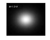
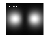
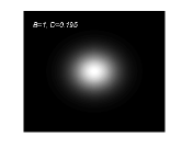
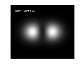
Figure 1: Energy density profiles for $B=1$ and $B=2$ and for values of parameter $D=0$ and $D=0.195$ (top and bottom line respectively) on the $\rho-z$ plane. Here $\rho$ and $z$ span the region from -1 to 1 in units of ${2\sqrt{2}}/{eF_{\pi}}$.

For each minimization, we used a 250 by 500 point grid, representing the standard cylindrical coordinates $z$ and $\rho$ respectively, which provides sufficient detail for analyzing rotational and vibrational modes. Axial symmetry is therefore implied as it is known to be a symmetry of the $B=1$ hedgehog and $B=2$ toroidal static solutions. These configurations are confirmed by the results in Figure 1 along with the observations that our choice of mass term (7) leads to non shell-like energy densities. As one might have expected from larger mass terms, we also see the size of the Skyrmion decreases as $D$ increases. Once a solution is reached for $B=1$, we compute the matrices $M_{ij}^{0}$ and $v_{ij}$ in equation (14) numerically. We proceed with the appropriate scaling transformation, perform the diagonalization, and finally calculate the eigen-energies of each vibrational mode. By the form of our diagonalization (18), it is clear that we would obtain strictly three eigenvectors depicting three types of vibration for each solution. Strikingly, but comprehensibly, no matter the value of $D$, the three types of vibration obtained were always of the same form.

The first type observed may be identified to the well-known breathing mode described by the eigenvector

$$\frac{1}{\sqrt{3}}(1,1,1)$$ (33)

in Cartesian coordinates. The energy associated to this mode, $\omega_{br}$, along with the total gives a clear picture of how the rigidity of the soliton changes as a function of $D$. Put clearly, the lower the ratio

$$R_{i}=\frac{\omega_{i}}{E_{1}^{s}},\qquad i=br,2,3,$$ (34)

the more the soliton is expected to be deformable, or malleable. In essence, the ratio (34) indicates whether or not the mass term (7) renders a more rigid Skyrmion, which would be desirable for the reasons mentioned earlier. The second type, which we call $\omega_{2}$, can be understood as a vibration along $x$ together with a simultaneous and opposite vibration along $y$, but not $z$. Its eigenvector has the form

$$\frac{1}{\sqrt{2}}(1,-1,0).$$ (35)

The third vibrational type is characterized by a positive vibration along $x$ and $y$, together with a simultaneous opposite vibration along $z$. We call this last type $\omega_{3}$ with eigenvector

$$\frac{1}{\sqrt{6}}(1,1,-2).$$ (36)

These eigenvectors (33), (35), and (36), however, are idealizations of what we actually numerically obtain, even though our numerical approach does come close to this. For example, the three eigenvectors obtained for $D=0.8$ were (neglecting normalization)

$$\left(\begin{array}[c]{c}4.064\\ 4.064\\ 4.093\end{array}\right),\quad\left(\begin{array}[c]{c}4.210\\ -4.210\\ 0\end{array}\right),\,\text{and}\quad\left(\begin{array}[c]{c}2.446\\ 2.446\\ -4.869\end{array}\right).\quad$$

Throughout all our results, an accuracy of this type was the norm.

Table 1 gives the energies of each vibrational mode, together with the static and rotational energies of the $B=1$ soliton. Here the solution was found by minimizing the static energy $E_{s}$.

Table 1: $B=1$ vibrational energies versus $D$ without rotational minimization (MeV)

. $D$ $E_{N}$ $E^{\pi}$ $E_{1}^{rot}$ $E_{1}^{s}$ $\omega_{br}$ $\omega_{2}$ $\omega_{3}$ 0 1011.53 26.67 112.12 899.41 290.08 648.42 646.63 0.02 1014.34 28.14 113.05 901.29 293.47 651.88 649.89 0.04 1017.94 29.85 114.35 903.59 297.78 656.55 654.66 0.06 1021.31 32.51 114.84 906.47 302.15 659.20 657.03 0.08 1026.87 35.38 116.64 910.24 308.67 665.76 663.10 0.1 1034.12 39.31 118.78 915.34 317.59 674.17 671.96 0.12 1044.77 44.65 122.12 922.65 330.16 686.46 684.91 0.14 1061.48 52.51 127.41 934.07 349.54 706.13 704.38 0.16 1091.90 65.36 137.33 954.57 384.15 742.28 740.63 0.18 1164.35 93.18 159.96 1004.39 463.69 824.65 823.08 0.19 1268.19 128.15 191.03 1077.16 573.29 937.29 935.27 0.195 1408.88 170.36 231.13 1177.75 716.27 1082.78 1078.47 0.1975 1591.37 220.0 280.32 1311.05 897.55 1265.10 1261.77 0.199 1907.78 298.78 361.49 1546.30 1194.68 1567.33 1546.77 0.1999 3193.16 578.49 657.96 2535.21 2311.62 2726.74 2660.59

We first note that the energies of the $\omega_{2}$ and $\omega_{3}$ modes are quite similar. Remembering that the only difference between these is a vibration along $z$, we see that this vibration along $z$ diminishes the total energy of the vibration ever so slightly. Furthermore, the energy of the breathing mode rises much faster as a function of $D$ than the other two vibrational modes. Lastly, we notice that the energy of the mass term, $E^{\pi}$, increases significantly with $D$. Yet, even with $D=0.1999$, the mass term represents less than 23% of the total static energy, which is somewhat surprising if we consider the factor $(1-5D)^{-1}$ in front of the mass term. Note that for $D=0.1999$, we still observe a typical hedgehog configuration similar to that of Figure 1 although we are at the frontier $(D=0.2)$ of a breakdown in our numerical procedure. Indeed, the relatively large deviation of $\omega_{2}$ with respect to $\omega_{3}$ for $D=0.1999$ could be an early sign of such a breakdown and caution is advised when interpreting this last set of data.

A second set of computations were performed in parallel to the ones given above by including (iso-)rotational energy in the energy minimization process and therefore allowing for axial deformation of the nucleon. Such effects which have been shown to be significant Battye:2005 ; Magee ; Marleau2 . Thus, adding the (iso-)rotational energy (25) to the static energy (21) and minimizing the nucleon mass instead of the static energy

$$E_{N}=E_{1}^{s}+E_{1}^{rot}$$ (37)

will lead to an axially deformed solution and a new set of data shown in Table 2. We see again that the data for $D=0.1999$ exhibit a rather peculiar behaviour especially regarding the value $\omega_{br}=71.98$. Although there is no obvious signal of a numerical breakdown in the energy and baryon number density configuration, in our opinion the data cannot be trusted. It should be noted that the numerical breakdown is much more drastic for higher values of $D$ where it is generally characterized by scattered densities over the entire grid. The $D=0.1999$ data set is nonetheless listed to illustrate the signature of a possible numerical breakdown.

Table 2: $B=1$ vibrational energies with rotational minimization (MeV)

$D$	$E_{N}$	$E^{\pi}$	$E_{1}^{rot}$	$E_{1}^{s}$	$\omega_{br}$	$\omega_{2}$	$\omega_{3}$
0	990.23	51.52	73.82	916.41	269.61	541.87	540.31
0.02	992.81	53.74	74.19	918.61	274.01	545.53	543.54
0.04	995.98	56.42	74.65	921.33	278.81	549.15	547.23
0.06	999.83	59.94	74.87	924.96	287.45	555.88	553.40
0.08	1004.83	64.24	75.24	929.60	297.15	563.21	560.02
0.1	1011.55	69.77	75.73	935.83	309.24	572.19	568.21
0.12	1020.92	77.35	76.04	944.88	329.01	586.01	579.82
0.14	1035.27	88.27	76.28	958.99	356.36	603.49	595.97
0.16	1060.49	105.10	77.66	982.82	395.82	629.89	616.99
0.18	1118.28	139.27	77.67	1040.61	493.25	680.96	664.99
0.19	1199.51	178.84	79.68	1119.84	603.37	736.22	718.97
0.195	1309.04	224.52	83.31	1225.72	729.46	803.61	783.27
0.1975	1452.83	277.16	89.70	1363.13	808.13	904.12	895.73
0.199	1707.07	360.53	103.82	1603.25	1003.54	1135.50	1043.64
0.1999	2309.34	578.49	151.63	2157.71	71.98	2102.43	1620.67

Notice how little the rotational energy changes with $D$ and how similarly the vibrational energies behave as a function of $D$ with those obtained without rotational term in the minimization. However, there are significant differences between the two sets of data which are best exhibited in a plot of the relevant ratios for both types of minimization. This is shown in Figure 2.

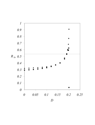
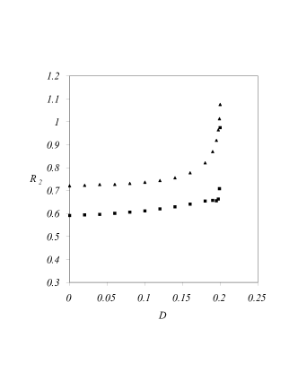
a)                                                         b)

Figure 2: Ratios of vibrational with respect to the static energies $R_{i}=\frac{\omega_{i}}{E_{1}^{s}}$ as a function of the mass parameter $D$ where in a) $i$ labels the vibrational mode $i=br$ and in b) $i=2$. Triangles (squares) correspond to the solutions without (with) rotational energy in the energy minimization. The vertical solid line in a) is the experimental value of ratio $\frac{E_{Roeper}}{E_{N}}$, where $E_{Roeper}$ is the energy of the Roeper resonance, sometimes identified with the breathing mode of the proton, but shown here for comparison purposes only.

The differences between the ratios $\frac{\omega_{i}}{E_{1}^{s}}$ of the minimizations with and without rotational energy are now clear. For the breathing mode, the curves overlap quite well. However, for the other two types of vibration, $\omega_{2}$ and $\omega_{3}$, the added rotational energy to the Lagrangian lowers significantly their energies. Perhaps because $E_{1}^{rot}$ renders a slightly less oblate Skyrmion, the vibrational energies along $\rho$ diminish accordingly. The general tendencies of all curves however indicate that the mass term does add a certain “rigidity” to the field configurations as $D$ increases. What remains to be seen is if there is a correlation between this defined rigidity and the binding energies of $B=2$ solutions. This is done in the next section.

But before analyzing binding energies, we must mention here the complementary results of Lin and Piette LP . The authors consider the vibrational modes of the Skyrme model with the mass term falling into the class of eqs. (5) and (6) namely of the form $Tr(U^{p}-1)$ which differs from (7). They follow the time dependent approach introduced by Barnes et al. Barnes1 to identify the vibrational modes which assumes local instead of global scale transformations that we chose to perform our calculation. Also they use of the rational map ansatz which seems to prevent a precise determination of the vibrational energies. For anyone of these reasons, their results can not be compared directly with ours. Nonetheless they observe a clear increase in the vibrational energies with respect to the mass term which is in qualitative accord with our results.

IV Binding Energies

The results for the static energies of the $B=2$ solitons are presented in Table 3 together with their corresponding binding energies computed from the total static energies of the $B=1$ solitons of Tables 1.

Table 3: $B=2$ energies without rotational minimization (MeV)

$D$		$E_{2}^{s}$	$2E_{1}^{s}-E_{2}^{s}$		$E_{D}$	$2E_{N}-E_{D}$
0		1720.55	78.27		1813.51	209.55
0.02		1724.91	77.66		1818.19	210.49
0.04		1730.18	77.01		1824.65	211.23
0.06		1736.7 8	76.15		1832.75	209.86
0.08		1745.33	75.14		1843.18	210.57
0.1		1756.80	73.88		1857.23	211.00
0.12		1773.14	72.15		1876.94	212.60
0.14		1798.38	69.75		1907.32	215.63
0.16		1843.13	66.02		1961.01	222.79
0.18		1949.56	59.22		2087.19	241.51
0.19		2101.77	52.56		2265.44	270.94
0.195		2308.81	46.69		2505.45	312.32
$0.1975$		$2580.04$	$42.06$		2816.70	366.04
0.199		3054.49	38.10		3355.59	459.97
$0.1999$		$4794.96$	$275.46$		4799.64	1586.68

Also shown are the results for the physical states of deuteron $E_{D}$ versus that of the nucleon $E_{N}$. All results in Table 3 were obtained by minimizing static energies alone, i.e. minimization without rotational energy, to avoid non-axial solutions. We recall here that we have fixed the $F_{\pi}$, $e$ and $m_{\pi}$ parameters of the Skyrme model leading to results for $E_{D}$ and $E_{N}$ that are much higher than their experimental values. While an appropriate fit of the parameters could fix this problem it is not necessary in the context of this work since we are more interested in the relative weight of the vibrational and binding energies than in their actual values. With the data provided by Table 3, we define $R$, the ratio of the energy of the $B=2$ soliton with respect to that of two isolated $B=1$ solitons. $R$ is plotted in Fig. 3 for three sets of points,

$$R=\frac{E_{2}^{s}}{2E_{1}^{s}}$$ (38)

corresponding to (iso-)spinless solitons and

$$R=\frac{E_{D}}{2E_{N}}$$ (39)

for comparison of the deuteron versus two nucleons. These quantities indicates how the relative binding energies change with increasing $D$. The dashed line represents the experimentally measured mass of the deuteron over twice the mass of an individual nucleon ($R=0.9998$).

Clearly, as $D$ approaches its critical value of 0.2, we observe that the binding energies for $I=J=0$ solitons (triangles in Fig. 3) diminish considerably without ever crossing the dashed line or the value $R=1$ which corresponds to the limit of instability of the $B=2$ solution. The sharp increase in $R$ suggest that it may be possible to adjust the value of $D$ such that the relative importance of the binding energy would be arbitrarily small — of course, the solution would still be of toroidal form which is presumably not that of the deuteron. Some cautionary comments are in order here. First the last point for this set of data shows a sharp increase of the binding energy at $D=0.1999$. It is at the boundary of the region of breakdown of our numerical technique and attempts to obtain stable solutions as we push $D$ closer to 0.2 were not successful. Also the limit $D\rightarrow 0.2$ is ill-defined and approaching this limit is physically questionable as the contributions of the mass term which breaks the $SU(2)$ symmetry gets relatively large.

Surprisingly, the situation is more obscure for the deuteron-nucleon data. A first set of data, based on static energy minimization (squares in Fig. 3), shows that the relative importance of the binding energy is quite insensitive to $D$ up to $0.17$ but increases (i.e. $R$ decreases) dramatically as $D$ approaches the critical value of $0.2$ contrarily to what is observed for the spinless Skyrmion. This is entirely due to the distinct behavior of the $B=2$ and $B=1$ rotational energies. Of course rotational deformations may affect this behaviour. To provide some measure of that effect we present a third set of points on Fig. 3 (circles) where $R$ is computed with the $B=2$ static and $B=1$ rotationally deformed solutions. Note that an exact full 3D $B=2$ rotationally deformed computation would lower $R,$ and so this third set of data represent the absolute maximum of $R$ for the deuteron-nucleon system. Again the mass term (7) that we analyzed always lead to bound states ($R<1$) which is an interesting result by itself. However the observation of this opposite behavior with respect to the parameter $D$ for these last two sets of data emphasizes the importance of the rotational deformations. It may well be that a full 3D computation of $B=2$ deformed solution leads to a behaviour closer to that of the second set of data (squares) but our results does not allow to infer on the exact nature of the bound state for the deuteron. Perhaps a full 3D computation allowing for non-axial deformation of the deuteron would conclude otherwise. It is also clear that the bound states of spinless Sakyrmions and deuteron-nucleon system may show completely different behaviour.

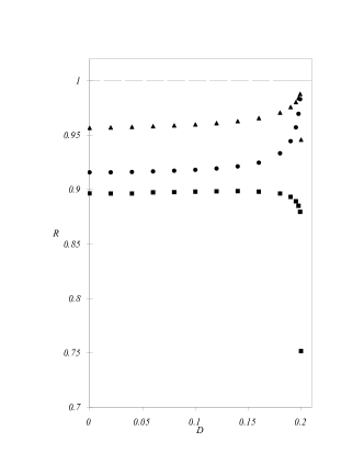
Figure 3: Ratios $\frac{E_{2}^{s}}{2E_{1}^{s}}$ (triangles) and $\frac{E_{D}}{2E_{N}}$ (squares) as a function of the mass parameter $D$. The dashed line at $R=1$ corresponds to the limit of instability of the bound state whereas the experimental value for $\frac{E_{D}}{2E_{N}}=0.99979$, i.e. very close to 1.

Additionally, these results put into question the conclusions obtained by Piette and Zakrzewski PZ . Their results show that for a $D$ larger than approximately 0.12, the toroidal configuration is an unstable one because its total energy is larger than twice that of a single nucleon. More precisely, their results indicate that the ratio $\frac{E_{2}^{s}}{2E_{1}^{s}}$ crosses 1 at $D\approx 0.12$ and continues to increase afterwards, in contradiction with our results (Fig. 3). This discrepancy suggests that the use of the rational map ansatz does not adequately minimize the energies of the $B=2$ configurations, and that we cannot have too much confidence in its ability to truly find the minimal solutions of any $B\geq 2$. Hence, the more exact simulated-annealing approach for finding solutions may be the best way to decipher which model types are more suitable than others. It may also be the only method for finding out why the $B=2$ Skyrmion has a toroidal shape in the first place. There is also certainly a link to make between the increasing rigidity (characterized by $\frac{\omega_{br}}{E_{1}^{s}}$) and the changing binding energy of the solitons as a function of $D$ which also depends on the nature of the solitons, (iso-)spinless or deuteron-nucleons system. In our view, both characteristics are needed for a better model, and hence adds to the appeal of further dynamical or mass terms such as (7).

V Conclusion

From the behaviors of the binding energies (Fig. 3) and the breathing mode energies (Fig. 2a), we can assert that the mass term (7) with a non-zero value of $D$ does not quantitatively succeed in providing a consistent model of nuclear matter in the sense that the experimental value for binding energy of the deuteron was not attainable for the values of $D$ considered here. It also emphasize the need for rotationally deformed $B=2$ computations to determine the exact behaviour as $R$ seems to be very sensitive to rotational deformation near $D=0.2$. Meanwhile it may be premature to conjecture the exact deuteron-nucleon behaviour on the basis of the results for spinless solitons. Our results have also shown that in contrast to the rational map solutions of Piette and Zakrzewski, the behavior of the ratio $\frac{E_{2}^{s}}{2E_{1}^{s}}$ never crosses 1 and seems only to approach 1 in the limit of $D\longrightarrow 0.2$. Hence, this indicates not only that the $B=2$ is a bound state for all values of $D$ considered in this work, but it also demonstrates the clear limitations of the rational map ansatz in providing exact quantitative insight into how the model behaves and works. In conjunction with the behavior of the binding energies, the ratio of $\frac{\omega_{br}}{E_{1}^{s}}$ shows that as $D$ increases the field configurations are more resistant to being vibrationally excited, which is indicative of more rigid solitons and perhaps a relation between rigidity and larger binding energies for the deuteron.

All calculations relied on fixed values for the parameters of the Skyrme model (except for $D$) mostly for comparison purposes with previous work. These parameters are usually fitted to reproduce the experimental values of the mass of the nucleon and delta or other physical quantities. Indeed, the values of the energies we have obtained were sometimes far from those of experimental data. Therefore, some of our conclusions may no longer hold for a more physical choice of Skyrme parameters despite the fact that they were based on the relative importance of each quantity. On the other hand, three dimensional simulated-annealing programs will be needed to explore baryonic numbers beyond 2, and to confirm the validity of axially symmetric solutions for $B=2$. Regarding the prospect of obtaining 2-nucleon shape solitons for $B=2$, it would seem that the mass term in (7) is not sufficient and perhaps we need to rethink what type of lagrangian would permit such a minimal configuration. In any event, it is also possible to add as many parameters in the mass term (7) with higher powers of $U$ as we wish, and this alone may lead us towards a sounder effective theory of QCD.

This work was supported by the National Science and Engineering Research Council of Canada.

References

- (1) T. H. R. Skyrme, Proc. R. Soc. A247, 260 (1958).
- (2) T. H. R. Skyrme, Proc. R. Soc. A260, 127 (1961).
- (3) T. H. R. Skyrme, Proc. R. Soc. A262, 237 (1961).
- (4) T. H. R. Skyrme, Nucl. Phys. 31, 556 (1962).
- (5) E. Witten, Nucl. Phys. B160, 57 (1979).
- (6) G. S. Adkins, C. R. Nappi, et E. Witten, Nucl. Phys. B228, 552 (1983).
- (7) G. S. Adkins, C. R. Nappi, Nucl. Phys. B233, 109 (1984).
- (8) V. B. Kopeliovich, B. Piette and W. J. Zakrzewski, Phys. Rev. D73 014006 (2006).
- (9) B. Piette and W.J. Zakrzewski, Phys. Rev. D77 074009 (2008).
- (10) R. A. Battye, S. Krusch and P. M. Sutcliffe, Phys. Lett.B626, 120 (2005).
- (11) C. Houghton, S. Magee, Phys. Lett. B632, 593-596 (2005).
- (12) J. Fortier and L. Marleau, Phys. Rev. D77 054017 (2008).
- (13) L. Marleau, Can. J. Phys. 73, 6 (1995).
- (14) S. Krusch and P. Sutcliffe, J. Phys. A37 9037 (2004).
- (15) C. Hajduk, and B. Schwesinger, Nucl. Phys. A453, 620 (1986).
- (16) W.T. Lin, and B. Piette, Phys. Rev. D77 125028 (2008).
- (17) C. Barnes, W.K. Baskerville, and N. Turok, Phys. Lett. B411, 180 (1997).