A comparison of local simulations and reduced models of MRI-induced turbulence

Abstract

We run mean-field shearing-box numerical simulations with a temperature-dependent resistivity and compare them to a reduced dynamical model. Our simulations reveal the co-existence of two quasi-steady states, a ‘quiet’ state and an ‘active’ turbulent state, confirming the predictions of the reduced model. The initial conditions determine on which state the simulation ultimately settles. The active state is strongly influenced by the geometry of the computational box and the thermal properties of the gas. Cubic domains support permanent channel flows, bar-shaped domains exhibit eruptive behaviour, and horizontal slabs give rise to infrequent channels. Meanwhile, longer cooling time scales lead to higher saturation amplitudes.

1 Introduction

The observed accretion luminosity of astrophysical disks demands that angular momentum be transported at a rate far in excess of that possible by molecular viscosity in a laminar flow (Shakura & Syunyaev 1973). The magneto-rotational instability (MRI) (Balbus & Hawley 1991) provides a more efficient mechanism: the MRI generates turbulent motions that are strongly correlated and which significantly increase the effective flux of angular momentum. It is hence regarded the most promising candidate responsible for the observed anomalous transport in magnetised disks. Our main observational probes of disks exploit their radiation properties, which in turn strongly depend on their thermal and chemical properties. So in order to connect observations with the dynamical state of accretion disks we must better understand the relationship between MRI turbulence and the chemistry and thermodynamics of accretion disks. The goal of this paper is to make progress to this end.

We shall focus principally on the role of the thermodynamics and in particular, resistive dissipation. From the outset we assume a generic model of radiative loss and fast chemistry, so that the resistivity $\eta$ depends only on temperature. The latter temperature dependence, however, gives rise to an interesting feedback on the turbulent dynamics. Fluctuations in temperature will not only alter the resistive scale, and hence the turbulent cascade of energy (see Fromang et al. 2007; Lesur & Longaretti 2007), it will also influence the linear MRI modes which drive the turbulence itself in regions where the resistivity is sufficiently high.

In order to clarify the intriguing relationship between the disk thermodynamics and the MRI-induced turbulent dynamics, Balbus & Lesaffre (2008) devised a simple 2 variable dynamical system, which describes the evolution of the temperature, on the one hand, and the magnitude of the turbulence, on the other. The model incorporates both the dynamics of the MRI, heating (coupling the turbulent fluctuations to the temperature), radiative cooling and a temperature dependent resistivity $\eta$ (coupling the temperature to the turbulent fluctuations). Under very general circumstances the simple system possesses two stable equilibria (or fixed points). One fixed point corresponds to a cold flow — the ‘quiet’ state, in which the resistivity is high, the MRI shuts off, and the temperature is set by radiative balance. The other fixed point corresponds to a hot turbulent flow — the ‘active’ state, in which dissipative heating balances the radiative gains and losses. Which state the system selects ultimately depends on the initial conditions. Accretion disks are potentially susceptible to this kind of phase separation. They need only experience a broad enough range of temperatures so that both active and quiet states coexist. For example, protoplanetary disks (Fromang et al. 2002) and dwarf-novae disks (Gammie & Menou 1998) may possibly experience large enough resistivities to have a direct influence on outer-scale dynamics.

In this paper we show that this framework can be used to interpret more sophisticated models of disks, namely numerical simulations of shearing boxes. We restrict ourselves here to unstratified shearing boxes with a net mean vertical magnetic flux. We also investigate the effect of changing the aspect ratio of the computational box, as this seems to strongly influence the qualitative results. We first describe the reduced dynamical model (Section 2). The details of the numerical setup are presented in the Appendix.

We then present our results, first comparing the simulations in cubic domains with the reduced model (Section 3), then discussing the aspect ratio dependence of the simulations’ results (Section 4). In Section 5 we draw our conclusions.

2 Shearing box reduced model

2.1 Governing equations for the 3D simulations

Our simulations use a standard shearing-box setup. The frame of reference rotates at circular angular velocity $\Omega$. Radial, azimuthal and vertical directions are labelled by local Cartesian coordinates $x$, $y$ and $z$. The origin of the frame follows an unperturbed fluid element moving in a circular orbit. The radial logarithmic derivative of $\Omega$ is

$$q=\frac{1}{2}\frac{{\rm d}\Omega^{2}}{{\rm d}\ln{R}}|_{x=0}$$

and characterises the local shear. It takes the value $q=3/2$ for a Keplerian shear and we adopt this value for the remainder of the paper. This shearing sheet system is then supplemented with shearing box boundary conditions at the edges of the computational domain (Hawley et al. 1995).

The fundamental dynamical equations in this rotating frame are the mass continuity equation,

$$\frac{\partial\rho}{\partial t}+\mbox{\boldmath{$\nabla$}}\mbox{\boldmath{$\cdot$}}(\rho\mbox{\boldmath{$v$}})=0,$$ (1)

where $\rho$ is the mass density of the gas and $v$ is its velocity, and the Navier-Stokes equation with a kinematic viscosity $\nu$,

$$\frac{\partial\mbox{\boldmath{$v$}}}{\partial t}+(\mbox{\boldmath{$v$}}\mbox{\boldmath{$\cdot$}}\mbox{\boldmath{$\nabla$}})\mbox{\boldmath{$v$}}+2\Omega\mbox{\boldmath{$\mbox{\boldmath{$\hat{z}$}}\times v$}}+\mbox{\boldmath{$\nabla$}}\Phi+\frac{1}{\rho}\mbox{\boldmath{$\nabla$}}(p+\frac{B^{2}}{8\pi})-\frac{1}{4\pi\rho}(\mbox{\boldmath{$B$}}\mbox{\boldmath{$\cdot$}}\mbox{\boldmath{$\nabla$}})\mbox{\boldmath{$B$}}$$

$$=\frac{1}{\rho}\mbox{\boldmath{$\nabla$}}\mbox{\boldmath{$\cdot$}}(\rho\nu\mbox{\boldmath{$\sigma$}}),$$ (2)

where $p$ is the thermal pressure, $B$ is the magnetic field, $\Phi=q\Omega x^{2}$ is the tidal potential and $\sigma_{ij}=\frac{1}{2}(\partial_{i}v_{j}+\partial_{j}v_{i})-\frac{1}{3}\partial_{k}v_{k}\delta_{ij}$ is the stress tensor. Vertical gravity is neglected. The induction equation is

$$\frac{\partial\mbox{\boldmath{$B$}}}{\partial t}=\mbox{\boldmath{$\nabla$}}\mbox{\boldmath{$\times$}}(\mbox{\boldmath{$v$}}\mbox{\boldmath{$\times$}}\mbox{\boldmath{$B$}}-\eta(T)\mbox{\boldmath{$J$}})$$ (3)

where $\mbox{\boldmath{$J$}}\equiv\mbox{\boldmath{$\nabla$}}\mbox{\boldmath{$\times$}}\mbox{\boldmath{$B$}}$ and $\eta(T)$ is the resistivity (a decreasing function of the temperature, see equation (25)).

We run both isothermal and non-isothermal simulations. In the non-isothermal case, we adopt an ideal gas equation of state with adiabatic index $\gamma$ so that the internal energy is

$$e=\frac{1}{\gamma-1}p$$ (4)

and the equation for the Lagrangian derivative of the entropy reads

$$e\frac{{\rm D}\ln(p\rho^{-\gamma})}{{\rm D}t}=\eta J^{2}+\rho\nu\mbox{\boldmath{$\sigma$}}\mbox{\boldmath{$:\nabla v$}}-\rho\Lambda(T)-\mbox{\boldmath{$\nabla$}}\mbox{\boldmath{$\cdot$}}(\chi\rho\mbox{\boldmath{$\nabla$}}T)$$ (5)

where $\Lambda(T)=aT+b$ is a linear net cooling function (including radiative gains and losses), $\chi$ is the thermal diffusion coefficient and $T$ is the specific energy defined as $e/\rho$ (it is hence proportional to the temperature). The adiabatic index $\gamma$ has been fixed to the standard value of $5/3$ for the present study. More details on the thermal properties of our simulations are found in Appendix A.3.

Equations (1) to (5) form the governing system of which we seek approximate numerical solutions. The steady state solution consists of the state of homogeneous density and linear shear: $\rho=\rho_{0}$ and $\mbox{\boldmath{$v$}}=A\,x\,\mbox{\boldmath{$\hat{y}$}}\equiv\mbox{\boldmath{$v$}}_{0}$ and we take a background magnetic field constant and vertical, $\mbox{\boldmath{$B$}}=B_{0}\,\mbox{\boldmath{$\hat{z}$}}$. We denote the perturbation velocity and magnetic field as $\mbox{\boldmath{$u$}}=\mbox{\boldmath{$v$}}-\mbox{\boldmath{$v$}}_{0}$ and $\mbox{\boldmath{$b$}}=\mbox{\boldmath{$B$}}-B_{0}\,\mbox{\boldmath{$\hat{z}$}}$. We use a version of the ZEUS3D code (Stone & Norman 1992a, b) suited to our needs (Appendix A contains the full details of our numerical method).

2.2 Simple dynamical model

The reduced model of Balbus & Lesaffre (2008) may be represented as:

$$\frac{{\rm d}y}{{\rm d}t}=\sigma(T)y-Ay^{n}$$ (6)

for the evolution of a generic turbulent amplitude $y$ in the gas and

$$\frac{{\rm d}T}{{\rm d}t}=Wy^{2}-\Lambda(T)$$ (7)

for its temperature $T$. The time $t$ is normalised to the orbital timescale $1/\Omega$. The linear growth/damping rate of $y$ is denoted by $\sigma$. It depends on the temperature $T$ via the resistivity $\eta(T)$. We follow Balbus & Lesaffre (2008) and use

$$\sigma(T)=\sigma_{*}[1-\eta(T)/\eta_{*}]$$ (8)

where $\sigma_{*}$ is the ideal MRI rate of growth at the computational box wavelength (for $\eta=0$) and $\eta_{*}$ is the critical resistivity for MRI at that wavelength (i.e. when $\eta=\eta_{*}$, the fastest growing mode in the computational box is marginally stable). The parameters $A$ and $n$ account for the non-linear saturation dynamics of the gas. The function $\Lambda(T)$ denotes the radiative losses. And the constant $W$ accounts for the dissipation of the turbulent kinetic energy at small scales. For stationary turbulence, this is equivalent to the energy input at large scales.

But the comparison is quantitatively better if we improve equation (7) in our dynamical model to account for the finite time over which energy is transferred from large to small scales. We hence adopt the new system of reduced equations

$$\frac{{\rm d}y}{{\rm d}t}=\sigma(T)y-Ay^{n}$$ (9)

and

$$\frac{{\rm d}T}{{\rm d}t}=Wy^{2}-\frac{{\rm d}y^{2}}{{\rm d}t}-\Lambda(T)\mbox{.}$$ (10)

The additional term d$y^{2}/$d$t$ with a time-derivative does not change the fixed points of the dynamical system and only slightly modifies their stability properties.

2.3 Phase diagram of the reduced model

Balbus & Lesaffre (2008) have shown that, under very general circumstances (namely: $\eta(T)$ decreasing and $\Lambda(T)$ increasing to infinity), the above dynamical system possesses the same phase diagram (illustrated on Fig. 1). It exhibits three fixed points. We have already discussed the two stable fixed points ‘quiet’ and ‘active’ states in the introduction. We label them respectively ‘Q’ and ‘A’.

The third fixed point is always unstable and occurs for intermediate temperatures: following Balbus & Lesaffre (2008) we label it ‘I’. An initial state $(y,T)$ which finds itself near the coordinates of the point ‘I’ ends up at ‘A’ or ‘Q’ depending on its position relative to the separatrices of the point ‘I’. These two separatrices define four quadrants in the $(T,y)$ phase space. A cloud of various points evolving around point ‘I’ splits into two cloudlets which end up one on the quiet region and one on the active region. In effect, this system describes the phase separation between active and quiet regions.

2.4 Reduced variables

In order to compare the numerical solution with the reduced model, we must extract from the simulations two quantities analogous to $T$ and $y$ at each time step. We label these numerical variables $\bar{T}$ and $\bar{y}$.

We start with the total energy conservation (see equation (8) of Hawley et al. 1995, for example) where we neglect the viscous stresses:

$$\frac{{\rm d}}{{\rm d}t}\langle\,e+m\,\rangle=\frac{3}{2}\langle\,W_{xy}\,\rangle-\langle\,\rho\Lambda(T)\,\rangle\mbox{.}$$ (11)

Here the angles denote volumic averages over the computational domain, $e$ is the internal energy, $m=\frac{1}{2}\rho v^{2}+\frac{1}{8\pi}b^{2}+\rho\Phi$ is the total mechanical energy (including the tidal potential $\Phi$) and $W_{xy}=\rho u_{x}u_{y}-\frac{1}{4\pi}b_{x}b_{y}$ is the total radial-azimuthal stress tensor of the perturbation. The variables $\rho$, $v$, $u$ and $b$ are respectively the mass density, the total velocity, the perturbed velocity and magnetic field (see Section 2.1). We normalise the time with the orbital timescale so that $\Omega=1$ in these time units. In addition, we use a linear cooling function $\Lambda(T)=aT+b$ with $a$ and $b$ constant parameters and we write:

$$\frac{{\rm d}\langle\,e\,\rangle}{{\rm d}t}=\frac{3}{2}\langle\,W_{xy}\,\rangle-\frac{{\rm d}\langle\,m-m_{0}\,\rangle}{{\rm d}t}-\Lambda(\langle\,e\,\rangle)\mbox{.}$$ (12)

We offset the mechanical energy $m$ by its value $m_{0}$ (constant in time) on the equilibrium velocity profile. If we further neglect the potential energy in the mechanical energy, then

$$\langle\,m-m_{0}\,\rangle\simeq\langle\,\frac{1}{2}\rho u^{2}+\frac{1}{8\pi}b^{2}\,\rangle\mbox{.}$$ (13)

Hence both $\langle\,W_{xy}\,\rangle$ and $\langle\,m-m_{0}\,\rangle$ are quadratic in the perturbation amplitude. The comparison of equation (12) with equation (7) leads us to use

$$\bar{T}=\langle\,e\,\rangle$$ (14)

as the reduced variable for temperature and

$$\bar{y}^{2}=\langle\,\frac{1}{2}\rho u^{2}+\frac{1}{8\pi}b^{2}\,\rangle$$ (15)

as the reduced variable for the turbulent amplitude.

3 Results for cubic domains

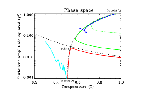
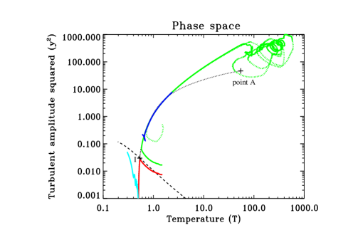
We select four initial conditions in each of the four quadrants that produce $(\bar{T},\bar{y})$ simulation trajectories qualitatively similar to the $(T,y)$ trajectories of the reduced model (thick coloured lines in Fig. 2).

3.1 Parameters

In order to make the comparison more quantitative, we need to specify the parameters $A$, $n$ and $W$. We use the estimated positions of the points ‘I’ and ‘A’ in the phase space $(\bar{T},\bar{y})$ in order to constrain the set of parameters that yields the best agreement. Indeed, the coordinates $(T_{\rm I},y_{\rm I})$ for the critical point ‘I’ completely specify the parameters $A$ and $W$ for a given value of $n$:

$$A=\sigma(T_{I})y_{I}^{1-n}$$ (16)

and

$$W=\frac{\Lambda(T_{\rm I})}{y_{\rm I}^{2}}\mbox{.}$$ (17)

The point ‘I’ is located at the crossing point between the separatrices, which are the asymptotes of the trajectories at early and late times. We estimate the position of the point ‘I’ for the simulations from the point at which the red and green trajectories diverge (see Fig. 2(a)).

In fact, the equations above also hold with $A$ indices : the active saturation point can also be used to fit the parameters. We find that $A=0.1$, $n=2$ and $W=1.2$ are values which satisfy both the conditions for points ‘I’ and ‘A’.

3.2 Phase diagram comparison

We plot the simulation trajectories in Fig.s 2(a) and 2(b). These should be compared with the trajectories in the first Fig. 1. As is plain, the qualitative agreement between the two methods is excellent. Particularly remarkable is the quantitative agreement near the critical point. This demonstrates that the relative values of thermal and turbulent time scales are accurately reproduced by the reduced model (the phase space trajectories are governed by the ratio between d$y/$d$t$ and d$T/$d$t$)). Fig. 2(b) also shows that the reduced model can describe the behaviour of the 3D system in a consistent way over a great range of magnitudes for $y$. The small value for the parameter $A$ actually helps the linear approximation to hold until larger amplitudes for $y$. The fastest linear modes are then likely to grow to large amplitudes relative to the other modes, which makes this system suitable to parasitic analyses such as in Goodman & Xu (1994) or Latter et al. (2009).

Our reduced model is in effect a 2 variable projection of a system with many more degrees of freedom. But surprisingly few details show the limits of the reduced model: only some trajectories exhibit self-crossing behaviour, for example when the sytem wanders near the saturation point ‘A’.

Figure 1: Phase diagram of the reduced model equations (9) and (10) with parameters $A=0.1$, $n=2$ and $W=1.2$. The separatrices of point ‘I’ are shown as dotted and dashed lines.

(a) Close up on the point ‘I’.

(b) Global view of the phase diagram.

Figure 2: Comparison with simulations of cubic domains. The separatrices of Fig. 1 are overlayed with five test trajectories $(\bar{T},\bar{y})$ in our simulations. The dotted green trajectory is the case ‘Ct’ simulation.

3.3 The route towards saturation

Here we focus on a typical cubic domain simulation, namely, the case ‘Ct’ simulation (see appendix A.5 for the nomenclature: case ‘Ci’ is isothermal, case ‘Cc’ has cooling, case ‘Ct’ has cooling and a temperature-dependent resistivity). But these comments are also valid for other cubic domain cases ‘Ci’ and ‘Cc’. From the initial conditions, the fastest growing mode is a vertical 2-channel flow which soon dominates. The mode grows in amplitude on a time scale no shorter than the orbital time scale. Meanwhile, the Alfvén speed increases and its crossing time through the box gets shorter and shorter. The total pressure balance across the simulation box is hence better and better realised. Therefore the growth of the 2-channel proceeds with a nearly uniform total pressure. The location of the two counter flowing channels corresponds to the nulls of magnetic pressure. Consequently, the thermal pressure must be maximal within the channels, and that pressure must increase as the amplitude of the mode rises. The result is a sharp increase in density at the location of the channels which get thinner and thinner due to mass conservation.

On either side of these channels, the magnetic field is almost uniform with same direction and opposite sign. The channels are also the current sheets where these two ordered fields reconnect. Ohmic heating is thus maximal at the location of these channels, which experience the highest temperature in the computational domain for non isothermal simulations (case ‘c’ or ‘t’).

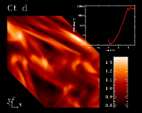
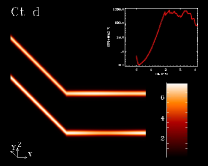
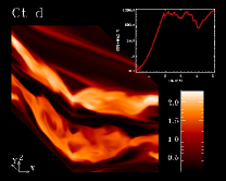
Fig. 3(b) illustrates the simulation ‘Ct’ during this phase of channel growth. The surprising sharpness of the channel feature is due both to the cube geometry of the box and to the linear filtering efficiency of case ‘t’. Indeed, when the resistivity increases (for lower temperatures) towards the marginal stability, fewer and fewer modes are available until only one mode is unstable. Strong channel features are therefore likely to be a characteristic of flows with a temperature close to the critical ‘I’ point. Also, the cubic geometry of the box does not allow for unstable parasitic modes as computed by Goodman & Xu (1994) to fit in the computational domain, so that the growing channel mode remains unhindered until very high amplitudes. As detailed in Latter et al. (2009) (for isothermal gases), it is then the shrinking of the channel width which decreases the wavelength of unstable parasites so that they finally fit in the box and start attacking the channel flow.

The growing process of the channel flow can also be viewed as the progressive spatial (as opposed to temporal as in the phase portrait) separation of the system into two phases: a high temperature region of dense and fast moving fluid with a disordered magnetic field (within the channels), and a lower temperature region of dilute quiet fluid with a strong ordered magnetic field (in between the channels). This is of course reminiscent of the phase separation described by our reduced model into an active and a quiet region. However, the two states are now coupled. For example, the fluid in the final quieter region does transport some angular momentum, as in the work of Fleming & Stone (2003) where a dead zone is activated by its neighbouring active zone. It also has a temperature significantly higher than the quiet state temperature $T_{0}$ due both to thermal diffusion and to the dissipation of the magnetic field. The partitioning of the medium into a dense and dilute phase, while the total pressure is kept uniform, resembles the classical Field thermal instability: high and low density regions appear at uniform thermal pressure. We recall that Balbus & Lesaffre (2008) interpreted the stability around the point ‘I’ thanks to a criterion similar to the Field criterion. The present study provides further evidence for this view.

(a) Initial conditions (after first transient evolution)

(b) The growing channel

(c) The steady state

(d) At a trough

Figure 3: Several density slices at various times of the simulation in case ‘Ct’. The evolution of the total kinetic plus magnetic energy ($\bar{y}^{2}$) in the perturbation is also given in the top right hand corner of each figure.

3.4 The saturated state

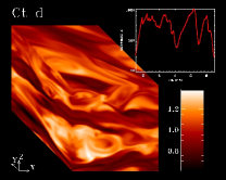
Even after the onset of the parasitic modes, both channels remain relatively well defined: we find that cubic domains lead to permanent channel flows (as witnessed in Latter et al. 2009). The parasites soon saturate, and the two channels remain flowing with travelling wave-like structures (as in saturated kink modes) or occasional plasmoids (saturated pinch modes) as illustrated on Fig. 3(c). These structures are reminiscent of the saturated kink and pinch modes that feed on magnetised jets as observed in Biskamp et al. (1998). The parasites’ perturbation of one channel are sometimes strong enough to diffuse and meet the parasites of the other channel, at which point some stronger coupling occurs, the channel flow slows and becomes more disordered, although two blocks with opposite velocities can still readily be identified as seen on Fig. 3(d). These events correspond to sudden dips in the evolution of the total energy contained in the computational domain. After a short while, two well defined channels reform, with their saturated parasites.

Simulations with shorter cooling time scales have less pressure support within the channel flows. They show thinner channels which break down sooner and yield lower saturation levels.

4 Other geometries

We have thus far limited the discussion to cubic domains, as these seem particularly fit for our reduced model. We briefly report here some of the potentially interesting behaviour we encountered in other geometries.

4.1 Bar results

Many MRI simulations have been performed in computational domains elongated in the azimuthal direction (Hawley et al. 1995; Fleming et al. 2000; Sano & Inutsuka 2001; Fromang & Papaloizou 2007; Fromang et al. 2007; Lesur & Longaretti 2007). Here we focus on the results we obtained in a similar geometry (our case ‘B’ with $L_{x}=1$ and $L_{y}=4$).

The bar geometry still does not allow for any Goodman & Xu (1994) parasites to fit in the computational domain for the channel flow of maximum growth. Indeed, the parasites’ wave vectors are restricted to a sector of angle less than $\pi/2$ encompassing the direction of the channel (Goodman & Xu 1994; Latter et al. 2009). The direction of the dominant channel flow is close to $\pi/4$ with respect to the direction axes. Hence the $x$-direction wavelength of a parasite needs to be bigger than the vertical extent of the channel in order to grow. As the channel gets thinner, however, compressible parasites may fit in the computational domain and attack the structure (Latter et al. 2009).

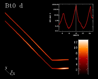
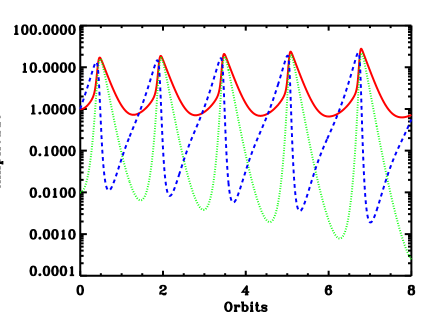
The chief difference between the cube and the bar is that in the latter there is enough room in the $y$-direction for the parasites to divert one channel into the path of the other, an event that leads to a dramatic collapse of the whole channel structure. Non-linear interactions quickly render the flow isotropic while reconnection brings the perturbation back to linear amplitudes. Depending on the overall resistivity (hence on the overall temperature), a new channel mode can or cannot grow. Depending on its thermal inertia, the system either enters a new cycle of eruption or decays. We can get immediate decay (case ‘Bt’), a few mild eruptions before decay (case ‘Bt’ with less initial seed for parasites), infinite sequence of mild eruptions (case ‘Bt’ with a longer cooling timescale), infinite sequence of moderate eruptions (case ‘Bi’ and ‘Bc’) or infinite sequence of strong eruptions (case ‘Bt0’, see Fig. 4). In case ‘Bt0’, the resistivity function is designed such that even for the radiative balance temperature there is still one unstable vertical MRI mode. In the next section, we devise a new reduced model which accounts for and sheds light on this wide variety of behaviour.

Figure 4: Density slices for case ‘Bt0’ on its way near the tip of a peak in total energy.

4.2 Eruptive reduced model

The previous discussion emphasises the role of the parasitic modes for the main growing mode which usually is a 2-channel mode. These parasites were described in Goodman & Xu (1994) and Latter et al. (2009) as a horizontal perturbation on top of a vertical main mode of evolution. Here we separate each field variable $X$ into its horizontally averaged contribution $\langle\,X\,\rangle_{z}$ (which only depends on the altitude $z$) and its remainder $\delta X=X-\langle\,X\,\rangle_{z}$. The component $\langle\,X\,\rangle_{z}$ naturally traces the main vertical ‘channel’ when one is dominating. And the component $\delta X$ can be thought of the ‘perturbations’ on top of this average profile.

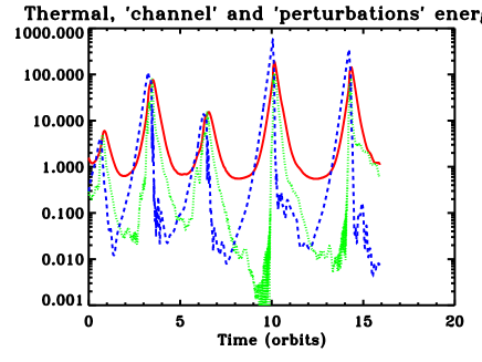
We now look at the separate evolution of the energies contained in each of the components. In particular, we monitor the magnetic energy in the ‘channel’ component

$$\bar{y}_{\rm c}^{2}=\frac{1}{4\pi}\langle\,\langle\,\mbox{\boldmath{$b$}}\,\rangle_{z}\mbox{\boldmath{$\cdot$}}\langle\,\mbox{\boldmath{$b$}}\,\rangle_{z}\,\rangle$$ (18)

and in the ‘perturbations’ component

$$\bar{y}_{\rm p}^{2}=\frac{1}{4\pi}\langle\,b^{2}-\langle\,\mbox{\boldmath{$b$}}\,\rangle_{z}\mbox{\boldmath{$\cdot$}}\langle\,\mbox{\boldmath{$b$}}\,\rangle_{z}\,\rangle$$ (19)

which are displayed on Fig. 5 along with the quantity $\bar{T}=\langle\,e\,\rangle$. We set the beginning of an eruptive cycle at a minimum of the ‘channel’ energy, where a dominant channel mode is just starting to emerge and grow. At this point ‘perturbations’ are still decaying roughly at an orbital rate and they dominate the total energy: the medium is vertically homogeneous in a statistical sense. The perturbations start to grow only after the channel amplitude has reached a certain threshold around 1 in our units. Then on the growth rate of the perturbations keeps increasing, in agreement with the idea that the growth of parasites is proportional to the channel amplitude (Goodman & Xu 1994; Latter et al. 2009). When the perturbations reach an amplitude comparable to the channel, the channel collapses and the medium is perturbation dominated. At this point, the system is in a state of decaying turbulence superimposed with spiral density waves, until the amplitudes become linear again, and a new channel mode emerges.

The description above naturally leads to a simple set of reduced equations where our former variable $y$ is now detailed into two components $y_{\rm c}$ and $y_{\rm p}$:

$$\frac{{\rm d}y_{\rm c}}{{\rm d}t}=\sigma(T)y_{\rm c}-Ay_{\rm c}^{2}y_{\rm p}\mbox{,}$$ (20)

$$\frac{{\rm d}y_{\rm p}}{{\rm d}t}=(y_{\rm c}-1)y_{\rm p}$$ (21)

and

$$\frac{{\rm d}T}{{\rm d}t}=Wy_{\rm c}^{2}-\frac{{\rm d}y_{\rm c}^{2}}{{\rm d}t}-\Lambda(T)\mbox{.}$$ (22)

The former non-linear saturation term is now replaced by a coupling term between the channel and the perturbations. The square exponent for $y_{\rm c}$ in $Ay_{\rm c}^{2}y_{\rm p}$ accounts for the observation that the breakup of a channel arises when two parasites interact. This simple reduced model is able to reproduce qualitatively each of the behaviours experienced in the simulations of the previous section, provided it is started with the right set of initial conditions for the channel and perturbation component (see Fig. 6 for case ‘Bt0’).

The main missing piece in this reduced model is how the decaying part of the cycle determines the starting amplitudes for the next cycle. The dice are rolled again during each phase of decaying turbulence.

Figure 5: Evolution of variables $\bar{T}$ (red, solid), $\bar{y}_{\rm c}^{2}$ (blue, dashed) and $\bar{y}_{\rm p}^{2}$ (green, dotted) (see text for definitions) in the case ‘Bt0’ simulation.

Figure 6: Evolution of variables $T$, $y_{\rm c}^{2}$ and $y_{\rm p}^{2}$ for the reduced equations (20)-(22) with $A=0.3$, $W=3/2$. The initial values are $T=1$, $y_{\rm c}=1$ and $y_{\rm p}=0.1$.

4.3 Slab results

Figure 7: Density slices for the case ‘Sc’ simulation at a point where a channel-like structure stands out.

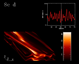
We also tested geometries with a slab aspect ratio $L_{x}=L_{y}=4$ while $L_{z}=1$. In this case, Goodman & Xu (1994) parasites can fit in the computational domain, but the amplitude of the resulting channels remain small so that a parasite analysis cannot be applied (see Latter et al. 2009). Case ‘St’ decays from the beginning, as for case ‘Bt’, but case ‘St0’ (with $\eta_{1}=0.007$) is similar to case ‘Sc’: intermittently, at the peak of the magnetic activity, a kinky channel-like structure (see Fig. 7) stands out. It washes out very quickly. This agrees with what Bodo et al. (2008) observe in their aspect ratio study.

The flow cannot be described as accurately with a simple model, as many modes of order 1 amplitude are present, all interacting with one another. However, the reduced model of equations (9) and (10) may still be used for qualitative comparison, but with a higher value for the constant $A$.

5 Summary and prospects.

We have performed Cartesian shearing-box simulations in conditions near marginal stability, which exist at the border between dead and active zones in accretion disks. The linear relative filtering at low amplitudes helps select prominent channel flows. This makes the system suitable for a description with simple reduced models which are able to account for general properties of the simulations such as internal energy, mechanical energy and momentum transport.

We investigated the influence of the thermal properties of the gas on the outcome of our simulations. The aspect ratio of our computational domain also has a very strong impact on their outcome. This is very likely due to the non-linear dynamics of interactions between various MRI modes (see Latter et al. 2009, for details).

Stratified and global simulations of disks are now required to determine which geometrical configuration is selected in real disks. Also, the presence of a mean vertical magnetic field in our simulations sets a preferred scale for the channel: simulations without zero net mean field still need to be investigated.

Last, we implied a dependence of the resistivity on the temperature which originally is mainly due to the electron fraction. The time scales for the recombination of electrons can be large and time-dependent chemistry has then to be accounted for. This eventually has to be included in order to link with the work of Ilgner & Nelson (2008), for example.

Appendix A Numerical Setup

A.1 Numerical method

Our code is basically the ZEUS3D code (Stone & Norman 1992a, b) with the shearing-box implemented as in Hawley et al. (1995), and we started from the version used by S. Fromang (Fromang & Papaloizou 2007) but amended it to better suit the problem at hand. We slightly improved the parallelisation scheme to increase its efficiency and accuracy.

We reset the mean magnetic field and the mean momentum to their initial values every 150 time steps, as in Silvers (2008). This prevents truncation errors for the mean momentum and magnetic fields from wandering too far from zero.

We split the momentum transport step for the Euler equation. We first transport the perturbed velocity $u$. This increases the accuracy of the Van-Leer slopes. Then we combine the advection of the mean shear with the Coriolis and tidal forces in an exact analytic rotation as in Section 3.3 of Gressel & Ziegler (2007). This increases the accuracy of the treatment of epicylic motions.

We do not use the artificial viscosity of ZEUS3D. We rather implement a physical viscous term which takes the same form as in equation (2). We rely on this term to degrade kinetic energy into heat and ensure total energy conservation (see below in Section A.5). We rewrite the resistive term in order to be able to use a non uniform resistivity $\eta$. The resistive criterion for the time-step control is made non-uniform accordingly. Similarly, note that viscosity is not assumed uniform in the present implementation of the viscous term, although we use it as a constant in the present study.

The diffusion step is done at the end of the standard ZEUS3D step and assumes the density is kept fixed. The cooling term follows and also assumes the density does not change. The dissipative source heat terms $\epsilon_{\rm d}$ (viscous and Ohmic) are computed along with the resistive and viscous terms and added as a constant to the cooling function $\Lambda_{\rm t}=\Lambda+\epsilon_{\rm d}$. We adopt a linear cooling function $\Lambda(T)=aT+b$ which allows us to compute the isochore evolution of the internal energy analytically. Time-step controls for the thermal diffusion and cooling are based on the diffusion time across a pixel $\Delta x^{2}/\chi$ (where $\Delta x$ is the size of a pixel) and the local cooling time-scale $\frac{{\rm d}\Lambda}{{\rm d}e}^{-1}$. These controls are never reached in practise (the limiting time is generally the Courant-Levy-Friedrich condition in the hottest pixel).

The version of the code used in this paper is available for download on the MAGNET website http://magnet.ens.fr.

A.2 Units

We use the orbital timescale $1/\Omega$ as our unit time. We use the vertical extent $L_{z}$ of the computational domain as our unit length. We use the mass initially contained in a cube of size $L_{z}$ as our unit mass, so that the initial average density in the box is $\langle\,\rho\,\rangle=1$ (the brackets denote volume averages over the full box). In addition, most of our runs begin with $\langle\,p\,\rangle=1$ in our units. The initial pressure scale height is therefore $H=1/\sqrt{\gamma}\simeq 0.77L_{z}$: the unit length is of the order of the initial pressure scale height. The scale height later varies as the average temperature in the box changes.

A.3 Thermal properties

In the isothermal case, the pressure is simply related to the density by $p=c_{0}^{2}\rho$ where $c_{0}$ is the initial sound speed in the non-isothermal runs. For the non-isothermal cases, the cooling function $\Lambda$ is a function of the temperature which we take to be linear

$$\Lambda(T)=aT+b.$$

In effect, this can be understood as the first order Taylor expansion of a more realistic cooling function around an intermediate temperature between the active and quiet states mentioned in the introduction.

The steady-state temperature $T_{0}$ results from the balance between viscous heating and radiative cooling. It may thus be written as

$$T_{0}=(\nu\frac{q^{2}\Omega^{2}}{4}-b)/a=T_{r}+\nu\frac{q^{2}\Omega^{2}}{4a}$$ (23)

which is slightly higher than the radiative equilibrium temperature $T_{r}=-b/a$ due to viscous heating. We fix the radiative equilibrium temperature to $T_{r}=1/2$ and hence adopt

$$\Lambda(T)=a(T-\frac{1}{2}).$$ (24)

The cooling time scale then depends only on the parameter $a$, which we set to $a=1$ in most of our runs. Larger values for $a$ yield similar results as in the isothermal case. Smaller values mean a longer cooling time $1/a$ and consequently a statistically stationary thermal state is reached after a longer integration time. Small values for $a$ also yield higher equilibrium temperatures which constrain the time-step to much lower values due to the Courant-Friedrich-Levy (CFL) condition.

A.4 Initial conditions

The mean vertical magnetic field is set to the value $B_{0}=\sqrt{2/400\pi}$ which corresponds to a plasma $\beta$ value of around $10^{2}$ when the average pressure is $\langle\,p\,\rangle=1$. For that value of the magnetic field, the wavelength of the MRI mode of maximum growth rate just fits in the vertical extent of the box (see Fig. 8).

Because the system supports two stationary states accessed by different initial conditions, we must then be careful how we characterise these. The initial configuration consists of a perturbation added to the stationary flow described above.

Random perturbations with low initial amplitude such as used by Hawley et al. (1995) lead to a long initial transient phase during which MRI modes grow and other components of the perturbation field decay, until the fastest growing MRI modes stand out. During this linear filtering phase, the temperature as well as the magnitude of the perturbation may change significantly.

In order to shorten this phase, we prepare the system in a state that is already linearly filtered to some extent. We choose to build the initial perturbation with a combination of some of the fastest growing modes and add a random seed. That mixture of a random perturbation and a selection of growing modes considerably shortens the initial transient phase. With this setup, we are indeed able to eliminate the initial strong first channel flow which appears in the time evolution of MRI shearing-box simulations.

We set the initial perturbation in the Fourier space of a larger domain and with a small scale cut off at intermediate scales. We then select only those modes which fit in the box. That way the same perturbation is used for runs with different geometries, different resolutions or different ways of sharing the domain between the processors units. To work in the Fourier space also allows to properly clean the divergence of the initial magnetic field.

Finally, we normalise the initial perturbation such that the maximum radial velocity is sonic (in fact, equal to 1 in our units). That high initial amplitude maximises our chances to first pick up the active state.

Figure 8: MRI dispersion relation for the vertical wave numbers in the conditions of the main simulations of this paper. Viscosity and resistivity are included. We display the real part of the fastest growing eigenvalue in units of the orbital time scale. The actual dispersion relation can be found in Lesaffre & Balbus (2007) , equation (16). The dotted line is for no ideal MHD. The solid line is for case ‘c’ ($\eta=\nu=2\times 10^{-3}$). The dashed line is for case ‘t’ with $T=0.5$ (radiative equilibrium) and the dash-dotted line is for $T=2/3$ (as in the initial conditions, which have $\langle\,p\,\rangle=1$). The vertical line indicates the vertical wavenumber of the box. The wavenumbers resolved by our simulations are right of this line, up to $k=64\pi$ for our standard resolution.

A.5 Parameter study

The main parameter we varied was the aspect ratio of the computational domain. The vertical size of the box $L_{z}$ was kept fixed to $L_{z}=1$. We set its radial size $L_{x}$ and azimuthal size $L_{y}$ to $L_{x}=L_{y}=1$ for the cube (first letter ‘C’), to $L_{x}=1$ and $L_{y}=4$ for a more classical azimuthal bar (first letter ‘B’) aspect ratio, and to $L_{x}=L_{y}=4$ for a slab (first letter ‘S’) aspect ratio.

We also changed the microphysical properties of the gas. We tested isothermal runs (second letter ‘i’), runs with constant resistivity and cooling (second letter ‘c’) and runs with a varying resistivity and cooling (second letter ‘t’). Some runs were performed with a lower resistivity and have a trailing zero in their coding name (simulation ‘Bt0’, for example, is a bar simulation with a varying resistivity lower than that of simulation ‘Bt’).

A.6 Resolution

We use an isotropic resolution as advised by Lesaffre & Balbus (2007). Our pixels are cubes of side length $\Delta x=1/64$ for our standard resolution. We halved that value for the case ‘t’ of each of the geometries for a resolution test on shorter integration times. The size of our simulations was then, in terms of zone numbers: $64^{3}$ for the cubes, $64\times 256\times 64$ for the bars and $256\times 256\times 64$ for the slabs (and eight times these numbers for the higher resolution tests). Our value for the Courant number (Lesaffre & Balbus 2007) ranges from 0.2 for cases ‘B’ and ‘S’ to 0.5 for case ‘C’. A low Courant number is necessary especially for case ‘t’ where large resistivity values can be obtained because our scheme uses an explicit resistive term. We aimed at fulfilling an integration time of a hundred of orbits. However, that time span could not be reached in case ‘C’. Case ‘Bt0’ is run for up to 330 orbits. In general, our simulations are run for time-step numbers of the order of a million up to six millions.

A.7 Dissipation and diffusion coefficients

Total energy is best conserved when the physical dissipation is much higher than the numerical dissipation. We use equation (50) of Lesaffre & Balbus (2007) with $\Delta x=1/64$, $\beta=100$, $C=0.5$ and $k=64\pi$ to get an upper bound estimate of the total numerical dissipation coefficient $\eta_{\rm N}+\nu_{\rm N}<5\times 10^{-3}$. Accordingly, we choose our minimal physical dissipation coefficients as $\eta_{0}=\nu=2\times 10^{-3}$. Our standard runs are hence only marginally resolved in places where strong gradients occur or where the magnetic field becomes very large. Our control runs with twice the resolution show that this does not impact our results except in case ‘C’, where we show only the results at a resolution of $128^{3}$. According to the same line of thought, we include thermal diffusion with $\chi=2\times 10^{-3}$ in cases ‘c’ and ‘t’ in order to avoid spurious thermal diffusion effects.

The resistivity in cases ‘i’ and ‘c’ is simply set to $\eta=\eta_{0}$. In case ‘t’, we adopted a resistivity of the form

$$\eta(T)=\eta_{0}+\eta_{1}T^{-3/2}$$ (25)

to mimic the power law dependence of the resistivity in a fully ionised plasma. The purpose was to test the validity of our simple dynamical system: both an active and a quiet state should be within reach of the system. Hence, the coefficient $\eta_{1}$ is chosen reasonably small (to avoid putting too much constraint on the time step due to high values of resistivity), while forcing all the MRI modes that fit in the computational to decay when the temperature is $T=0.5$. We use the values $\eta_{1}=1.2\times 10^{-2}$ for standard runs and $\eta_{1}=7\times 10^{-3}$ for lower resistivity runs (case ‘Bt0’, for example). The MRI dispersion relations for various realisations of the dissipation coefficients are plotted in Fig. 8.

References

- Balbus & Hawley (1991) Balbus S. A., Hawley J. F., 1991, ApJ, 376, 214
- Balbus & Lesaffre (2008) Balbus S. A., Lesaffre P., 2008, New Astronomy Review, 51, 814
- Biskamp et al. (1998) Biskamp D., Schwarz E., Zeiler A., 1998, Physics of Plasmas, 5, 2485
- Bodo et al. (2008) Bodo G., Mignone A., Cattaneo F., Rossi P., Ferrari A., 2008, Astron. Astrophys., 487, 1
- Fleming & Stone (2003) Fleming T., Stone J. M., 2003, ApJ, 585, 908
- Fleming et al. (2000) Fleming T. P., Stone J. M., Hawley J. F., 2000, ApJ, 530, 464
- Fromang & Papaloizou (2007) Fromang S., Papaloizou J., 2007, Astron. Astrophys., 476, 1113
- Fromang et al. (2007) Fromang S., Papaloizou J., Lesur G., Heinemann T., 2007, Astron. Astrophys., 476, 1123
- Fromang et al. (2002) Fromang S., Terquem C., Balbus S. A., 2002, M.N.R.A.S., 329, 18
- Gammie & Menou (1998) Gammie C. F., Menou K., 1998, ApJL , 492, L75+
- Goodman & Xu (1994) Goodman J., Xu G., 1994, ApJ, 432, 213
- Gressel & Ziegler (2007) Gressel O., Ziegler U., 2007, Computer Physics Communications, 176, 652
- Hawley et al. (1995) Hawley J. F., Gammie C. F., Balbus S. A., 1995, ApJ, 440, 742
- Ilgner & Nelson (2008) Ilgner M., Nelson R. P., 2008, Astron. Astrophys., 483, 815
- Latter et al. (2009) Latter H. N., Lesaffre P., Balbus S. A., 2009, M.N.R.A.S., 394, 715
- Lesaffre & Balbus (2007) Lesaffre P., Balbus S. A., 2007, M.N.R.A.S., 381, 319
- Lesur & Longaretti (2007) Lesur G., Longaretti P.-Y., 2007, M.N.R.A.S., 378, 1471
- Sano & Inutsuka (2001) Sano T., Inutsuka S.-i., 2001, ApJL , 561, L179
- Shakura & Syunyaev (1973) Shakura N. I., Syunyaev R. A., 1973, Astron. Astrophys., 24, 337
- Silvers (2008) Silvers L. J., 2008, M.N.R.A.S., 385, 1036
- Stone & Norman (1992a) Stone J. M., Norman M. L., 1992a, ApJS, 80, 753
- Stone & Norman (1992b) —, 1992b, ApJS, 80, 791