Effect of coupling between junctions on superconducting current and charge correlations in intrinsic Josephson junctions

Abstract

Charge formations on superconducting layers and creation of the longitudinal plasma wave in the stack of intrinsic Josephson junctions change crucially the superconducting current through the stack. Investigation of the correlations of superconducting currents in neighboring Josephson junctions and the charge correlations in neighboring superconducting layers allows us to predict the additional features in the current–voltage characteristics. The charge autocorrelation functions clearly demonstrate the difference between harmonic and chaotic behavior in the breakpoint region. Use of the correlation functions gives us a powerful method for the analysis of the current–voltage characteristics of coupled Josephson junctions.

The intrinsic Josephson junctions (IJJ) have a wide interest today due to the observed powerful coherent radiation from the stack of IJJ.ozyuzer The radiation is related to the region in the current–voltage characteristics (CVC) closed to the breakpoint region (BPR).sust1 ; prl ; prb The resistively and capacitively shunted junction (RCSJ) model and its different modifications are well known to describe the properties of single Josephson junctions, giving a clear picture of the role of quasiparticle and superconducting currents in the formation of CVC.kleiner ; likharev ; barone In the case of a stack of IJJ the situation is cardinally different. The system of the coupled Josephson junctions has a multiple branch structure and it has additional characteristics: the breakpoint current, the transition current to another branch and the BPR width. The breakpoint features were predicted theoretically and observed experimentally recently.irie We demonstrated that the CVC of the stack exhibits a fine structure in the BPR.prb2 The breakpoint manifests itself in the numerical simulations of the other authors as well.machida99

The breakpoint current characterizes the resonance point, at which the longitudinal plasma wave (LPW) is created in stacks, with a given number and distribution of the rotating and oscillating IJJ. These notions should be taken into account to have a correct interpretation of the experimental results. The investigation of the coupled system of Josephson junctions with a small value of the coupling parameter (as in the case of capacitive coupling), allowed us to understand in a significant way, the influence of the coupling between junctions on physical properties of the system. The capacitive coupling is realized in nanojunctions if the length of the junction is comparable to, or smaller than the Josephson penetration depth at zero external magnetic field. Coupling between intrinsic Josephson junctions leads to the interesting features which are absent in single Josephson junction. Still, the superconducting current in the coupled system of Josephson junctions with LPW has not been investigated in detail; this includes the role of the correlations of the superconducting currents in different junctions and the charge correlations on superconducting layers.

Here we study the phase dynamics of an IJJ stack in high-$T_{c}$ superconductor. The CVC of IJJ are numerically calculated in the framework of capacitively coupled Josephson junctions model with diffusion current.machida00 ; physC2 We find that the behavior of the superconducting current in the coupled system of Josephson junctions is essentially different from that of a single Josephson junction. It is demonstrated that superconducting current in the stack of IJJ reflects the main features of the breakpoint region; in particular, the fine structure in the CVC. We study various correlation functions in the characteristics, and observe that the correlations amongst the charge on different superconducting layers and correlations in the superconducting currents of different junctions lead to the detailed features of CVC in the BPR, and also provides additional information about the phase dynamics in the IJJ.

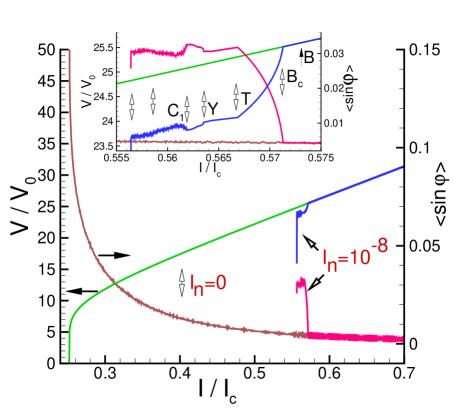
Figure 1: (Color online) The CVC and time averaged superconducting current $<\sin\phi_{l}>$ with no noise in current ($I_{n}=0$), and with noise amplitude $I_{n}=10^{-8}$. The inset shows an enlarged view of the BPR.

To find the CVC of the stack with N IJJ, we solve a system of N dynamical equations for the gauge–invariant phase differences $\varphi_{l}(t)\equiv\varphi_{l,l+1}(t)=\theta_{l+1}(t)-\theta_{l}(t)-\frac{2e}{\hbar c}\int^{l+1}_{l}dzA_{z}(z,t)$ between superconducting layers ($S$-layers), where $\theta_{l}$ is the phase of the order parameter in the S-layer $l$, and $A_{z}$ is the vector potential in the barrier. In our simulations we use a dimensionless time $\tau=t\omega_{p}$, where $\omega_{p}$ is the plasma frequency $\omega_{p}=\sqrt{2eI_{c}/\hbar C}$, ${I_{c}}$ is the critical current, and $C$ is the capacitance. The voltage is presented in units of $V_{0}=\hbar\omega_{p}/(2e)$, and the current in units of $I_{c}$. The system of equations has a form $\partial^{2}\varphi_{l}/\partial\tau^{2}=\sum_{l^{\prime}}\,A_{ll^{\prime}}[I-\sin\varphi_{l^{\prime}}-\beta\partial\varphi_{l^{\prime}}/\partial\tau]$ with matrix $A$ given in Ref. 4, for periodic and nonperiodic boundary conditions (BC). Using Maxwell’s equation $\emph{div}(\varepsilon E)=\rho/\varepsilon_{0}$, where $\varepsilon$ and $\varepsilon_{0}$ are relative dielectric and electric constants, we express the charge density $Q_{l}$ (we call it just charge) in the S-layer $l$ by the voltages $V_{l}$ and $V_{l+1}$ in the neighboring insulating layers $Q_{l}=Q_{0}\alpha(V_{l+1}-V_{l})$, where $Q_{0}=\varepsilon\varepsilon_{0}V_{0}/r_{D}^{2}$, and $r_{D}$ is the Debye screening length. Solution of the system of dynamical equations for the gauge–invariant phase differences between S-layers gives us the voltages $V_{l}$ in all junctions in the stack, and allows us to investigate the time dependence of the charge on each S-layer. The time dependence of the charge consists of time and bias current variations. We solve the system of dynamical equations for phase differences at fixed value of bias current I in some time $\tau$ domain $(0,T_{m})$ with a time step $\delta\tau$; we then change the bias current by the current step $\delta I$, and repeat the same procedure for the current $I+\delta I$ in the new time interval $(T_{m},2T_{m})$. The values of the phase and its time derivative at the end of the first time interval, are used as the initial conditions for the second time interval and so on. In our simulations we use $T_{m}=25000$, $\delta\tau=0.05$, $\delta I=10^{-5}$ and the dimensionless time $t_{r}$ is recorded as $t_{r}=\tau+T_{m}(I_{0}-I)/\delta I$, where $I_{0}$ is an initial value of the bias current. In this paper the CVC and the time dependence of charge oscillations in the S-layers are simulated at $\alpha=1$, $\beta=0.2$, using periodic BC. The details concerning the model and the numerical procedures have been presented before. physC2 ; prl ; prb

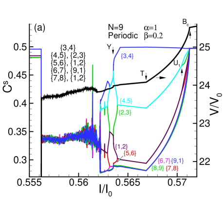
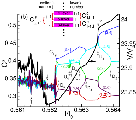
Figure 2: (Color online) (a) The correlation of superconducting currents in the stack with nine IJJ: the color curves plot the correlation functions $C^{s}_{j,j+1}=<\sin\varphi_{j}(\tau)\sin\varphi_{j+1}(\tau)>$ as a function of bias current for all $j$, the black curve shows the corresponding CVC. Label $\{2,3\}$, for instance, indicates the charge or current correlations between layers $2$ and $3$. (b) The enlarged region in the current interval (0.561, 0.564). Notations for current and charge correlation functions are also given in the inset.

Fig. 1 shows the CVC (green and blue curves) and the time averaged superconducting current $<\sin\phi_{l}>$ (brown and red curves ) without random noise in current, and with noise amplitude $10^{-8}$ for stack with nine IJJ. Our simulations of the CVC without noise gives us the value of the return current as $I_{r}/I_{c}=0.2517$, which coinciding with the value obtained from the RCSJ model. In fact, in this model the relation between the return and critical currents for $\beta<<1$ has the form $I_{r}/I_{c}=4\beta/\pi$, so that at $\beta=0.2$ we get $I_{r}/I_{c}=0.2546$. The superconducting current without noise demonstrates the standard increase before transition to the zero voltage state.likharev The noise in current helps create the LPW in the stack and influences the superconducting current; the particular value of noise is not very important. The creation of the LPW in the stack of junctions changes the CVC drastically, leading to the breakpoint and breakpoint region in CVC. Inset shows the enlarged part of the Fig. 1 in the breakpoint region, where arrows indicate the coincidence of the main features of CVC and the superconducting current. The point $B$ shows the point where a charge appears on the S-layers; point $B_{c}$ is a breakpoint on the CVC and it reflects the breakdown in the sharp increase of the charge’s value.prb2 If we take a sum of all equations $\ddot{\varphi_{l}}=(1-\alpha\triangledown^{2}_{l})(I-\beta\dot{\varphi_{l}}-\sin\varphi_{l})$ for N IJJ and then find its average in time, we obtain the equation $V=\frac{N}{\beta}(I-<sin\varphi>)$. This equation clearly shows why our results; namely, the $V$-curve and the $<sin\varphi>$-curve, demonstrate the same features.

To investigate the origin of the CVC features in the BPR, we study the correlations, $C^{s}_{j,j+1}$, of superconducting currents in the neighboring junctions $j$ and $j+1$: $C^{s}_{j,j+1}=<\sin\varphi_{j}(\tau)\sin\varphi_{j+1}(\tau)>=\lim_{(T_{m}-T_{i})\rightarrow\infty}\frac{1}{(T_{m}-T_{i})}\int_{T_{i}}^{T_{m}}{\sin\varphi_{j}(\tau)\sin\varphi_{j+1}(\tau)d\tau}$, where the brackets $<>$ mean averaging over time. The $C^{s}_{j,j+1}$ as functions of bias current $I/I_{c}$ are presented in Fig. 2a for $j=1,...,9$. All curves practically coincide in the interval starting from the breakpoint $B$ till point $B_{c}$. Then we observe regular, but different, behavior for different $j$ till point $C_{1}$, and then again $C^{s}_{j,j+1}$ is nearly the same for all $j$ in the chaotic region. As we can see in Fig. 2a, eight of these functions come in pairs as $(C^{s}_{4,5},C^{s}_{2,3})$, $(C^{s}_{5,6},C^{s}_{1,2})$, $(C^{s}_{6,7},C^{s}_{9,1})$, $(C^{s}_{7,8},C^{s}_{1,2})$; and one function, $C^{s}_{3,4}$ stands by itself. Let us note that because we consider a periodic BC, the number assigned to a junction is only a label. The black curve shows the outermost branch of the CVC of the stack with nine IJJ. We can see that the features of the correlation functions coincide with the features of CVC, i.e. they manifest themselves in the CVC curve. In Fig. 2b the part of Fig. 2a is plotted on an expanded scale. Arrows show the points where the features of $C^{s}_{j,j+1}$ coincide with those of CVC. In the inset to this figure we clarify the formation of the charge and superconducting current correlation functions by the diagram. Study of $C^{s}_{j,j+1}$ allows us to find new features in CVC which were not noticed in the previous studies.prb2 Particularly, in Fig. 2 we indicate the points $D_{2}$, $D_{3}$, $D_{4}$, and $D_{5}$ where the curves of the correlation functions diverge, and points $U_{1}$, $U_{2}$, $U_{3}$, $U_{4}$, where they converge.

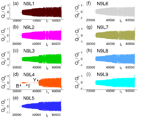
Figure 3: (Color online)Profile of time dependence of the charge in the S-layers in the stack with 9 IJJ at $\alpha=1$, $\beta=0.2$ and with periodic BC.

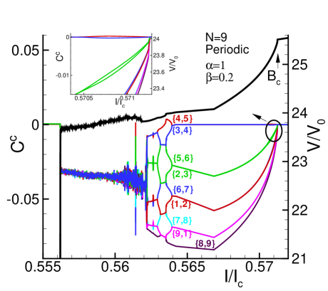
Figure 4: (Color online) The correlation of charge in the stack with nine IJJ: the color curves plot the correlation functions $C^{q}_{l,l+1}=<Q_{l}(\tau)Q_{l+1}(\tau))>$ for all $l$ as a function of bias current; the black curve shows the corresponding CVC. The inset shows the enlarged region near the point $B_{c}$.

To understand the origin of these features, we study the time dependence of charge in the superconducting layers. In Fig. 3 we show the profiles of the charge oscillations in all layers for the stack of nine IJJ. The odd number of junctions in the stack at periodic BC leads to the case where the charge dynamics in one layer, qualitatively differs from the others; namely, the layer 4 demonstrates a specific time dependence of the charge oscillations. We will refer to this layer as the “specific layer” or the sp-layer for short. The value of the charge on the sp-layer is smaller than on the other layers up to point $Y$, and practically staying at zero, in the interval from point $T$ till point $Y$. Such difference leads to the maximal value of $C^{s}_{3,4}$. The correlation function $C^{s}_{3,4}$ is different from the other correlation functions, because both phase differences in it ($\varphi_{34}$ and $\varphi_{45}$) are related to this unique layer. Any other correlation function has a partner which includes the same type of junction, for example $(C^{s}_{4,5}$ and $C^{s}_{2,3})$. Fig. 2b shows the enlarged region of Fig. 2a in the current interval (0.561,0.564). It clearly demonstrates that the features of the correlation functions reflect the features of CVC .

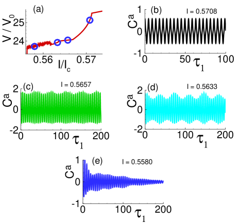
Figure 5: (Color online)(a) The CVC of the stack with nine IJJ; (b, c, d, e) The time dependence of the autocorrelation function $C^{a}_{5}$ in the different parts of the BPR at $I=0.57080,0.56570,0.56330$, and $0.55800$, respectively.

Let us investigate the charge correlations in the neighboring layers, using $C^{c}_{l,l+1}=<Q_{l}(\tau)Q_{l+1}(\tau))>=\lim_{(T_{m}-T_{i})\rightarrow\infty}\frac{1}{(T_{m}-T_{i})}\int_{T_{i}}^{T_{m}}{Q_{l}(\tau)Q_{l+1}(\tau)d\tau}$. Here we should emphasize that the index $l$ is a layer number. Fig. 4 presents the dependence of $C^{c}_{l,l+1}(I/I_{c})$ for different $l$ for the stack with nine IJJ at $\alpha=1$, $\beta=0.2$, with periodic BC. The negative sign of the $C^{c}_{l,l+1}$ is due to the $\pi$-mode of charge oscillations, so that the product of positive and negative charges gives us a negative sign for this function. Again, the correlation functions $C^{c}_{l,l+1}$ come in pairs: there are four pairs $(C^{c}_{4,5},C^{c}_{3,4}),(C^{c}_{5,6},C^{c}_{2,3}),(C^{c}_{6,7},C^{c}_{1,2}),(C^{c}_{7,8},C^{c}_{9,1})$; here, the correlation function that stands by itself is $C^{c}_{8,9}$ for layers 8 and 9, which are the farthest from the sp-layer (layer 4). The correlation functions $(C^{c}_{4,5}$ and $C^{c}_{3,4})$ between $T$ and $Y$ are close to zero, because the charge on the the sp-layer is close to zero in this interval. The inset shows the enlarged region around point $B_{c}$, where the charge on the sp-layer demonstrates its specific dynamics (see Fig. 3). The remarkable fact is that all pairs of current correlation functions $C^{s}_{j,j+1}$ and charge correlation functions $C^{c}_{l,l+1}$ form a loop reflecting this specific dynamics around this point! It means that the correlation functions reflect the correlations of phase dynamics amongst all layers and all junctions in the stack, even if the layers or junctions are far from each other. This is a demonstration of LPW in the system in other language. An interesting feature is observed in the chaotic region: At transition to the chaotic behavior (point $C_{1}$), the values of all correlation functions approach each other. The chaotic region will be discussed in detail elsewhere.

To distinguish the harmonic oscillations in the BPR from the chaotic behavior, we study the autocorrelation of the charge on the S-layers by the autocorrelation function $C^{a}_{l}=<Q_{l}(\tau)Q_{l}(\tau-\tau_{1})>=\lim_{(T_{m}-T_{i})\rightarrow\infty}\frac{1}{(T_{m}-T_{i})}\int_{T_{i}}^{T_{m}}{Q_{l}(\tau)Q_{l}(\tau-\tau_{1})d\tau}$. The autocorrelation function allows finding the repeating patterns (periodic signals) which have been buried under noise, or identifying the missing fundamental frequency in a signal, implied by its harmonic content. In Fig. 5a we show the CVC highlighted at $I=0.57080,0.56570,0.56330,$ and $0.55800$, where the time dependence of the autocorrelation function $C^{a}_{5}=<Q_{5}(\tau)Q_{5}(\tau-\tau_{1})>$ is investigated. Results are presented in Figs. 5(b)- 5(e). The different character of the autocorrelation function reflects the phase dynamics features in these parts of the BPR. At $I=0.5580$, inside the chaotic domain, we can clearly distinguish the periodic motion from the chaotic one, in that $C^{a}_{5}$ decays to zero with increasing time $\tau_{1}$.

In summary, the phase dynamics of intrinsic Josephson junctions in the high-$T_{c}$ superconductors is theoretically studied. We establish a correspondence between the features of current–voltage characteristics, and the superconducting current in the breakpoint region. We investigated the superconducting current in the coupled system of Josephson junctions with LPW and clarified the role of the superconducting current correlations in different junctions, in the formation of the total CVC. We demonstrated that the correlations of the superconducting currents in neighboring junctions and the correlations of the charge on superconducting layers manifest themselves as the features on the CVC, as a consequence of the phase dynamics in the breakpoint region. We showed that the correlation analysis is a powerful tool for the investigation of the CVC of the intrinsic Josephson junctions.

We thank R. Kleiner, K. Kadowaki, M. Suzuki, I. Kakeya, H. Wang, T. Hatano and F. Mahfouzi for helpful discussions. This research was supported by the Russian Foundation for Basic Research, grant 08-02-00520-a. M. Hamdipour acknowledges financial support from $BLTP$ and $IASBS$.

References

- (1) L.Ozyuzer et al, Science 318, 1291 (2007).
- (2) Yu. M. Shukrinov, F. Mahfouzi, N. F. Pedersen, Phys. Rev. B 75, 104508 (2007).
- (3) Yu. M. Shukrinov, F. Mahfouzi, Phys.Rev.Lett. 98, 157001 (2007).
- (4) Yu. M. Shukrinov, F. Mahfouzi, Supercond. Sci.Technol., 19, S38-S42 (2007).
- (5) W. Buckel, R. Kleiner, Superconductivity. Fundamentals and Applications, Wiley-VCH Verlag GmbH Co, KGaA, (2004).
- (6) A. Barone and J. Patterno, Physics and Applications of the Josephson effect, John Wiley and Sons (1982).
- (7) K. K. Likharev, Dynamics of Josephson Junctions and Circuits Gordon and Breach, New York (1986).
- (8) A. Irie, Yu. M. Shukrinov, G. Oya, Appl.Phys.Lett. 93, 152510, (2008).
- (9) Yu. M. Shukrinov, F. Mahfouzi, M. Suzuki, Phys. Rev. B 78, 134521 (2008).
- (10) M. Machida, T. Koyama, and M. Tachiki, Phys. Rev. Lett. 83, 4618 (1999).
- (11) M. Machida, T. Koyama, A. Tanaka and M. Tachiki, Physica C330, 85 (2000)
- (12) Yu. M. Shukrinov, F. Mahfouzi, P. Seidel. Physica C449, 62 (2006).