AGN with strong forbidden high-ionisation lines selected from the Sloan Digital Sky Survey

Abstract

We have defined a sample of 63 AGN with strong forbidden high-ionisation line (FHIL) emission. These lines, with ionisation potentials $\hbox{\raise 2.15277pt\hbox{$>\lower 4.56386pt\hbox{$\kern-10.70009pt{\sim}$}$}}100$ eV, respond to a portion of the spectrum that is often difficult to observe directly, thereby providing constraints on the extreme UV–soft X-ray continuum. The sources are selected from the Sloan Digital Sky Survey (SDSS) on the basis of their $[\mathrm{Fe}\,\mbox{{x}}]$$\lambda$6374Å emission, yielding one of the largest and the most homogeneous sample of FHIL-emitting galaxies. We fit a sequence of models to both FHILs ($[\mathrm{Fe}\,\mbox{{xi}}]$, $[\mathrm{Fe}\,\mbox{{x}}]$ and $[\mathrm{Fe}\,\mbox{{vii}}]$) and lower-ionisation emission lines ($[\mathrm{O}\,\mbox{{iii}}]$, $[\mathrm{O}\,\mbox{{i}}]$, $\mathrm{H}\alpha$, $[\mathrm{N}\,\mbox{{ii}}]$, $[\mathrm{S}\,\mbox{{ii}}]$) in the SDSS spectra. These data are combined with X-ray measurements from Rosat, which are available for half of the sample. The correlations between these parameters are discussed for both the overall sample and subsets defined by spectroscopic classifications. The primary results are evidence that: (1) the $[\mathrm{Fe}\,\mbox{{x}}]$ and $[\mathrm{Fe}\,\mbox{{xi}}]$ lines are photoionised and their strength is proportional to the continuum flux around 250 eV; (2) the FHIL-emitting clouds form a stratified outflow in which the $[\mathrm{Fe}\,\mbox{{x}}]$ and $[\mathrm{Fe}\,\mbox{{xi}}]$ source regions extend sufficiently close to the BLR that they are partially obscured in Seyfert 2s whereas the $[\mathrm{Fe}\,\mbox{{vii}}]$ source region is more extended and is unaffected by obscuration; (3) narrow-lined Seyfert 1s (NLS1s) tend to have the strongest $[\mathrm{Fe}\,\mbox{{x}}]$ flux (relative to lower-ionisation lines); and (4) the most extreme $[\mathrm{Fe}\,\mbox{{x}}]$ ratios (such as $[\mathrm{Fe}\,\mbox{{x}}]$/$[\mathrm{O}\,\mbox{{iii}}]$ or $[\mathrm{Fe}\,\mbox{{x}}]$/$[\mathrm{Fe}\,\mbox{{vii}}]$) are found in the NLS1s with the narrowest broad lines and appear to be an optical-band indication of objects with strong X-ray soft excesses.

1 Introduction

The forbidden high-ionisation emission lines (FHILs) have been known to exist in the optical spectra of Seyfert galaxies for more than 40 years (see Oke & Sargent, 1968 for the earliest published discussion of the $[\mathrm{Fe}\,\mbox{{x}}]$ species in NGC4151). Historically the $[\mathrm{Fe}\,\mbox{{x}}]$ line and other highly ionised species have been referred to in the literature as “coronal lines” because these species were first identified in the spectra of the solar corona. However, in this paper we will refer to them in terms of a specific physical property, i.e. as FHILs. We include in our definition of FHILs any forbidden line having an ionisation potential (IP) $\hbox{\raise 2.15277pt\hbox{$>\lower 4.56386pt\hbox{$\kern-10.70009pt{\sim}$}$}}100$ eV.

These lines are of interest for a variety of reasons. They define the nature of a galaxy in which they are detected as an AGN. This is because stellar spectra do not have sufficient high energy photons ($>100\ \mathrm{eV}$) to produce such species at detectable levels. Although SNRs can exhibit FHILs, these are distinguishable from those in AGN based on other properties, such as their profiles and velocity shifts with respect to other emission lines of lower ionisation. In AGN the FHILs tend to be broader and sometimes blueshifted compared to the profiles of the other emission lines (Appenzeller & Öestreicher, 1988; Erkens, Appenzeller & Wagner, 1997). Despite being well studied some fundamental questions are still not settled, such as whether the FHIL-emitting regions are powered by photoionisation or collisional processes. Also, the location of the zone in which the bulk of their line flux is emitted is not well established, although in some cases it has been possible to spatially resolve the region (see Rodríguez-Ardila et al., 2006 for a recent study). Their velocity widths imply a possible origin in a region contiguous with the innermost zones of the classic narrow line region (NLR), as defined by $[\mathrm{O}\,\mbox{{iii}}]$$\lambda$5007. This region can be spatially resolved be to about 10 parsecs for some nearby AGN (e.g., Kraemer, Schmitt & Crenshaw, 2008), and extends out to 100’s of parsecs and even kiloparsecs in some cases (e.g., Bennert et al., 2006a, b). By comparison the broad line region (BLR) is spatially unresolved, but is inferred from emission line reverberation mapping to be less than about a light month for a Seyfert of typical luminosity (Peterson et al., 2004).

On size scales between the BLR and the innermost resolved NLR lies the putative dusty molecular torus. This is believed to be a parsec-scale structure, with an inner edge that depends on the dust sublimation radius and may lie just beyond the BLR (Barvainis, 1987; Suganuma et al., 2006). Based on these generic components it has been suggested that the innermost FHIL-emitting regions lie somewhere between just beyond the BLR and the dusty torus. In addition to these qualitative considerations, the physical conditions of the FHILs, such as the density and temperature of the emitting gas derived from modeling their line flux ratios, has led to claims of an association with the so-called X-ray warm absorber (Porquet et al., 1999). This is an X-ray component very commonly identified in the low energy X-ray spectra of Seyfert 1s (Blustin et al., 2005). A consequence of these and other properties is that FHILs may be employed as diagnostics of outflows from the inner regions of the AGN, and may be a useful ingredient of wind models (Rodríguez-Ardila et al., 2006; Mullaney et al., 2009).

Unfortunately a current limitation in the study of FHILs and their potential use as diagnostics of the inner line emitting regions of AGN is that the samples available are quite small and heterogeneous, being limited to bright, relatively nearby AGN (De Robertis & Osterbrock, 1984; Veilleux, 1988; Erkens et al., 1997; Murayama & Taniguchi, 1998, hereafter MT98; Nagao, Taniguchi & Murayama, 2000, hereafter NTM00). In this paper we introduce a new sample of significant size, constructed using the FHILs themselves as a selection criterion, the first time this technique has been employed. This larger sample will enable meaningful statistical tests to be performed on the FHILs and other properties of the AGN, and also to consider the relevance of AGN classifications such as Seyfert 1, Seyfert 2, and narrow line Seyfert 1 (Sy1, Sy2, and NLS1, respectively).

The sample selection is presented in §2. In §3 we describe the models and the fitting procedure applied to the optical data, and how we interpret both these models and X-ray count rates from Rosat. The results of these analyses are characterized in §4. In §5 we consider the implications of these results. Our findings are summarized in §6.

We adopt cosmological parameters from WMAP ($H_{\circ}=71\ \mathrm{km\,s^{-1}}\,\mathrm{Mpc}^{-1}$, $\Omega_{\mathrm{M}}=0.27$ and $\Omega_{\Lambda}=0.73$; Spergel et al., 2003). The wavelengths reported throughout this paper are those observed in air, not the vacuum wavelengths reported in the Sloan Digital Sky Survey (SDSS; York et al., 2000) catalog. This is for consistency with the vast majority of previous literature on this subject. Reported errors for fitted parameters are $\pm 1\sigma$ confidence intervals; when average properties of samples are discussed, we generally provide both the $\pm 1\sigma$ confidence interval of the mean value and the RMS scatter about the mean.

2 Sample selection

Our objective is to construct a sample of galaxies selected based on their strong FHIL emission. We do not make the a priori assumption that such emission will only be found in AGN. Because FHIL emission is relatively rare, we require a large spectroscopic survey from which to draw our sample. For this the SDSS is ideally suited, in that the current release (DR6, Adelman-McCarthy et al., 2008) provides uniform quality spectra for nearly 900,000 galaxies and AGN spanning more than 2 steradians (6860 square degrees).

The SDSS data processing pipeline (Stoughton et al., 2002) fits simple Gaussian models to a set of features in each spectrum, yielding a database of line parametrizations that is readily searched. Unfortunately this database does not include any optical FHILs. However, it does include both lines of the $[\mathrm{O}\,\mbox{{i}}]\lambda\lambda 6300,6364$ doublet. $[\mathrm{O}\,\mbox{{i}}]\lambda 6364$ is close enough to $[\mathrm{Fe}\,\mbox{{x}}]\lambda 6374$ that the SDSS line model will represent a blend of these two features if this FHIL is present. In such cases the pipeline models of the $[\mathrm{O}\,\mbox{{i}}]$ lines will neither share the same profile nor have a 3:1 flux ratio, as expected from atomic physics. Thus $[\mathrm{Fe}\,\mbox{{x}}]$-emitting galaxies may be found by identifying SDSS spectra whose $[\mathrm{O}\,\mbox{{i}}]\lambda 6364$ models show evidence of contamination.

We construct a sample of candidate $[\mathrm{Fe}\,\mbox{{x}}]$-emitting galaxies by applying the following selection criteria to the SDSS database:

1. identified as either a galaxy or a quasar by the SDSS spectroscopic pipeline (SPECCLASS = 2 or 3, respectively);

2. redshift $<0.40$ to ensure that $\mathrm{H}\alpha$ lies within the observed 3800–9200 Å wavelength range;

3. $\mathrm{H}\alpha$ Gaussian model width $\sigma<50$ Å to minimize the contamination of $[\mathrm{O}\,\mbox{{i}}]$ by any broad H$\alpha$ wings;

4. $[\mathrm{O}\,\mbox{{i}}]$ doublet models with significance greater than 10-$\sigma$ in each line to ensure well-defined profiles;

5. $[\mathrm{O}\,\mbox{{i}}]\lambda 6364$ line centroids shifted by $\geq 1.5$ Å relative to $[\mathrm{O}\,\mbox{{i}}]\lambda 6300$ (in the emitted frame; equivalent to $>1.0$ SDSS spectral bin), which is indicative of $[\mathrm{Fe}\,\mbox{{x}}]$ blends.

The resulting $\sim$200 candidates were then visually inspected to identify the highest-quality sources and to eliminate spectra with obvious contamination around 6370 Å (sky subtraction artefacts or any unmodeled $\mathrm{H}\alpha$ components that introduce steep gradients). Sources were selected for the final sample that have one or more pieces of unambiguous corroborating evidence of FHIL emission: (1) a distinct emission feature near 6374 Å, (2) $[\mathrm{O}\,\mbox{{i}}]+[\mathrm{Fe}\,\mbox{{x}}]$ blend significantly broader than $[\mathrm{O}\,\mbox{{i}}]\lambda 6300$, (3) $[\mathrm{O}\,\mbox{{i}}]$ doublet ratio inconsistent with 3, and/or (4) prominent $[\mathrm{Fe}\,\mbox{{vii}}]\lambda 6087$ emission.

Table 1: SDSS galaxies selected by $[\mathrm{Fe}\,\mbox{{x}}]$ emission (see §2 for column descriptions).

ID	RA $\pm$ Dec (J2000.0)	SC	Class	r	$z_{\mathrm{[\mathrm{S}\,\mbox{{ii}}]}}$	$v_{\mathrm{corr}}$	$\Delta\lambda_{[\mathrm{O}\,\mbox{{i}}]6364}$		$\Delta\mathrm{FWHM}$		$[\mathrm{O}\,\mbox{{i}}]$ ratio		Alternative IDs
1	00:18:52.47+01:07:58.5	2	S1.9	18.10	0.0640	-47	7.$\pm$	2.	12.$\pm$	4.	0.70$\pm$	0.09
2	01:10:09.01–10:08:43.4	3	NLS1	17.60	0.0583	-66	3.$\pm$	3.	15.$\pm$	4.	0.57$\pm$	0.07	1WGA J0110.1-1008
3	02:33:01.24+00:25:15.0	2	S2	15.39	0.0224	19	4.3$\pm$	0.4	2.9$\pm$	1.0	0.80$\pm$	0.08	1WGA J0232.9+0025
4	07:31:26.69+45:22:17.5	3	S1.5	17.84	0.0921	-4	3.$\pm$	4.	11.$\pm$	6.	1.06$\pm$	0.13
5	07:36:38.86+43:53:16.5	2	S2	17.96	0.1140	37	3.5$\pm$	1.3	8.$\pm$	3.	1.55$\pm$	0.17
6	07:36:50.08+39:19:55.2	2	S2	19.12	0.1163	-13	5.8$\pm$	1.8	13.$\pm$	4.	0.98$\pm$	0.10
7	08:07:07.18+36:14:00.5	2	S2	16.23	0.0324	-21	8.5$\pm$	1.0	19.0$\pm$	1.6	0.25$\pm$	0.03	IC 2227
8	08:11:53.16+41:48:20.0	2	S2	18.35	0.0999	-96	5.6$\pm$	0.7	1.6$\pm$	1.9	1.45$\pm$	0.14
9	08:29:30.59+08:12:38.1	3	S1.0	17.24	0.1295	-95	6.5$\pm$	1.0	15.$\pm$	3.	0.54$\pm$	0.05
10	08:30:45.37+34:05:32.1	3	S1.5	16.66	0.0624	-39	5.0$\pm$	0.9	13.$\pm$	2.	0.89$\pm$	0.09
11	08:30:45.41+45:02:35.9	3	S1.0	17.84	0.1825	-49	3.$\pm$	6.	16.$\pm$	5.	0.22$\pm$	0.02
12	08:36:58.91+44:26:02.4	3	S1.0	15.71	0.2544	15	2.0$\pm$	1.2	10.6$\pm$	1.3	0.60$\pm$	0.05	Q 0833+446; RBS 711
13	08:42:15.30+40:25:33.3	2	S2	16.85	0.0553	2	8.$\pm$	2.	15.$\pm$	3.	1.05$\pm$	0.12
14	08:46:22.54+03:13:22.2	3	S1.0	17.48	0.1070	-22	8.8$\pm$	0.5	7.9$\pm$	1.2	0.67$\pm$	0.06
15	08:53:32.22+21:05:33.7	2	S2	17.73	0.0719	-32	6.2$\pm$	1.1	7.$\pm$	2.	1.07$\pm$	0.11
16	08:57:40.86+35:03:21.7	3	S1.5	19.25	0.2752	46	3.4$\pm$	1.6	10.8$\pm$	1.6	0.77$\pm$	0.08
17	08:58:10.64+31:21:36.3	2	S2	18.23	0.1389	-15	6.1$\pm$	1.5	13.4$\pm$	1.7	1.03$\pm$	0.10
18	09:17:15.00+28:08:28.2	3	S1.5	18.08	0.1045	-37	10.0$\pm$	1.2	19.$\pm$	9.	0.35$\pm$	0.04
19	09:18:25.79+00:50:58.4	3	S1.5	18.16	0.0871	-43	6.6$\pm$	0.7	11.$\pm$	2.	0.79$\pm$	0.09
20	09:23:43.00+22:54:32.6	3	NLS1	15.65	0.0330	51	8.2$\pm$	0.6	16.8$\pm$	0.9	0.37$\pm$	0.03	MCG +04-22-42
21	09:42:04.79+23:41:06.9	3	S1.5	15.92	0.0215	-49	7.0$\pm$	0.7	4.5$\pm$	1.8	1.19$\pm$	0.14	PGC 027720
22	10:01:49.52+28:47:09.0	2	S1.9	17.32	0.1849	17	6.3$\pm$	0.9	7.$\pm$	2.	1.22$\pm$	0.08	3C 234
23	10:17:18.26+29:14:34.1	3	S1.5	16.71	0.0492	-66	3.8$\pm$	0.7	13.$\pm$	2.	0.38$\pm$	0.05
24	10:22:35.15+02:29:30.5	2	NLS1	18.71	0.0701	-84	8.$\pm$	5.	8.$\pm$	9.	0.76$\pm$	0.09
25	10:34:38.60+39:38:28.3	2	NLS1	16.80	0.0435	-107	3.3$\pm$	0.4	6.6$\pm$	1.2	0.37$\pm$	0.02	KUG 1031+398
26	10:55:19.54+40:27:17.5	3	S1.5	17.49	0.1201	-27	2.3$\pm$	1.0	16.$\pm$	2.	0.90$\pm$	0.09	Mrk 1269
27	11:02:43.20+38:51:52.6	2	NLS1	18.89	0.1186	-19	8.3$\pm$	1.3	18.8$\pm$	1.7	0.84$\pm$	0.09	1WGA J1102.7+3851
28	11:07:04.52+32:06:30.0	3	S1.5	17.64	0.2425	104	2.$\pm$	3.	2.9$\pm$	1.3	1.25$\pm$	0.06
29	11:07:16.49+13:18:29.5	3	S1.5	18.35	0.1848	-44	3.5$\pm$	0.7	10.$\pm$	2.	0.56$\pm$	0.07
30	11:07:56.55+47:44:34.8	3	S1.0	16.98	0.0727	3	5.$\pm$	5.	16.$\pm$	2.	0.40$\pm$	0.05
31	11:09:29.10+28:41:29.2	2	S2	17.20	0.0329	-77	5.$\pm$	3.	18.$\pm$	11.	0.55$\pm$	0.05
32	11:26:02.46+34:34:48.2	2	S1.9	17.92	0.1114	-78	1.9$\pm$	0.7	4.1$\pm$	1.9	1.18$\pm$	0.14
33	11:31:07.10+11:58:59.3	3	S1.0	17.58	0.0910	2	4.3$\pm$	0.9	10.$\pm$	3.	0.78$\pm$	0.09
34	11:39:17.17+28:39:46.9	2	S2	17.05	0.0234	-11	9.5$\pm$	1.5	1.$\pm$	4.	0.81$\pm$	0.09
35	11:42:16.88+14:03:59.7	2	S2	16.44	0.0208	-48	6.4$\pm$	0.2	6.9$\pm$	0.5	0.95$\pm$	0.04
36	11:52:26.30+15:17:27.6	3	S1.5	17.91	0.1126	2	2.$\pm$	2.	12.$\pm$	3.	1.15$\pm$	0.12
37	11:57:04.84+52:49:03.7	2	S2	16.78	0.0356	-39	6.3$\pm$	0.8	12.1$\pm$	1.7	1.32$\pm$	0.10
38	12:04:22.15–01:22:03.3	3	S1.0	17.58	0.0834	2	6.$\pm$	4.	17.$\pm$	9.	0.53$\pm$	0.07
39	12:07:35.06–00:15:50.3	2	S2	18.84	0.1104	-28	2.6$\pm$	1.9	7.$\pm$	4.	1.46$\pm$	0.17
40	12:09:32.94+32:24:29.3	3	NLS1	17.94	0.1303	97	3.5$\pm$	0.8	11.$\pm$	2.	1.32$\pm$	0.13
41	12:10:44.28+38:20:10.3	3	S1.0	15.63	0.0230	-43	10.0$\pm$	1.4	15.$\pm$	2.	0.82$\pm$	0.08	KUG 1208+386
42	12:29:03.50+29:46:46.1	2	S1.5	18.45	0.0821	-166	3.7$\pm$	1.3	6.$\pm$	3.	1.02$\pm$	0.12
43	12:29:30.41+38:46:20.7	2	S2	18.20	0.1024	-39	2.4$\pm$	0.6	0.5$\pm$	1.6	1.52$\pm$	0.16
44	12:31:49.08+39:05:30.2	3	S1.5	17.50	0.0683	-39	6.$\pm$	6.	5.$\pm$	7.	0.86$\pm$	0.10
45	12:41:34.25+44:26:39.2	2	gal	18.87	0.0419	18	10.$\pm$	5.	1.$\pm$	10.	0.33$\pm$	0.03
46	13:11:35.66+14:24:47.2	3	NLS1	17.03	0.1140	-61	1.7$\pm$	0.8	17.8$\pm$	0.7	0.32$\pm$	0.03
47	13:13:05.69–02:10:39.3	3	S1.0	16.70	0.0838	-20	3.$\pm$	3.	17.5$\pm$	1.6	0.38$\pm$	0.04
48	13:13:48.96+36:53:58.0	3	S1.5	17.59	0.0670	-66	6.4$\pm$	0.7	10.$\pm$	2.	0.78$\pm$	0.08
49	13:16:39.75+44:52:35.1	2	S2	17.37	0.0911	-55	2.9$\pm$	0.6	10.1$\pm$	1.9	1.03$\pm$	0.06	1WGA J1316.6+4452
50	13:19:57.07+52:35:33.8	2	NLS1	17.92	0.0922	-69	6.0$\pm$	0.8	15.4$\pm$	1.9	0.48$\pm$	0.03	RBS 1249
51	13:23:46.00+61:04:00.2	2	S2	17.58	0.0715	-36	2.5$\pm$	0.8	4.7$\pm$	1.0	2.37$\pm$	0.13
52	13:46:07.71+33:22:10.8	3	S1.0	17.45	0.0838	-44	5.$\pm$	5.	17.$\pm$	4.	0.60$\pm$	0.07
53	13:55:42.76+64:40:45.0	3	NLS1	16.73	0.0753	-42	3.$\pm$	2.	15.$\pm$	4.	0.48$\pm$	0.02	VII Zw 533
54	14:34:52.46+48:39:42.8	3	S1.0	15.93	0.0365	-8	6.$\pm$	3.	17.3$\pm$	1.5	0.60$\pm$	0.06	NGC 5683; Mrk 474
55	15:32:22.32+23:33:25.0	2	S2	17.46	0.0465	-50	8.$\pm$	2.	14.$\pm$	2.	1.37$\pm$	0.14
56	15:35:52.40+57:54:09.5	3	S1.0	15.21	0.0304	15	4.7$\pm$	1.0	17.1$\pm$	1.1	0.62$\pm$	0.06	Mrk 290
57	16:09:48.21+04:34:52.9	2	S2	17.77	0.0643	-91	6.7$\pm$	0.9	5.$\pm$	2.	1.15$\pm$	0.07
58	16:13:01.63+37:17:14.9	3	S1.0	16.46	0.0695	12	6.1$\pm$	1.6	16.0$\pm$	1.3	0.53$\pm$	0.05	KUG 1611+374B
59	16:18:44.85+25:39:07.7	3	NLS1	16.94	0.0479	9	8.$\pm$	3.	18.$\pm$	7.	0.36$\pm$	0.04
60	16:35:01.46+30:54:12.1	3	S1.5	17.33	0.0543	-1	9.1$\pm$	1.6	16.$\pm$	4.	0.43$\pm$	0.04
61	20:58:22.14–06:50:04.4	3	NLS1	18.22	0.0740	-58	4.8$\pm$	0.7	8.1$\pm$	1.7	0.86$\pm$	0.10
62	22:02:33.85–07:32:25.0	3	NLS1	17.05	0.0594	-6	4.0$\pm$	0.6	11.3$\pm$	1.6	0.76$\pm$	0.06
63	22:15:42.30–00:36:09.8	3	S1.0	17.30	0.0994	-30	3.7$\pm$	1.0	11.$\pm$	2.	0.98$\pm$	0.10
64	23:56:54.30–10:16:05.5	3	S1.5	16.59	0.0740	-77	2.2$\pm$	0.3	14.6$\pm$	0.9	0.42$\pm$	0.02

The final sample, consisting of 64 strong $[\mathrm{Fe}\,\mbox{{x}}]$-emitting galaxies, is presented in Table 1. The columns are: (1) ID number; (2) J2000.0 coordinates; (3) SDSS SPECCLASS value (“SC”; 2 = galaxy, 3 = quasar); (4) our spectral classification (see §3.2.5); (5) $r$ magnitude integrated over a 3-arcsec diameter region (SDSS fiber magnitude); (6) redshift defined from the observed wavelengths of the $[\mathrm{S}\,\mbox{{ii}}]$ doublet (see §3.2.2); (7) correction to recessional velocity due to difference between SDSS- and $[\mathrm{S}\,\mbox{{ii}}]$-defined $z$ ($\mathrm{km\,s^{-1}}$; $\Delta v_{\mathrm{corr}}<0$ if $z_{\mathrm{SDSS}}<z_{\mathrm{[\mathrm{S}\,\mbox{{ii}}]}}$); (8–10) SDSS $[\mathrm{O}\,\mbox{{i}}]$ model parameters that provide evidence of blended $[\mathrm{Fe}\,\mbox{{x}}]$: (8) offset of $[\mathrm{O}\,\mbox{{i}}]\lambda 6364$ model centroid from expected position ($\Delta\lambda_{[\mathrm{O}\,\mbox{{i}}]6364}=\lambda_{[\mathrm{O}\,\mbox{{i}}]6364}-\lambda_{[\mathrm{O}\,\mbox{{i}}]6300}-63.472$ Å, where wavelengths are measured in the emitted frame in Å); (9) difference in widths of $[\mathrm{O}\,\mbox{{i}}]$ doublet line models ($\Delta\mathrm{FWHM}=\mathrm{FWHM}_{6364}-\mathrm{FWHM}_{6300}$, in Å), and (10) flux ratio of $[\mathrm{O}\,\mbox{{i}}]\lambda 6300/[\mathrm{O}\,\mbox{{i}}]\lambda 6364$; and (11) alternative common names (including WGA catalogue IDs for the four sources detected in pointed Rosat observations but not in the Rosat All-Sky Survey). These represent a diverse range of Seyfert objects: 26 type 1s (including 12 NLS1s), 19 intermediate types (16 of type 1.5 and 3 of type 1.9), and 18 type 2 Seyferts (our working definitions for these spectral types are described in §3.2.5). In addition we found one galaxy with an unusual spectrum that is not Seyfert-like. It is listed in Table 1 (object 45, spectral type “gal”) but is not included in the rest of this paper; it is discussed in detail in a separate study (Ward et al. in preparation). We note that 27 out of these 64 objects are spectroscopically classified by the SDSS pipeline as galaxies and not quasars: the one non-Seyfert galaxy, all of the Sy2 and Sy1.9 sources, plus one Sy1.5 (source 42) and four NLS1s (sources 24, 25, 27, and 50).

This is one of the largest and by far the most homogeneous sample of AGN with strong FHILs to date. However, we note that this sample is by no means complete. There are certainly many other galaxies with strong $[\mathrm{Fe}\,\mbox{{x}}]$ emission in the SDSS catalogue that have been excluded by the $[\mathrm{O}\,\mbox{{i}}]$ significance or the $\mathrm{H}\alpha$ width criteria. Our selection criteria introduce biases against Seyfert 1s with the broadest permitted lines and any FHIL-emitting sources dominated by lines with lower IPs (e.g., with low $[\mathrm{Fe}\,\mbox{{x}}]/[\mathrm{Fe}\,\mbox{{vii}}]$ ratios). This is in addition to any biases inherited from the SDSS spectroscopic survey (e.g., the photometric criteria used by SDSS to select spectroscopic targets coupled with the fact that we directly observe the AGN continuum flux in Sy1s and not in Sy2s means that SDSS-selected type 1 objects will extend to higher redshifts and may include less intrinsically powerful nuclei). Nevertheless, the size and relative homogeneity of this sample makes it useful for testing correlations between FHIL features and other properties.

3 Analysis

In this paper we focus our attention on the strongest FHILs and the most prominent other lines available for low redshift objects within the SDSS spectral band. In the wavelength range $3500<\lambda<9000$ Å, the strongest observed lines with IPs $\hbox{\raise 2.15277pt\hbox{$>\lower 4.56386pt\hbox{$\kern-10.70009pt{\sim}$}$}}100$ eV are all species of iron: $[\mathrm{Fe}\,\mbox{{vii}}]\lambda 6087$, $[\mathrm{Fe}\,\mbox{{x}}]\lambda 6374$ and $[\mathrm{Fe}\,\mbox{{xi}}]\lambda 7892$. Other FHILs in this range include $[\mathrm{Fe}\,\mbox{{xiv}}]\lambda 5303$, $[\mathrm{Fe}\,\mbox{{xi}}]\lambda 3987$, and several $[\mathrm{Fe}\,\mbox{{vii}}]$ lines (notably ones at 5721, 5276, 5159, 4893, 3967 and 3586 Å; see, e.g., Osterbrock, 1981; Appenzeller & Öestreicher, 1988; Erkens et al., 1997), but we do not measure these because they are not as strong, some are blended with other features, and the shorter wavelength lines will be more strongly affected by any dust that is present. In addition to the three strongest iron FHILs, we also measure $\mathrm{H}\alpha$ and the following lower-ionization forbidden lines: $[\mathrm{O}\,\mbox{{iii}}]\lambda 5007$, $[\mathrm{O}\,\mbox{{i}}]\lambda\lambda 6300,6364$, $[\mathrm{N}\,\mbox{{ii}}]\lambda\lambda 6548,6583$, and $[\mathrm{S}\,\mbox{{ii}}]\lambda\lambda 6718,6730$.

3.1 Spectral fitting procedure

We designed a set of idl scripts to fit a series of models to the SDSS spectra. In order to minimize the complexity of these models, we made separate analyses of six bands around $[\mathrm{O}\,\mbox{{iii}}]$, $[\mathrm{Fe}\,\mbox{{vii}}]$, $[\mathrm{O}\,\mbox{{i}}]$+$[\mathrm{Fe}\,\mbox{{x}}]$, $\mathrm{H}\alpha$+$[\mathrm{N}\,\mbox{{ii}}]$, $[\mathrm{S}\,\mbox{{ii}}]$ and $[\mathrm{Fe}\,\mbox{{xi}}]$. In each interval we first fit a low-order polynomial to establish the local continuum. This may include both true continuum and other broad components, notably the wings of any broad $\mathrm{H}\alpha$ components that sometimes extend to wavelengths near $[\mathrm{Fe}\,\mbox{{x}}]$ and $[\mathrm{S}\,\mbox{{ii}}]$. We therefore used a third-order polynomial in these two bands to allow for some curvature in the continuum model and a second-order polynomial in the other bands. This local continuum is subtracted from the data before applying a sequence of emission line models.

The sequence of models applied to each emission line starts with a single Gaussian. The initial fitting is done with the line profile parameters (width and centroid) fixed at assumed values in order to minimize the number of free parameters. Next, the profiles are allowed to vary (within limits: doublets are assumed to have the same profiles; additional constraints are described below) and the best-fitting parameters are determined. We then try adding a second Gaussian, using $\chi^{2}$ statistics to test whether the added component provides a significantly better description of the data. In the case of $\mathrm{H}\alpha$ we also try adding a third Gaussian to the model, once again testing whether the added component is significant. The most detailed model that offers a significantly improved fit is adopted as the best-fitting model, provided that it passes a final visual inspection (described in the next section). The best-fitting models are presented online in Tables 7–16. In Fig. 1 we demonstrate the best-fitting line models for one of our sample members in the $[\mathrm{O}\,\mbox{{iii}}]$, $[\mathrm{Fe}\,\mbox{{vii}}]$, $[\mathrm{Fe}\,\mbox{{x}}]$(+$[\mathrm{O}\,\mbox{{i}}]$), and $\mathrm{H}\alpha$(+$[\mathrm{N}\,\mbox{{ii}}]$) bands (the $[\mathrm{S}\,\mbox{{ii}}]$ and $[\mathrm{Fe}\,\mbox{{xi}}]$ line models are not shown because these are fitted with only a single Gaussian and are not blended).

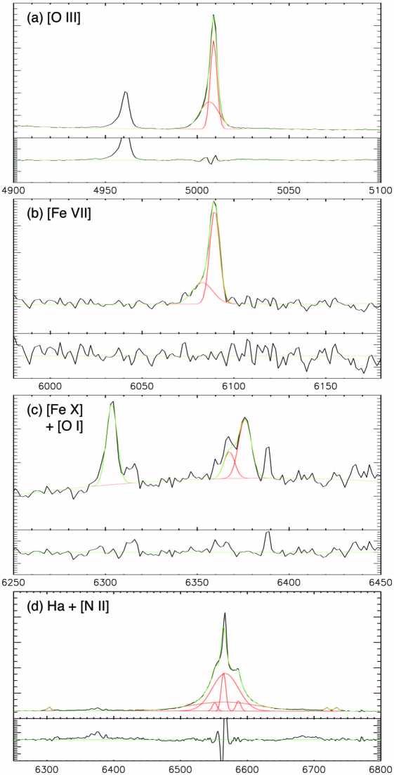
Figure 1: A demonstration of the multi-component line models as applied to the NLS1 VII Zw 533 (source 53). Pairs of panels show the data with the best-fitting models overlaid and the residuals after the models have been subtracted. From the top down are the $[\mathrm{O}\,\mbox{{iii}}]$, $[\mathrm{Fe}\,\mbox{{vii}}]$, $[\mathrm{Fe}\,\mbox{{x}}]$, and $\mathrm{H}\alpha$ bands. Red curves are the individual model components; green curves are either the total model (in the data plots) or the zero line (in the residual plots). Note the distinct blue wing in both the $[\mathrm{O}\,\mbox{{iii}}]$ and $[\mathrm{Fe}\,\mbox{{vii}}]$ line profiles. Wavelengths are in the emitted frame (as defined by SDSS redshifts) and the flux density scale is arbitrary.

Some notes on details of the line-fitting process:

• Two-component forbidden line models: The double-Gaussian model provides a significantly improved fit to the $[\mathrm{O}\,\mbox{{iii}}]$ line for every member of our sample. The same cannot be said of the $[\mathrm{Fe}\,\mbox{{vii}}]$ line, which is found to require a second component in only 14 cases. The other forbidden line data generally do not require a second component so only single Gaussian models are used. We note that the use of a mix of single- and double-Gaussian models to fit $[\mathrm{Fe}\,\mbox{{vii}}]$ does not introduce a strong systematic effect, as the fluxes of most compound models differ from those of best-fitting single Gaussians by no more than 15 per cent, which is comparable to the uncertainty in the measurements. The advantage of sometimes using the two-component model is a more accurate characterization of the profile of the core of the $[\mathrm{Fe}\,\mbox{{vii}}]$ lines.

• Blended lines: In order to separate blended lines, additional constraints were applied. In the case of the $[\mathrm{O}\,\mbox{{i}}]$+$[\mathrm{Fe}\,\mbox{{x}}]$, we first determined the best-fitting parameters for the $[\mathrm{O}\,\mbox{{i}}]$$\lambda$6300 line. We then assumed an $[\mathrm{O}\,\mbox{{i}}]$$\lambda$6364 model with the same width and velocity shift and 1/3 the intensity of $[\mathrm{O}\,\mbox{{i}}]$$\lambda$6300 and fitted the $[\mathrm{Fe}\,\mbox{{x}}]$ model to the remaining flux. A similar process was used to deblend $\mathrm{H}\alpha$ and the $[\mathrm{N}\,\mbox{{ii}}]$ doublet. If the $[\mathrm{N}\,\mbox{{ii}}]$ models are not constrained, they will sometimes include a significant amount of $\mathrm{H}\alpha$ flux. This is especially problematic when the width of $\mathrm{H}\alpha$ is $\sim 1500\ \mathrm{km\,s^{-1}}$ because the $[\mathrm{N}\,\mbox{{ii}}]$ models can effectively slice off the broad line wings, resulting in $\mathrm{H}\alpha$ models that are systematically too narrow. To mitigate this tendency, a Gaussian fitted to $[\mathrm{O}\,\mbox{{i}}]$$\lambda$6300 was used as a template for the narrow line emission profile. The $[\mathrm{N}\,\mbox{{ii}}]$ models were assigned the same width and velocity shift as $[\mathrm{O}\,\mbox{{i}}]$, with only the intensity allowed to vary. These intensities were re-fitted with each successive $\mathrm{H}\alpha$ model.

• $\mathrm{H}\alpha$ model components: Up to three Gaussian components are used to model the $\mathrm{H}\alpha$ lines; the third is discarded as unnecessary in 21 instances. One of the Gaussians is forced to have the same width and velocity shift as the narrow line template defined by $[\mathrm{O}\,\mbox{{i}}]$ (see previous comment on blended lines). Thus, the $\mathrm{H}\alpha$ model is guaranteed to have at least one component with the characteristics of the NLR.

• $[\mathrm{Fe}\,\mbox{{xi}}]$ measurements: SDSS does not provide spectral coverage at the wavelength of $[\mathrm{Fe}\,\mbox{{xi}}]$ for eight of our sample members (six are at $z>0.16$; two others have gaps in their data). Of the remaining 55 AGN spectra, 36 provide $[\mathrm{Fe}\,\mbox{{xi}}]$ detections with $>99$ per cent confidence despite the increased noise due to OH sky lines at these wavelengths.

3.2 Optical parameter analysis

3.2.1 Rejection of spurious models

A final check of the best-fitting models was made to identify any dubious line model components. The most common mode of failure was when a second (or third) component of $[\mathrm{Fe}\,\mbox{{vii}}]$ or $\mathrm{H}\alpha$ became extremely broad to account for residual continuum flux. In such cases we reverted to the best-fitting parameters of a previous, less complex model. Apart from these cases, there were four other best-fitting models that were revised after inspection. In two instances (sources 40 and 48) $[\mathrm{Fe}\,\mbox{{xi}}]$ models were discarded because they were found to be fitted to sky line residuals. For source 28, a Sy1.5 with a very broad $\mathrm{H}\alpha$ component, the $[\mathrm{Fe}\,\mbox{{x}}]$ Gaussian was used to model part of the continuum and had to be re-fitted manually. In one other object (source 5, a Seyfert 2 with relatively simple line profiles) one of the $\mathrm{H}\alpha$ components was fitted to $[\mathrm{N}\,\mbox{{ii}}]\lambda 6583$; to correct this, its flux has been reassigned to the $[\mathrm{N}\,\mbox{{ii}}]$ line.

3.2.2 Line velocity shifts and redshift redefinition

The velocity shifts ($v_{\mathrm{sh}}$) of the emission lines are measured relative to the recession velocities of their host galaxies. Hence, a negative velocity shift indicates a reduced recession velocity of a line-emitting region. We interpret $v_{\mathrm{sh}}<0\ \mathrm{km\,s^{-1}}$ as outflow velocities along our line of sight, although we cannot rule out the possibility of emission from infalling clouds approaching from the far side of the AGN.

In order to measure $v_{\mathrm{sh}}$ with the highest possible precision, care must be taken in how the systemic redshifts are defined. The SDSS pipeline uses multiple methods to measure redshifts; the final value is defined by the method that yields the highest confidence measurement. However, there can be systematic differences between the redshift values determined by these methods (e.g., when emission lines are dominated by outflows and are used as the basis of the redshift measurement). Such systematics may be present at the few hundred $\mathrm{km\,s^{-1}}$ level even when the SDSS pipeline reports that the measurements are mutually consistent (as is the case for 46 out of 63 sample members). Therefore, if we are to measure $v_{\mathrm{sh}}$ with precision better than a few hundred $\mathrm{km\,s^{-1}}$ and avoid systematic effects, we must ensure that a consistent definition of redshift is used for our entire sample.

Ideally we would define systemic redshifts from the stellar properties of the host galaxies, but not all of our sample members have measurable absorption features. Instead, we base our definition upon the centroid wavelengths of the $[\mathrm{S}\,\mbox{{ii}}]$ doublet. This doublet is chosen because it has a low IP and a low critical density ($N_{cr}$). Therefore, amongst the emission lines available in all our spectra, this is the feature most likely to be dominated by regions farthest from the central engine, where the influence of the AGN is expected to be weakest. Thus, the $[\mathrm{S}\,\mbox{{ii}}]$ lines should be more closely related than any other available feature to the kinematics of the ISM of the host galaxy. However, it is possible that these lines may sometimes arise in outflowing gas. In such cases the line centroid will not accurately indicate the systemic velocity of the host if the observed velocity structure is not symmetric (e.g., if there is a bi-conal outflow and we do not integrate comparable amounts of flux from both sides).

The change from SDSS-defined to $[\mathrm{S}\,\mbox{{ii}}]$-defined redshifts results in a range of $v_{\mathrm{sh}}$ adjustments from -166 to +$103\ \mathrm{km\,s^{-1}}$. The median adjustment is $-34\ \mathrm{km\,s^{-1}}$, so the redshift redefinition tends to increase the outflow velocities. All $v_{\mathrm{sh}}$ values reported in this paper are measured relative to the $[\mathrm{S}\,\mbox{{ii}}]$-defined redshifts. It is worth noting that the $v_{\mathrm{sh}}$ values of $[\mathrm{O}\,\mbox{{i}}]$ and the core of $[\mathrm{O}\,\mbox{{iii}}]$ (defined in the next section) agree very well with those of $[\mathrm{S}\,\mbox{{ii}}]$, with mean values of $0\pm 4$ and $-5\pm 5\ \mathrm{km\,s^{-1}}$, respectively. This agreement is somewhat surprising because the critical densities of these lines are larger by factors of $10^{3}$ and $10^{2.5}$, so their emission is expected to be dominated by different regions.

3.2.3 $[\mathrm{O}\,\mbox{{iii}}]$ and $[\mathrm{Fe}\,\mbox{{vii}}]$ components

For every source in this sample the two-component line model provided a significantly better fit to the $[\mathrm{O}\,\mbox{{iii}}]$ profile than did the single-Gaussian model. In most cases the second component was used to represent asymmetric line profiles. We therefore adopt the nomenclature of “core” and “wing” components of the line ($[\mathrm{O}\,\mbox{{iii}}]_{C}$ and $[\mathrm{O}\,\mbox{{iii}}]_{W}$, respectively), with the core defined to be the component whose centre is closer to the peak of the overall profile. The core is invariably the Gaussian with the smaller FWHM. With this definition, 53 $[\mathrm{O}\,\mbox{{iii}}]$ lines have blue wings, 6 have red wings, and 5 have components separated by less than 1/4 pixel ($<17\ \mathrm{km\,s^{-1}}$; see Table 12).

Unlike $[\mathrm{O}\,\mbox{{iii}}]$, double-Gaussian models seldom provide a significantly better fit to the $[\mathrm{Fe}\,\mbox{{vii}}]$ lines. When two Gaussians are used, we again divide them into core and wing components ($[\mathrm{Fe}\,\mbox{{vii}}]_{C}$ and $[\mathrm{Fe}\,\mbox{{vii}}]_{W}$). In all cases we find that $[\mathrm{Fe}\,\mbox{{vii}}]_{W}$ is both broader and bluer than $[\mathrm{Fe}\,\mbox{{vii}}]_{C}$. In the remaining 49 cases the single Gaussian model is used as $[\mathrm{Fe}\,\mbox{{vii}}]_{C}$ (hence $[\mathrm{Fe}\,\mbox{{vii}}]_{1G}=[\mathrm{Fe}\,\mbox{{vii}}]_{C}$ for most sample members). The best-fitting $[\mathrm{Fe}\,\mbox{{vii}}]$ models are presented in Table 10. This table includes the best-fitting single Gaussian models for all sample members, even those for which the double Gaussian model provides a significant improvement, in order to provide a model that is uniform across the entire sample. We use the notation $[\mathrm{Fe}\,\mbox{{vii}}]_{1G}$ when we refer to the single Gaussian models for the entire sample.

We note that there is a potential degeneracy when deblending the core and wing line components. If too much or too little flux is attributed to the core, then the width and velocity shift of the wing can be affected. At best this degeneracy introduces an additional uncertainty in the parameters of the individual components, contributing noise to the data; at worst it can introduce systematic effects that skew the average values across the sample. Thus, the core and wing components may be thought of as a possibly non-physical parametrization of an asymmetric line profile. As such, the properties of these individual components, especially those of the wing, may best be interpreted qualitatively. Although the exact details of these components may be suspect, they do provide a more accurate description of the shape of the line profile than a single Gaussian model could. Moreover, the flux of the combined model provides a better measure of the actual flux from the line. We therefore consider the sum of the component fluxes to be a robust measure of the line strength, and will emphasize this in the ensuing discussion. Hereafter, we use the subscript “_T” when referring to this combined flux.

3.2.4 $\mathrm{H}\alpha$ components

The $\mathrm{H}\alpha$ lines are fitted with up to three Gaussian components. These models generally have one narrow, one intermediate, and one broad component (a third component is rejected in only 21 instances). However, sometimes more than one of these had a FWHM comparable to that of $[\mathrm{O}\,\mbox{{i}}]$. Clearly, the intermediate-width component did not consistently represent a distinct region: sometimes it was unambiguously broad ($\mathrm{FWHM}>2000\ \mathrm{km\,s^{-1}}$), other times it was used to fine-tune the modeling of the NLR contribution to $\mathrm{H}\alpha$. We therefore decided to combine the Gaussians into two $\mathrm{H}\alpha$ components: $\mathrm{H}\alpha_{N}$, interpreted as the NLR contribution to $\mathrm{H}\alpha$, combines all components not much broader than $[\mathrm{O}\,\mbox{{i}}]$, and $\mathrm{H}\alpha_{B}$, the BLR contribution, includes all Gaussians substantially broader than $[\mathrm{O}\,\mbox{{i}}]$. The ratios of $\mathrm{H}\alpha$ component FWHM over $[\mathrm{O}\,\mbox{{i}}]$ FWHM almost always had values $\leq 1.3$ or $\geq 2.8$ (Fig. 2), so these thresholds were used to define $\mathrm{H}\alpha_{N}$ and $\mathrm{H}\alpha_{B}$ components. When $\mathrm{H}\alpha_{N}$ or $\mathrm{H}\alpha_{B}$ consist of more than one component, the flux used is the sum of the components and the profile is that of the highest-flux Gaussian. As with $[\mathrm{O}\,\mbox{{iii}}]_{T}$ and $[\mathrm{Fe}\,\mbox{{vii}}]_{T}$, we use $\mathrm{H}\alpha_{T}$ when referring to the combined flux of all the $\mathrm{H}\alpha$ components.

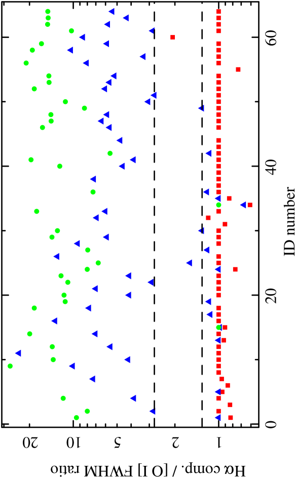
Figure 2: Ratios of the $\mathrm{H}\alpha$ component widths over $[\mathrm{O}\,\mbox{{i}}]$ FWHM. Red squares, blue triangles and green circles represent the FWHM ratios of progressively broader $\mathrm{H}\alpha$ Gaussian components over $[\mathrm{O}\,\mbox{{i}}]$$\lambda$6300. Dashed lines are drawn at ratios of 1.3 and 2.8. Components that fall below the lower line are assigned to $\mathrm{H}\alpha_{N}$ whilst those above the higher line are assigned to $\mathrm{H}\alpha_{B}$; the few points between are considered individually. By construction, all $\mathrm{H}\alpha$ models include one Gaussian with the FWHM of $[\mathrm{O}\,\mbox{{i}}]$ unless this component is found to not be significant.

3.2.5 Spectroscopic classifications

The first challenge in establishing the spectroscopic classifications of our sample members is to separate the Seyfert 2s from the other Seyfert types. Simply using the FWHM of the broadest $\mathrm{H}\alpha$ component is problematic because in several Sy2s (the ones with strong $[\mathrm{O}\,\mbox{{iii}}]$ wings), the $\mathrm{H}\alpha$ models include a weak but statistically significant broad component. This component appears to be real but its width (FWHM sometimes $2000\ \mathrm{km\,s^{-1}}$ or more; cf. Table 16) is non-physical, in that it is fitted to the blended, otherwise-unmodeled blue wings of $\mathrm{H}\alpha$+$[\mathrm{N}\,\mbox{{ii}}]$ emission from the NLR. Another complication is that the $\mathrm{H}\alpha_{B}$ FWHM of the narrowest NLS1s is comparable to the broadest $\mathrm{H}\alpha_{N}$ lines amongst the Sy2s. Instead of using $\mathrm{H}\alpha$ FWHM, we use two line flux ratios, $[\mathrm{N}\,\mbox{{ii}}]$/$\mathrm{H}\alpha_{T}$ and $[\mathrm{O}\,\mbox{{iii}}]_{T}$/$\mathrm{H}\alpha_{T}$. The total $\mathrm{H}\alpha$ flux is a strong discriminator between Sy2 and other Seyfert types because lines that include a broad component usually have much more flux, but neither ratio alone is sufficient as a single parameter to separate the Sy2s because there is some overlap with other Seyfert types. However, following the approach of Baldwin, Phillips & Terlevich (1981), we find that the Sy2s are very well separated from all other AGN in the plane defined by these two ratios (Fig. 3; see also Zhang et al., 2008). All of the Sy2s in the present study are bounded by $\log([\mathrm{O}\,\mbox{{iii}}]_{T}/\mathrm{H}\alpha_{T})>0$ and $\log([\mathrm{N}\,\mbox{{ii}}]/\mathrm{H}\alpha_{T})>-0.5$. These ratios have not been corrected for reddening, which would tend to increase the $[\mathrm{O}\,\mbox{{iii}}]_{T}$/$\mathrm{H}\alpha_{T}$ values. However, Sy2s generally require the largest corrections, so accounting for reddening would strengthen their separation in this plane.

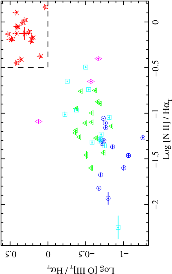
Figure 3: Line diagnostic ratios used to separate Sy2s from other Seyferts. Sy2s (red stars) are bounded by $\log([\mathrm{O}\,\mbox{{iii}}]_{T}/\mathrm{H}\alpha_{T})>0$ and $\log([\mathrm{N}\,\mbox{{ii}}]/\mathrm{H}\alpha_{T})>-0.5$. The other sample members are classified as Sy1.9s (magenta diamonds), Sy1.5s (green triangles), NLS1s (cyan squares), and Sy1.0s (blue circles) according to their H line profiles.

Once the Sy2s are separated, the remaining type 1 AGN are classified based on the properties of their Balmer lines. The 12 sources with $\mathrm{H}\alpha_{B}\ \mathrm{FWHM}<2200\ \mathrm{km\,s^{-1}}$ are defined to be NLS1; the other type 1 Seyferts collectively comprise the broad-lined Seyferts (BLS1). Note that the division between NLS1s and BLS1s is somewhat arbitrary but we apply it here to compare with previous work and to see if other properties distinguish this sub-class. The BLS1s are subdivided into three groups: the ones with very little $\mathrm{H}\alpha_{N}$ emission are Sy1.0s (based upon the fraction of the overall $\mathrm{H}\alpha$ flux in the $\mathrm{H}\alpha_{N}$ component, with a subjectively-chosen threshold of no more than 8 per cent); most of the rest, with larger $\mathrm{H}\alpha_{N}$/$\mathrm{H}\alpha_{B}$ ratios, are Sy1.5s; the few with no clear broad component at $\mathrm{H}\beta$ are classified as Sy1.9s. The final tally of spectral types is 14 Sy1.0s, 12 NLS1s, 16 Sy1.5s, 3 Sy1.9s, and 18 Sy2s.

3.2.6 Estimates of dust reddening

The measured line fluxes are not corrected for reddening. The impact of dust is generally small, as most sample members appear to have very little reddening (based upon both the Balmer decrements and the shapes of the continua). Furthermore, it is difficult to measure the Balmer decrement reliably for many type 1 Seyferts because of the difficulty in separating $\mathrm{H}\alpha_{N}$ from $\mathrm{H}\alpha_{B}$, rendering any correction uncertain. Amongst the few spectra that do appear to be affected by dust, the most reddened objects are sources 7, 13, and 32; two Sy2s and a Sy1.9 for which we estimate $A_{V}=3.3$, 3.5 and 2.9, respectively. In no other Seyfert have we found $A_{V}>2.2$. To mitigate the effect of any uncorrected reddening, we will place some emphasis on comparisons of lines that are close in wavelength. For instance, with $A_{V}<2.2$ for the rest of the sample, the effect upon $[\mathrm{Fe}\,\mbox{{vii}}]$/$[\mathrm{Fe}\,\mbox{{x}}]$ ratios will be $\leq 10$ per cent and is always smaller than the measurement uncertainty.

3.2.7 Summary of the final line profile models

The final set of models adopted for the discussion that follows is summarized in Table 2. The $[\mathrm{O}\,\mbox{{iii}}]$ and $[\mathrm{Fe}\,\mbox{{vii}}]$ lines fitted with two Gaussians are organized into core and wing components, as described in §3.2.3. The $\mathrm{H}\alpha$ lines are fitted with up to three Gaussians which are then combined into two components, “broad” and “narrow” ($\mathrm{H}\alpha_{B}$ and $\mathrm{H}\alpha_{N}$; §3.2.4). For these lines, which at least sometimes include more than one component, we use the subscript “_T” (i.e., $[\mathrm{O}\,\mbox{{iii}}]_{T}$, $[\mathrm{Fe}\,\mbox{{vii}}]_{T}$ and $\mathrm{H}\alpha_{T}$) to refer to the combined fluxes of all components. The remaining lines (the $[\mathrm{O}\,\mbox{{i}}]$, $[\mathrm{N}\,\mbox{{ii}}]$ and $[\mathrm{S}\,\mbox{{ii}}]$ doublets, $[\mathrm{Fe}\,\mbox{{x}}]$ and $[\mathrm{Fe}\,\mbox{{xi}}]$) are fitted with single-Gaussian models. For many of the NLR lines, the model parameters are linked to each other. In particular, the $[\mathrm{O}\,\mbox{{i}}]\lambda 6364$ model is completely defined by the fit to $[\mathrm{O}\,\mbox{{i}}]\lambda 6300$. Because of this, unless $6364$ Å is specified, any mention of $[\mathrm{O}\,\mbox{{i}}]$ will implicitly refer to the stronger line at $6300$ Å.

Table 2: Final spectral line models used for analysis.

Emission	IP	Log $N_{cr}$	Comp	Details of
line	(eV)	($\mathrm{cm}^{-3}$)	count	final fit
$[\mathrm{O}\,\mbox{{iii}}]\lambda 5007$	35.1	5.8	2	Core & wing components
$[\mathrm{Fe}\,\mbox{{vii}}]\lambda 6087$	99.1	7.6	1–2	Only 14 final models
				include wing component
$[\mathrm{O}\,\mbox{{i}}]\lambda 6300$	—	6.3	1	All parameters free
$[\mathrm{O}\,\mbox{{i}}]\lambda 6364$	—	6.3	1	Pars. defined by $[\mathrm{O}\,\mbox{{i}}]\lambda 6300$
$[\mathrm{Fe}\,\mbox{{x}}]\lambda 6374$	233.6	9.7	1	All parameters free
$[\mathrm{N}\,\mbox{{ii}}]\lambda 6548$	14.5	4.9	$\left.\rule{0.0pt}{11.40965pt}\right\}1\ \ \$	$[\mathrm{N}\,\mbox{{ii}}]$ $v_{\mathrm{sh}}$ & FWHM
$[\mathrm{N}\,\mbox{{ii}}]\lambda 6584$	14.5	4.9		defined by $[\mathrm{O}\,\mbox{{i}}]\lambda 6300$
$\mathrm{H}\alpha$	—	—	2	Broad & narrow comps.
$[\mathrm{S}\,\mbox{{ii}}]\lambda 6716$	10.4	3.2	$\left.\rule{0.0pt}{11.40965pt}\right\}1\ \ \$	$[\mathrm{S}\,\mbox{{ii}}]$ doublet fitted with
$[\mathrm{S}\,\mbox{{ii}}]\lambda 6731$	10.4	3.6		single $v_{\mathrm{sh}}$ & FWHM
$[\mathrm{Fe}\,\mbox{{xi}}]\lambda 7892$	262.1	10.4	1	36 $[\mathrm{Fe}\,\mbox{{xi}}]$ det., 19 non-det.

$[\mathrm{O}\,\mbox{{i}}]\lambda 6300$ is used as a template for the parameters of the $[\mathrm{O}\,\mbox{{i}}]\lambda 6364$ model in order to deblend $[\mathrm{O}\,\mbox{{i}}]$+$[\mathrm{Fe}\,\mbox{{x}}]$, and for the profile of the NLR when fitting $\mathrm{H}\alpha$+$[\mathrm{N}\,\mbox{{ii}}]$. Columns are (1) line ID; (2) ionisation potential (eV); (3) log of the critical density at $T=10^{4}$ K for the forbidden transition lines (cm^-3); (4) number of model components used; (5) details regarding parameter constraints and (in the cases of $[\mathrm{Fe}\,\mbox{{vii}}]$ and $[\mathrm{Fe}\,\mbox{{xi}}]$) the frequency with which models are considered significant.

3.3 Rosat X-ray data

Half of our sample members (32 out of 63) appear in catalogues of soft X-ray sources detected with the Rosat PSPC. We convert the PSPC count rates to fluxes using the PIMMS tool from HEASARC, assuming a power law model with a photon index $\Gamma=1.5$ and an intervening absorption column of $n_{H}=3\times 10^{20}\ \mathrm{cm}^{-2}$ at $z=0$. It is well established that NLS1s often have much steeper soft X-ray spectral indices than other Seyfert galaxies (Boller, 2000), so we also consider the effect of using $\Gamma=3.0$ for the NLS1s. Given these assumed models, the conversion from RASS count rates to fluxes in the full 0.1–2.4 keV Rosat band is equivalent to multiplicative factors of $1.30\times 10^{-11}$ and $8.12\times 10^{-12}\ \mathrm{erg\,cm^{-2}\,count^{-1}}$ for $\Gamma=1.5$ and 3.0, respectively. In §5.2 we make use of the estimated flux of these two models in a narrow band starting at the IP of $[\mathrm{Fe}\,\mbox{{x}}]$ (233–300 eV). The fractions of the overall Rosat flux that lies in this soft X-ray band are 0.0216 if $\Gamma=1.5$ and 0.108 if $\Gamma=3.0$. Thus, the count rate conversion factors for this soft band flux are $2.81\times 10^{-13}$ and $8.75\times 10^{-13}\ \mathrm{erg\,cm^{-2}\,count^{-1}}$ (the Rosat PSPC count rates, RASS hardness ratios and estimated fluxes are provided online in Table 18).

4 Results

4.1 Sample statistics

The final sample consists of 63 Seyfert galaxies, all with measured $[\mathrm{Fe}\,\mbox{{x}}]$, $[\mathrm{Fe}\,\mbox{{vii}}]$, and $[\mathrm{O}\,\mbox{{iii}}]$ fluxes. Included amongst these are 36 sources with measured $[\mathrm{Fe}\,\mbox{{xi}}]$, twice as many as any previous study. The only earlier sample that has a comparable number of AGN with FHIL measurements is that of NTM00. We will therefore use their sample for comparison in this and the following section. We note that NTM00 has 65 sample members with measured ratios of both $[\mathrm{Fe}\,\mbox{{x}}]$/$[\mathrm{O}\,\mbox{{iii}}]$ and $[\mathrm{Fe}\,\mbox{{vii}}]$/$[\mathrm{O}\,\mbox{{iii}}]$; of these, only 47 have reported $[\mathrm{O}\,\mbox{{iii}}]$ fluxes and 17 have $[\mathrm{Fe}\,\mbox{{xi}}]$ detections.

We have cross-correlated the SDSS $[\mathrm{Fe}\,\mbox{{x}}]$ sample with X-ray and radio catalogues. As noted in §3.3, 32 sample members have been detected by Rosat. These include 11 out of 14 Sy1.0s, 10/12 NLS1s, 8/16 Sy1.5s, 0/3 Sy1.9s, and 3/18 Sy2s. To determine which of the $[\mathrm{Fe}\,\mbox{{x}}]$ sources are radio loud, we obtained fluxes or flux limits from the FIRST (Becker, White & Helfand, 1995) and NVSS (Condon et al., 1998) surveys. These are combined with the rest-frame flux density at $4400$ Å (including an estimated reddening correction) to define the radio–to–optical flux density ratio $R$. Only one sample member is unambiguously radio loud (source 22, 3C 234, with $R\sim 1.7\times 10^{4}$). Several others are borderline radio loud objects, with $R$ values around 10, the strongest of which are sources 25 ($R=17$), 6 ($R=10$), and 51 ($R=8$).

We present the redshift distribution of the SDSS $[\mathrm{Fe}\,\mbox{{x}}]$ sample in Fig. 4 (top). There are no significant differences between the distributions of the Sy1.0, 1.5 and 1.9 populations, so these are combined as the BLS1 distribution. The principle difference between the Seyfert types is that only BLS1s are found beyond $z>0.14$. Amongst the $z<0.14$ sources, the median redshifts of the BLS1s, NLS1s and Sy2s are 0.082, 0.072 and 0.068, respectively. The Sy2s are the most locally-concentrated group, revealing a selection bias against these sources. The greater incompleteness of type 2 Seyferts at even modest redshifts is suggestive of a flux limit affecting our source selection. This is likely a bias inherited from the SDSS. Sy2s both lack a strong AGN contribution to their optical continuum and are more likely to be reddened, so their photometric magnitudes are more likely to fall below the $r=17.77$ mag completeness limit of the SDSS spectroscopic survey. Indeed, most (five out of six) Sy2s in our sample with $0.09<z<0.14$ have magnitudes within a few tenths of this limit, whereas only one third (four out of twelve) Sy1.0 and 1.5s in the redshift range $0.09<z\leq 0.18$ appear this faint. However, it is also possible that Sy2s are weaker sources of $[\mathrm{Fe}\,\mbox{{x}}]$ emission, which would contribute to the dearth of these objects at higher redshifts.

The $[\mathrm{Fe}\,\mbox{{x}}]$-selected sample redshift distributions may be compared to more broadly-defined samples of SDSS sources. The distribution of BLS1s, and of the overall sample, are consistent with the distribution of all galaxies and quasars in the SDSS-DR6 with $z<0.28$ (gray histogram, Fig. 4, middle). We note, however, that the set of all 1098 quasar and galaxy spectra that satisfy our redshift, $\mathrm{H}\alpha$ and $[\mathrm{O}\,\mbox{{i}}]$ emission line criteria (with or without evidence of $[\mathrm{Fe}\,\mbox{{x}}]$ emission; i.e., criteria i–iv in §2) is more strongly skewed toward low redshifts (black outline histogram, Fig. 4, middle). Thus the $[\mathrm{O}\,\mbox{{i}}]$-emitting galaxies must consist of two populations: one in which $[\mathrm{Fe}\,\mbox{{x}}]$ is not detected that is very local and the $[\mathrm{Fe}\,\mbox{{x}}]$-selected sample that more closely follows the redshift distribution of the overall SDSS parent population. Lastly, we note that the $[\mathrm{Fe}\,\mbox{{x}}]$- and $[\mathrm{Fe}\,\mbox{{vii}}]$-detected portion of the NTM00 sample (Fig. 4, bottom) is much more locally concentrated than any of the other samples.

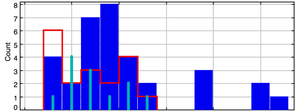
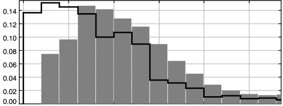
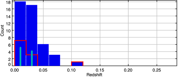
Figure 4: Redshift distributions. The $[\mathrm{Fe}\,\mbox{{x}}]$-selected sample (top) is subdivided by spectral type: broad blue bars represent broad-line Seyferts including all intermediate types (Sy1.0–1.9), narrow light blue spikes depict the NLS1s, and red outlines indicate the distribution of Seyfert 2.0s. For comparison, we present broader samples drawn from the SDSS-DR6 (middle): all $\sim$600,000 galaxies and quasars with $z<0.28$, and the 1098 $[\mathrm{O}\,\mbox{{i}}]$-emitting sources that satisfy criteria (i) through (iv) of §2 (grey filled-in histogram and black outline, respectively, with a normalized scale). The 65 NTM00 sources with reported $[\mathrm{Fe}\,\mbox{{x}}]$/$[\mathrm{O}\,\mbox{{iii}}]$ and $[\mathrm{Fe}\,\mbox{{vii}}]$/$[\mathrm{O}\,\mbox{{iii}}]$ ratios (bottom) are subdivided between BLS1s, NLS1s and Sy2s with the same symbols as the $[\mathrm{Fe}\,\mbox{{x}}]$ sample.

4.2 Line strengths

The distribution of $[\mathrm{O}\,\mbox{{iii}}]_{T}$ luminosities ($L_{[\mathrm{O}\,\mbox{{iii}}]_{T}}$) is similar amongst the BLS1s, NLS1s, and Sy2s in the $[\mathrm{Fe}\,\mbox{{x}}]$-selected SDSS sample (Fig. 5, top). The only clear difference is that the BLS1s extend to higher $L_{[\mathrm{O}\,\mbox{{iii}}]_{T}}$; these correspond to the highest-redshift members of the sample. The distributions of NTM00 are comparable except that a few of their lowest-redshift objects are found at considerably lower $L_{[\mathrm{O}\,\mbox{{iii}}]}$ values (Fig. 5, bottom). Thus, apart from a few sources at the extremes of the redshift distributions, the $[\mathrm{O}\,\mbox{{iii}}]$ power is reasonably well matched between the SDSS sample members of different spectral types and between the SDSS and NTM00 samples.

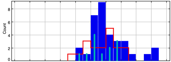
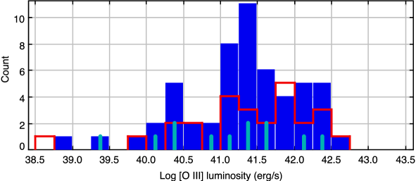
Figure 5: Distributions of $[\mathrm{O}\,\mbox{{iii}}]$ luminosities amongst BLS1s NLS1s, and Sy2s (symbols as in Fig. 4, top). The upper panel includes $[\mathrm{O}\,\mbox{{iii}}]_{T}$ luminosities for the 63 SDSS sample members; the lower panel presents the distributions for the 92 NTM00 objects with reported $[\mathrm{O}\,\mbox{{iii}}]$ luminosities. These luminosities have been re-evaluated using WMAP cosmological parameters.

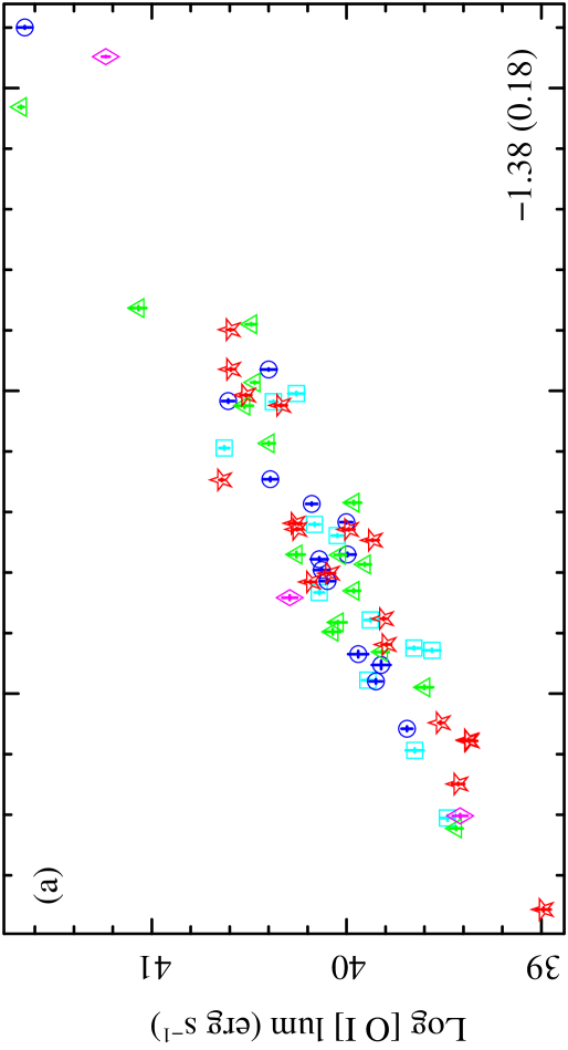
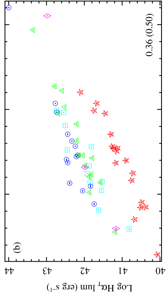
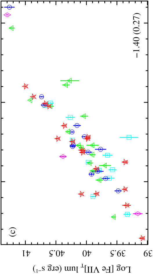
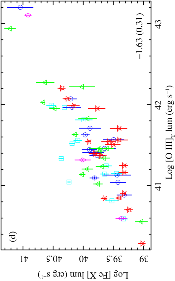
Figure 16: Luminosities of (a) $[\mathrm{O}\,\mbox{{i}}]$, (b) $\mathrm{H}\alpha_{T}$, (c) $[\mathrm{Fe}\,\mbox{{vii}}]_{T}$, and (d) $[\mathrm{Fe}\,\mbox{{x}}]$ vs. $[\mathrm{O}\,\mbox{{iii}}]_{T}$. Spectral classifications are indicated as in Fig. 15 and the numbers are again the mean of the logarithmic ratios (this time over $[\mathrm{O}\,\mbox{{iii}}]_{T}$) and the RMS about this average (in parenthesis).

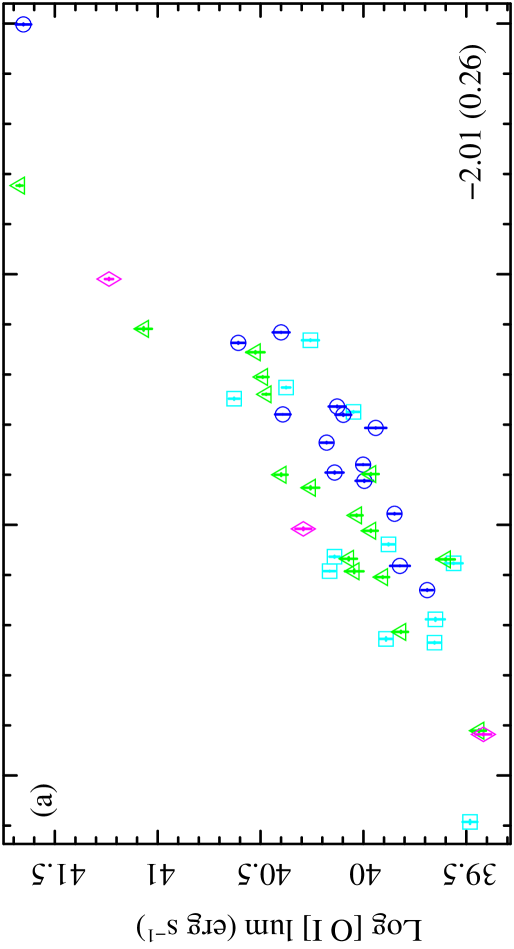
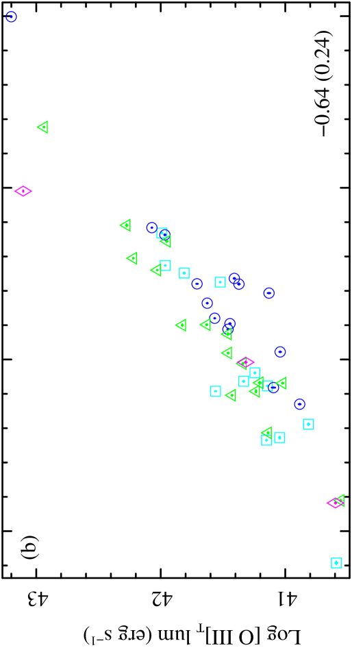
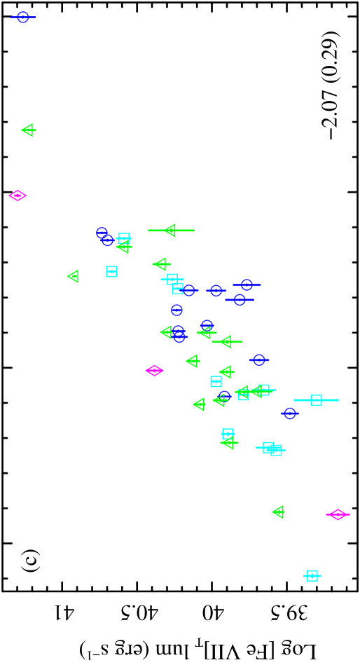
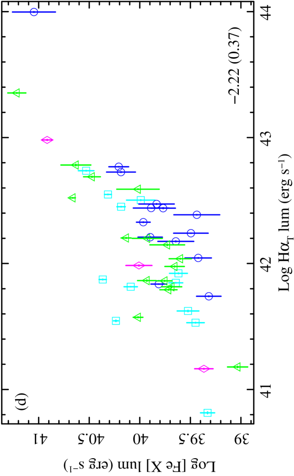
Figure 17: Luminosities of (a) $[\mathrm{O}\,\mbox{{i}}]$, (b) $[\mathrm{O}\,\mbox{{iii}}]_{T}$, (c) $[\mathrm{Fe}\,\mbox{{vii}}]_{T}$, and (d) $[\mathrm{Fe}\,\mbox{{x}}]$ vs. $\mathrm{H}\alpha_{T}$. Sy2 sources are omitted because their $\mathrm{H}\alpha_{T}$ luminosities are systematically lower because the broad component is not detected (see, e.g., Fig. 16b). Apart from the lack of Sy2s, point styles identical to Fig. 15 and the numbers are again the mean of the logarithmic ratios (over $\mathrm{H}\alpha_{T}$) and the RMS about this average (in parenthesis).

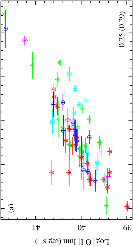
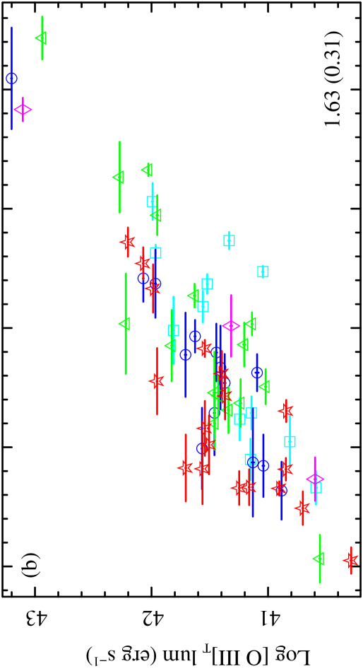
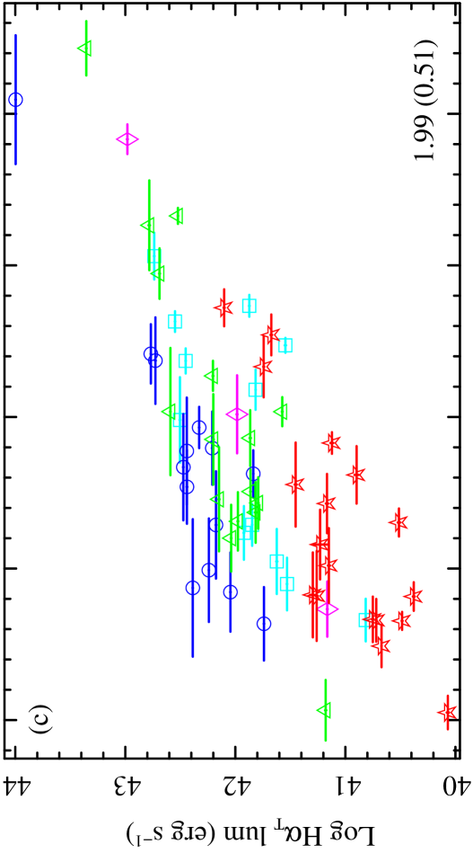
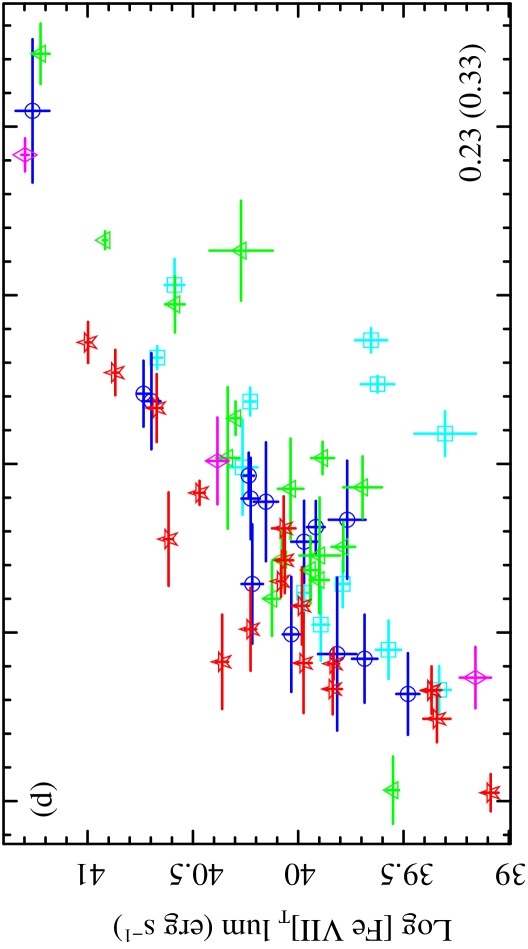
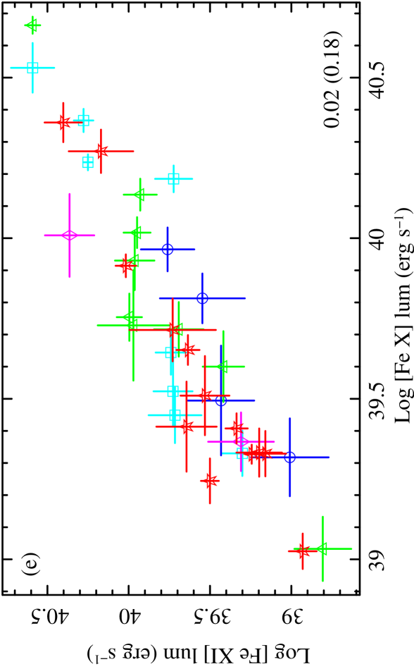
Figure 18: Luminosities of (a) $[\mathrm{O}\,\mbox{{i}}]$, (b) $[\mathrm{O}\,\mbox{{iii}}]_{T}$, (c) $\mathrm{H}\alpha_{T}$, (d) $[\mathrm{Fe}\,\mbox{{vii}}]_{T}$, and (e) $[\mathrm{Fe}\,\mbox{{xi}}]$ vs. $[\mathrm{Fe}\,\mbox{{x}}]$. Point styles as in Fig. 15 and the numbers are the mean of the logarithmic ratios (over $[\mathrm{Fe}\,\mbox{{x}}]$) and the RMS about this average (in parenthesis).

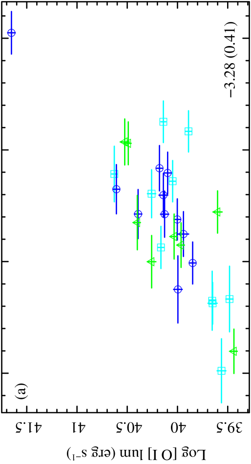
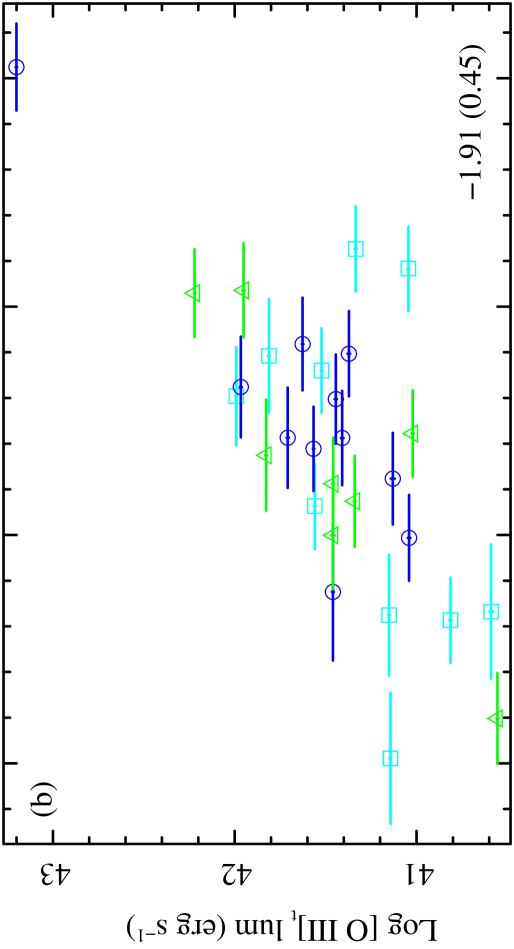
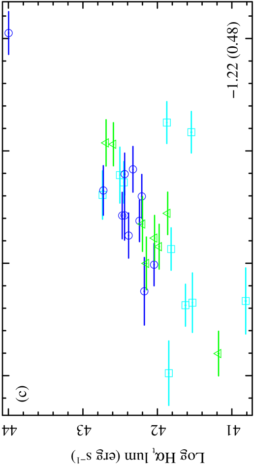
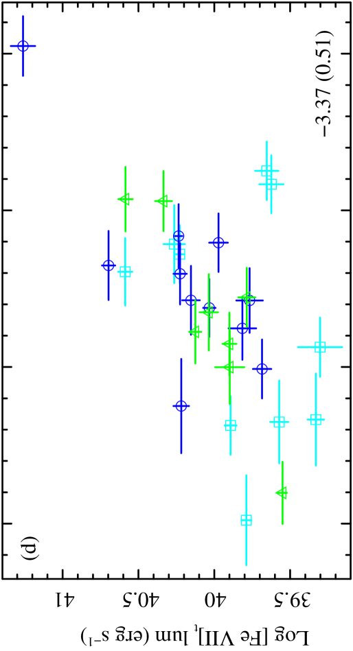
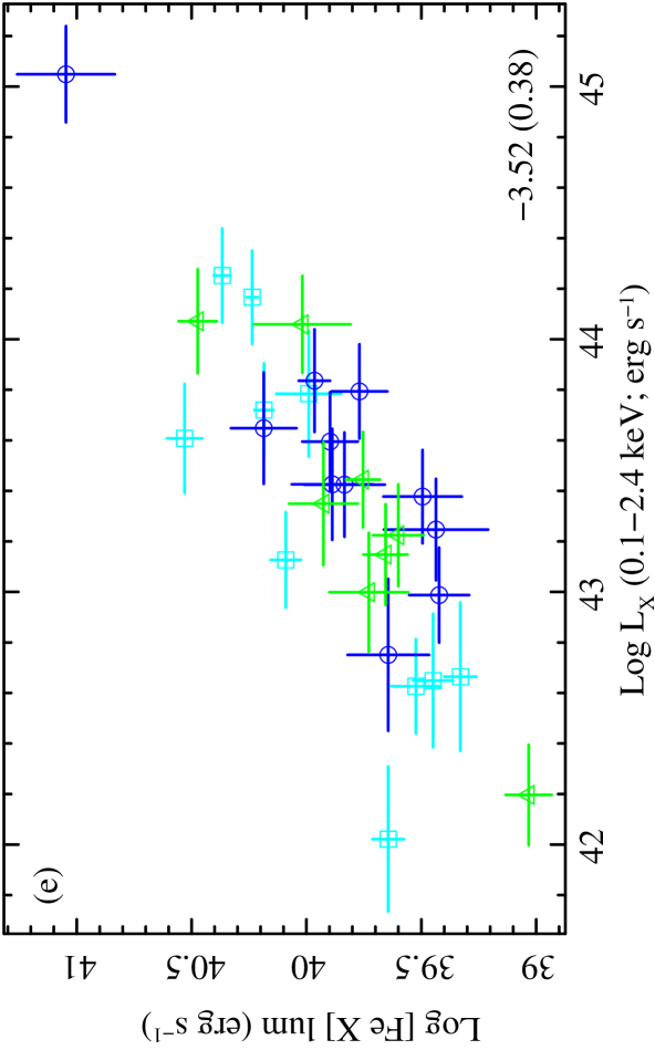
Figure 19: Luminosities of (a) $[\mathrm{O}\,\mbox{{i}}]$, (b) $[\mathrm{O}\,\mbox{{iii}}]_{T}$, (c) $\mathrm{H}\alpha_{T}$, (d) $[\mathrm{Fe}\,\mbox{{vii}}]_{T}$, and (e) $[\mathrm{Fe}\,\mbox{{x}}]$ vs. $L_{X}$ in the 0.1–2.4 keV band. Point styles as in Fig. 15 and the numbers are again the mean of the logarithmic ratios (over $F_{x}$) and the RMS about this average. The three Sy2s with Rosat detections are omitted because they are likely to be affected by X-ray absorption.

In Table 3 we present the correlation statistics between the fluxes of selected lines, line components, and the X-ray band (scatter plots demonstrating many of these correlations are provided online in Figs. 15–19). We find that all fluxes are positively correlated. This is to be expected because in general the more powerful AGN should be stronger emitters of both X-ray continuum and various lines. The more interesting questions to ask are which parameters correlate most strongly, with the least scatter, and whether any trends are present when ratios are used to normalize fluxes. These are summarized in Table 4, in which the average flux ratios and the RMS about each average are presented for the same pairs of fluxes appearing in Table 3.

Table 3: Correlation statistics amongst selected line and X-ray fluxes.

	$[\mathrm{O}\,\mbox{{i}}]$	$\mathrm{H}\alpha_{N}$	$\mathrm{H}\alpha_{T}$a	$[\mathrm{O}\,\mbox{{iii}}]_{T}$	$[\mathrm{Fe}\,\mbox{{vii}}]_{T}$	$[\mathrm{Fe}\,\mbox{{x}}]$	$[\mathrm{Fe}\,\mbox{{xi}}]$b	${F_{x}}^{c}$
$[\mathrm{O}\,\mbox{{i}}]$	—	0.760 (-12.2)	0.760 (-8.9)	0.856 (-18.4)	0.739 (-11.3)	0.650 (-8.1)	0.590 (-3.8)	0.603 (-3.3)
$\mathrm{H}\alpha_{N}$	0.760 (-12.2)	—	0.559 (-4.2)	0.752 (-11.9)	0.628 (-7.4)	0.659 (-8.4)	0.666 (-5.0)	0.539 (-2.6)
$\mathrm{H}\alpha_{T}$a	0.760 (-8.9)	0.559 (-4.2)	—	0.824 (-11.5)	0.748 (-8.4)	0.590 (-4.7)	0.640 (-3.0)	0.514 (-2.4)
$[\mathrm{O}\,\mbox{{iii}}]_{T}$	0.856 (-18.4)	0.752 (-11.9)	0.824 (-11.5)	—	0.820 (-15.7)	0.647 (-8.0)	0.587 (-3.8)	0.465 (-2.0)
$[\mathrm{Fe}\,\mbox{{vii}}]_{T}$	0.739 (-11.3)	0.628 (-7.4)	0.748 (-8.4)	0.820 (-15.7)	—	0.704 (-9.9)	0.617 (-4.2)	0.383 (-1.4)
$[\mathrm{Fe}\,\mbox{{x}}]$	0.650 (-8.1)	0.659 (-8.4)	0.590 (-4.7)	0.647 (-8.0)	0.704 (-9.9)	—	0.884 (-12.0)	0.646 (-3.8)
$[\mathrm{Fe}\,\mbox{{xi}}]$b	0.590 (-3.8)	0.666 (-5.0)	0.640 (-3.0)	0.587 (-3.8)	0.617 (-4.2)	0.884 (-12.0)	—	0.600 (-1.6)
${F_{x}}^{c}$	0.603 (-3.3)	0.539 (-2.6)	0.514 (-2.4)	0.465 (-2.0)	0.383 (-1.4)	0.646 (-3.8)	0.600 (-1.6)	—

^a $\mathrm{H}\alpha_{T}$ correlations include only the 45 type 1 Seyferts, as the Sy2s have only $\mathrm{H}\alpha_{N}$ components.

^b Only the 36 detections are used to evaluate most $[\mathrm{Fe}\,\mbox{{xi}}]$ correlations; 23 type 1 Seyferts are used for $\mathrm{H}\alpha_{T}$–$[\mathrm{Fe}\,\mbox{{xi}}]$, 14 for $F_{x}$–$[\mathrm{Fe}\,\mbox{{xi}}]$.

^c $F_{x}$ (0.1–2.4 keV) correlation statistics are based upon the 29 type 1 Seyferts with Rosat detections (14 sources in the case of $[\mathrm{Fe}\,\mbox{{xi}}]$).

Spearman rank correlation coefficient, $\rho$, and the log of the null hypothesis probability (i.e., the probability of finding by chance a correlation this strong between two parameters that are intrinsically not correlated; in parentheses) for selected emission line and X-ray fluxes. Probabilities are based upon the full sample of 63 objects unless noted otherwise. Values are repeated in the upper-right and lower-left halves of the table for convenience.

Table 4: Log of the average flux ratios, with RMS.

	$[\mathrm{O}\,\mbox{{i}}]$	$\mathrm{H}\alpha_{N}$	$\mathrm{H}\alpha_{T}$a	$[\mathrm{O}\,\mbox{{iii}}]_{T}$	$[\mathrm{Fe}\,\mbox{{vii}}]_{T}$	$[\mathrm{Fe}\,\mbox{{x}}]$	$[\mathrm{Fe}\,\mbox{{xi}}]$a	${F_{x}}^{a}$
$[\mathrm{O}\,\mbox{{i}}]$	—	1.00 (0.24)	2.01 (0.26)	1.38 (0.18)	-0.02 (0.30)	-0.25 (0.29)	-0.18 (0.34)	3.28 (0.41)
$\mathrm{H}\alpha_{N}$	-1.00 (0.24)	—	1.00 (0.36)	0.37 (0.24)	-1.02 (0.36)	-1.26 (0.31)	-1.19 (0.34)	2.33 (0.45)
$\mathrm{H}\alpha_{T}$a	-2.01 (0.26)	-1.00 (0.36)	—	-0.64 (0.24)	-2.07 (0.29)	-2.22 (0.37)	-2.08 (0.42)	1.22 (0.48)
$[\mathrm{O}\,\mbox{{iii}}]_{T}$	-1.38 (0.18)	-0.37 (0.24)	0.64 (0.24)	—	-1.40 (0.27)	-1.63 (0.31)	-1.54 (0.36)	1.91 (0.45)
$[\mathrm{Fe}\,\mbox{{vii}}]_{T}$	0.02 (0.30)	1.02 (0.36)	2.07 (0.29)	1.40 (0.27)	—	-0.23 (0.33)	-0.23 (0.37)	3.37 (0.51)
$[\mathrm{Fe}\,\mbox{{x}}]$	0.25 (0.29)	1.26 (0.31)	2.22 (0.37)	1.63 (0.31)	0.23 (0.33)	—	-0.02 (0.18)	3.52 (0.38)
$[\mathrm{Fe}\,\mbox{{xi}}]$a	0.18 (0.34)	1.19 (0.34)	2.08 (0.42)	1.54 (0.36)	0.23 (0.37)	0.02 (0.18)	—	3.43 (0.55)
${F_{x}}^{a}$	-3.28 (0.41)	-2.33 (0.45)	-1.22 (0.48)	-1.91 (0.45)	-3.37 (0.51)	-3.52 (0.38)	-3.43 (0.55)	—

^a As noted in Table 3, these ratios are based upon subsets of the $[\mathrm{Fe}\,\mbox{{x}}]$ sample: 45 type 1 Seyferts for ratios involving $\mathrm{H}\alpha_{T}$, the 29 type 1 Seyferts with X-ray detections for ratios involving $F_{x}$, and the 36 $[\mathrm{Fe}\,\mbox{{xi}}]$-detected sample members (of any spectral type) for the $[\mathrm{Fe}\,\mbox{{xi}}]$ ratios.

Log of the average flux ratios with RMS scatter about each mean (within parenthesis, reported in dex). Fluxes in the numerator are given across the top and those in the denominator are listed at the left. Thus, the entries in the first row are log($\mathrm{H}\alpha_{N}$/$[\mathrm{O}\,\mbox{{i}}]$), log($\mathrm{H}\alpha_{T}$/$[\mathrm{O}\,\mbox{{i}}]$), log($[\mathrm{O}\,\mbox{{iii}}]_{T}$/$[\mathrm{O}\,\mbox{{i}}]$), etc. Formal statistical uncertainties for the average ratios are $\pm 0.03$–0.05 for ratios defined by the full $[\mathrm{Fe}\,\mbox{{x}}]$ sample and can be as large as $\pm 0.10$ for ratios involving $[\mathrm{Fe}\,\mbox{{xi}}]$, $\mathrm{H}\alpha_{T}$, or $F_{x}$ due to the smaller subsamples upon which these are based (in the case of the $[\mathrm{Fe}\,\mbox{{xi}}]$/$F_{x}$ ratios, which involve only 14 data points, the uncertainty is $\pm 0.15$). Refer to the null hypothesis probabilities in Table 3 to assess whether these correlations are real.

Not unexpectedly, one of the best correlations, both in terms of strength (as measured by the Spearman rank correlation coefficient, $\rho$) and scatter (RMS about the mean ratio) is between $[\mathrm{Fe}\,\mbox{{x}}]$ and $[\mathrm{Fe}\,\mbox{{xi}}]$ (Fig. 6). The mean $[\mathrm{Fe}\,\mbox{{xi}}]$/$[\mathrm{Fe}\,\mbox{{x}}]$ ratio is $0.95\pm 0.08$ for the 36 sources in which we detect $[\mathrm{Fe}\,\mbox{{xi}}]$. Henceforth, we focus upon $[\mathrm{Fe}\,\mbox{{x}}]$ and not $[\mathrm{Fe}\,\mbox{{xi}}]$ when discussing the flux of the highest ionisation lines, as this line provides higher S/N, offers more detections, and is closer in wavelength to the other measured lines.

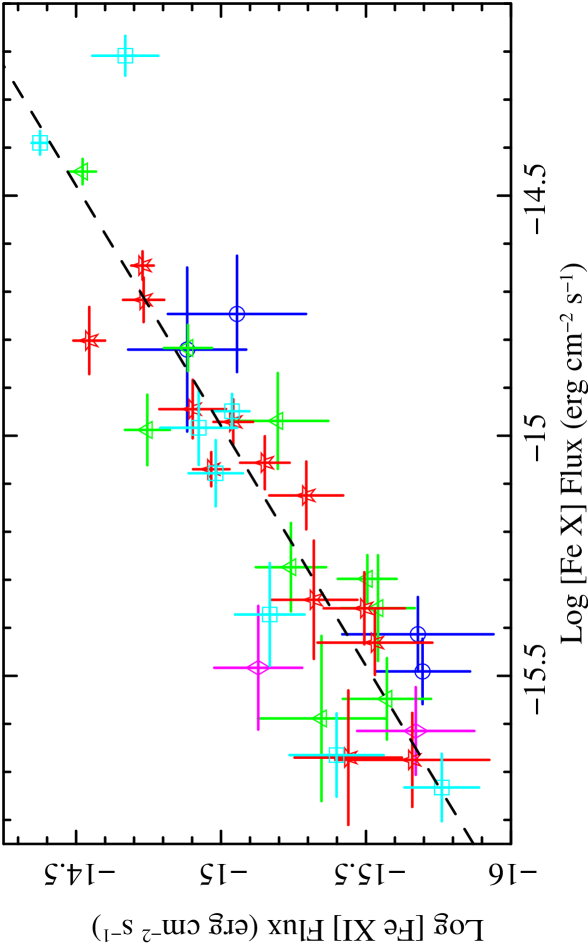
Figure 6: Fluxes of $[\mathrm{Fe}\,\mbox{{xi}}]$ and $[\mathrm{Fe}\,\mbox{{x}}]$. The dashed line represents the average $[\mathrm{Fe}\,\mbox{{xi}}]$/$[\mathrm{Fe}\,\mbox{{x}}]$ ratio, 0.95. Only two sample members have ratios that differ from this by $>2.3$-$\sigma$. Point styles are the same as in Fig. 3.

Apart from $[\mathrm{Fe}\,\mbox{{xi}}]$, the flux that correlates most strongly with $[\mathrm{Fe}\,\mbox{{x}}]$ is $[\mathrm{Fe}\,\mbox{{vii}}]_{T}$. The correlations with $[\mathrm{O}\,\mbox{{iii}}]_{T}$, $[\mathrm{O}\,\mbox{{iii}}]_{C}$, $\mathrm{H}\alpha_{N}$, and X-ray fluxes are comparable to each other and not much weaker than that with $[\mathrm{Fe}\,\mbox{{vii}}]_{T}$.

The next-highest ionisation species in this study is $[\mathrm{Fe}\,\mbox{{vii}}]$. Its ionisation potential is mid-way between those of $[\mathrm{Fe}\,\mbox{{x}}]$ and $[\mathrm{O}\,\mbox{{iii}}]$ (2.4$\times$ lower than the former and 2.8$\times$ higher than the latter), so it is unclear a priori whether $[\mathrm{Fe}\,\mbox{{vii}}]$ will have properties more like the higher-IP FHILs or the traditional NLR. As noted above, the flux of $[\mathrm{Fe}\,\mbox{{vii}}]_{T}$ correlates well with $[\mathrm{Fe}\,\mbox{{x}}]$. However, the strongest correlation and the smallest RMS scatter amongst the $[\mathrm{Fe}\,\mbox{{vii}}]_{T}$ flux ratios is provided by $[\mathrm{O}\,\mbox{{iii}}]_{T}$. We note that of the two $[\mathrm{O}\,\mbox{{iii}}]$ components, the flux of $[\mathrm{O}\,\mbox{{iii}}]_{W}$ is more closely correlated with $[\mathrm{Fe}\,\mbox{{vii}}]_{T}$, with $\rho=0.762$ and RMS = 0.29.

It is worth noting that when we use $[\mathrm{O}\,\mbox{{iii}}]_{T}$ strength to normalize $[\mathrm{Fe}\,\mbox{{vii}}]_{T}$, we do not find any significant differences between the NLS1, BLS1, and Sy2 populations (Fig. 7, top).

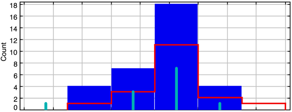
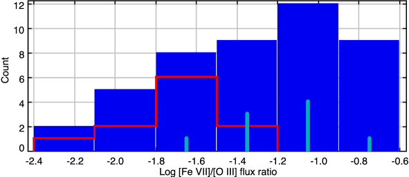
Figure 7: Distributions of $[\mathrm{Fe}\,\mbox{{vii}}]_{T}$/$[\mathrm{O}\,\mbox{{iii}}]_{T}$ flux ratios amongst NLS1, BLS1 and Sy2 populations in the $[\mathrm{Fe}\,\mbox{{x}}]$-selected and NTM00 samples (upper and lower panels, respectively). In contract with NTM00, we find no significant difference between the BLS1 and Sy2 distributions.

This contradicts MT98 and NTM00, who find that Seyfert 2s have substantially lower $[\mathrm{Fe}\,\mbox{{vii}}]$/$[\mathrm{O}\,\mbox{{iii}}]$ ratios (Fig. 7, bottom). In addition, NTM00 report a similar, albeit weaker, disparity in the distributions of $[\mathrm{Fe}\,\mbox{{x}}]$/$[\mathrm{O}\,\mbox{{iii}}]$ ratios between type 1 and type 2 Seyferts. Our $[\mathrm{Fe}\,\mbox{{x}}]$ data show something qualitatively similar, in that the $[\mathrm{Fe}\,\mbox{{x}}]$/$[\mathrm{O}\,\mbox{{iii}}]$ ratios of Sy2s tend to be lower than those of Sy1s, but quantitatively the difference we find is neither as large nor as significant as that reported by NTM00. These conflicting results are likely a consequence of how the samples are selected. The earlier studies used heterogeneous collections of nearby, well-known Seyferts with data drawn from the literature. In particular, 31 out of 65 sources for which NTM00 report both $[\mathrm{Fe}\,\mbox{{x}}]$/$[\mathrm{O}\,\mbox{{i}}]$ and $[\mathrm{Fe}\,\mbox{{vii}}]$/$[\mathrm{O}\,\mbox{{i}}]$ ratios have lower redshifts than any member of the SDSS $[\mathrm{Fe}\,\mbox{{x}}]$ sample (Fig. 4, bottom). This contrast is most pronounced for the obscured Seyferts: 18 out of 28 Sy1.9 and Sy2s are closer than any of the SDSS sources. As a result of this proximity and consequently the larger angular scale of the galactic structures, the observers may have been better able to isolate the unresolved nuclear emission from the extended flux. Thus the contamination due to stellar light may be reduced, allowing for the discovery of weaker nuclear features in a subset of their sample. Additionally, the area integrated might not have covered the full extent of the NLR, thereby affecting the observed flux ratios in some systems. The $[\mathrm{Fe}\,\mbox{{x}}]$-selected sample is more homogeneous, but our selection by $[\mathrm{Fe}\,\mbox{{x}}]$ creates a bias favoring sources with generally strong FHIL emission, reducing our sensitivity to low $[\mathrm{Fe}\,\mbox{{vii}}]_{T}$/$[\mathrm{O}\,\mbox{{iii}}]$ ratios as well as $[\mathrm{Fe}\,\mbox{{x}}]$-weak spectra. Moreover, we note that 38 per cent of the $[\mathrm{Fe}\,\mbox{{vii}}]$-detected sources in the NTM00 sample do not have $[\mathrm{Fe}\,\mbox{{x}}]$ detections. It is possible that there is a significant population of $[\mathrm{Fe}\,\mbox{{x}}]$-weak Seyferts that are missing from the present sample.

For the overall sample, the next-best $[\mathrm{Fe}\,\mbox{{vii}}]_{T}$ correlation after $[\mathrm{O}\,\mbox{{iii}}]$ is with $[\mathrm{Fe}\,\mbox{{x}}]$ (Fig. 8). However, we find that there is a systematic offset in this plane between the NLS1s and the Sy2s. Comparing linear regressions fitted to these two subsamples, we find that the $[\mathrm{Fe}\,\mbox{{x}}]$/$[\mathrm{Fe}\,\mbox{{vii}}]_{T}$ ratios of NLS1s tend to be 2–3 times higher. Whilst the line fitted to the NLS1s is influenced by a few notable outliers and there is some overlap between these subsamples, not one NLS1 lies below the line fitted to the Sy2s (red dashed line). Table 3 shows that $[\mathrm{Fe}\,\mbox{{vii}}]_{T}$ also correlates very well with $\mathrm{H}\alpha_{T}$, but this is only true when Sy2s are excluded from the analysis ($\mathrm{H}\alpha_{T}$ is dominated by $\mathrm{H}\alpha_{B}$ in the type 1 Seyferts, whereas by definition the $\mathrm{H}\alpha$ lines in Sy2s do not have any BLR contribution; Fig. 17c). The weakest $[\mathrm{Fe}\,\mbox{{vii}}]$ correlation and the worst scatter is provided by X-ray flux (Fig. 19d), in contrast to the case of $[\mathrm{Fe}\,\mbox{{x}}]$ and X-rays.

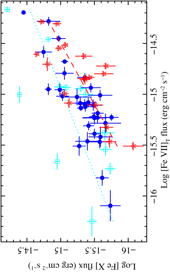
Figure 8: $[\mathrm{Fe}\,\mbox{{x}}]$ vs. $[\mathrm{Fe}\,\mbox{{vii}}]_{T}$ flux. Blue filled circles are BLS1s (Sy1.0, 1.5 and 1.9), cyan open squares are NLS1s, and red stars are Sy2s; the cyan dotted line is a linear regression fitted to the NLS1s and the red dashed line is a line fitted to the Sy2s. The distribution of NLS1s and Sy2s overlap, but the $[\mathrm{Fe}\,\mbox{{x}}]$/$[\mathrm{Fe}\,\mbox{{vii}}]_{T}$ ratios of the NLS1s are systematically higher than those of the Sy2s: not one NLS1 lies below the line fitted to the Sy2s.

The most prominent of the lower-ionisation forbidden lines is $[\mathrm{O}\,\mbox{{iii}}]$. The $[\mathrm{O}\,\mbox{{iii}}]_{T}$ flux correlates well with all of the other lines with $\mathrm{IP}<100$ eV ($\rho\geq 0.75$). However, it is $[\mathrm{O}\,\mbox{{i}}]$ that correlates best when all spectral types are considered, followed by $[\mathrm{Fe}\,\mbox{{vii}}]_{T}$. When we consider only the type 1 Seyferts, we find that $[\mathrm{O}\,\mbox{{iii}}]_{T}$ correlates comparably well with $\mathrm{H}\alpha_{T}$ as with $[\mathrm{O}\,\mbox{{i}}]$ and $[\mathrm{Fe}\,\mbox{{vii}}]_{T}$ ($\rho=0.82$, 0.82, and 0.80, respectively).

4.3 Line profiles

The widths and velocity shifts ($v_{\mathrm{sh}}$) of the best-fitting line components are summarized in Table 5 for both the overall sample and subsets defined by Seyfert spectral classification. Note that $[\mathrm{Fe}\,\mbox{{xi}}]$ and $[\mathrm{Fe}\,\mbox{{vii}}]_{W}$ are included in only some of final models. Consequently, the values of these parameters are more strongly affected by small number statistics, especially for some subsamples, and should be interpreted with caution. Likewise, there are only three Sy1.9s so the typical line properties of this class of Seyfert are not very well constrained; their average best-fitting parameters have large uncertainties and are consistent with those of both the Sy1.5s and the 2.0s. We therefore exclude Sy1.9s from Table 5. Caution is also advised when comparing lines fitted with different models, as this can introduce systematic effects. To facilitate the comparison of $[\mathrm{Fe}\,\mbox{{vii}}]$ with higher-ionisation FHILs, we include statistics for the best-fitting single-Gaussian models, $[\mathrm{Fe}\,\mbox{{vii}}]_{1G}$, as well as the double-Gaussian components.

Table 5: Average parameters of fitted line profiles.

Line	Overall	NLS1	Sy1.0	Sy1.5	Sy2
model	Mean (RMS)	Mean (RMS)	Mean (RMS)	Mean (RMS)	Mean (RMS)
Line velocities measured relative to $[\mathrm{S}\,\mbox{{ii}}]$ ($v_{\mathrm{sh}}$, $\mathrm{km\,s^{-1}}$)
$[\mathrm{O}\,\mbox{{iii}}]_{C}$	-5 $\pm$ 5 (40)	-8 $\pm$ 6 (21)	-8 $\pm$ 6 (22)	-15 $\pm$ 13 (50)	12 $\pm$ 11 (47)
$[\mathrm{O}\,\mbox{{iii}}]_{W}$	-134 $\pm$ 19 (147)	-112 $\pm$ 30 (100)	-65 $\pm$ 24 (87)	-134 $\pm$ 57 (221)	-196 $\pm$ 29 (121)
$[\mathrm{O}\,\mbox{{i}}]$	0 $\pm$ 4 (30)	7 $\pm$ 7 (23)	-1 $\pm$ 6 (20)	-2 $\pm$ 12 (46)	2 $\pm$ 5 (21)
$[\mathrm{Fe}\,\mbox{{vii}}]_{C}$	-74 $\pm$ 16 (128)	-99 $\pm$ 41 (136)	-54 $\pm$ 28 (101)	-93 $\pm$ 42 (163)	-44 $\pm$ 25 (103)
$[\mathrm{Fe}\,\mbox{{vii}}]_{W}$a	-296 $\pm$ 28 (102)	-331 $\pm$ — (—)	-213 $\pm$ 63 (63)	-305 $\pm$ 63 (63)	-308 $\pm$ 42 (118)
$[\mathrm{Fe}\,\mbox{{vii}}]_{1G}$	-86 $\pm$ 16 (126)	-100 $\pm$ 41 (135)	-57 $\pm$ 27 (99)	-95 $\pm$ 42 (162)	-83 $\pm$ 25 (102)
$[\mathrm{Fe}\,\mbox{{x}}]$	-84 $\pm$ 18 (143)	-128 $\pm$ 44 (147)	-39 $\pm$ 36 (130)	-107 $\pm$ 44 (171)	-61 $\pm$ 30 (124)
$[\mathrm{Fe}\,\mbox{{xi}}]$a	-212 $\pm$ 32 (192)	-258 $\pm$ 39 (103)	-41 $\pm$ 19 (33)	-217 $\pm$ 76 (216)	-186 $\pm$ 52 (181)
$\mathrm{H}\alpha_{N}$	-34 $\pm$ 11 (85)	-69 $\pm$ 21 (68)	-27 $\pm$ 33 (120)	-32 $\pm$ 24 (93)	-22 $\pm$ 13 (52)
$\mathrm{H}\alpha_{B}$	-3 $\pm$ 26 (206)	52 $\pm$ 21 (71)	-6 $\pm$ 70 (253)	24 $\pm$ 57 (222)	—
Line widths (FWHM; $\mathrm{km\,s^{-1}}$)
$[\mathrm{S}\,\mbox{{ii}}]$	322 $\pm$ 12 (90)	284 $\pm$ 22 (73)	314 $\pm$ 24 (88)	330 $\pm$ 25 (98)	346 $\pm$ 23 (90)
$[\mathrm{O}\,\mbox{{iii}}]_{C}$	319 $\pm$ 12 (96)	267 $\pm$ 14 (48)	315 $\pm$ 17 (63)	363 $\pm$ 36 (140)	316 $\pm$ 19 (80)
$[\mathrm{O}\,\mbox{{iii}}]_{W}$	779 $\pm$ 33 (257)	801 $\pm$ 59 (196)	758 $\pm$ 48 (175)	777 $\pm$ 77 (298)	798 $\pm$ 72 (296)
$[\mathrm{O}\,\mbox{{i}}]$	380 $\pm$ 20 (154)	299 $\pm$ 21 (70)	354 $\pm$ 19 (70)	437 $\pm$ 55 (213)	404 $\pm$ 41 (169)
$[\mathrm{Fe}\,\mbox{{vii}}]_{C}$	500 $\pm$ 29 (230)	502 $\pm$ 74 (245)	489 $\pm$ 53 (190)	561 $\pm$ 60 (234)	433 $\pm$ 57 (236)
$[\mathrm{Fe}\,\mbox{{vii}}]_{W}$a	860 $\pm$ 91 (327)	652 $\pm$ — (—)	696 $\pm$ 357 (357)	459 $\pm$ 279 (279)	1009 $\pm$ 94 (267)
$[\mathrm{Fe}\,\mbox{{vii}}]_{1G}$	571 $\pm$ 29 (230)	507 $\pm$ 73 (241)	526 $\pm$ 43 (156)	567 $\pm$ 59 (227)	645 $\pm$ 64 (263)
$[\mathrm{Fe}\,\mbox{{x}}]$	556 $\pm$ 32 (251)	591 $\pm$ 73 (241)	508 $\pm$ 35 (125)	690 $\pm$ 84 (326)	447 $\pm$ 56 (231)
$[\mathrm{Fe}\,\mbox{{xi}}]$a	643 $\pm$ 65 (383)	864 $\pm$ 176 (467)	463 $\pm$ 104 (180)	749 $\pm$ 161 (455)	488 $\pm$ 78 (272)
$\mathrm{H}\alpha_{N}$	415 $\pm$ 20 (157)	335 $\pm$ 29 (95)	405 $\pm$ 25 (91)	498 $\pm$ 57 (219)	406 $\pm$ 35 (143)
$\mathrm{H}\alpha_{B}$	3475 $\pm$ 273 (1949)	1515 $\pm$ 150 (498)	4718 $\pm$ 523 (1887)	4491 $\pm$ 377 (1458)	—
Model counts
Most features	63	12	14	16	18
$[\mathrm{Fe}\,\mbox{{vii}}]_{W}$	14	1	2	2	9
$[\mathrm{Fe}\,\mbox{{xi}}]$	36	8	4	9	13
a Statistics are limited (especially for some spectral types) because not all final models include $[\mathrm{Fe}\,\mbox{{vii}}]_{W}$ and $[\mathrm{Fe}\,\mbox{{xi}}]$.

Forbidden lines are listed in order of increasing $N_{cr}$. Columns are: (1) Line model component; (2–6) average value $\pm$ the 1-$\sigma$ statistical uncertainty of mean and the RMS distribution (in parentheses) of model parameters for overall sample and subsets of each spectral type: (2) all Seyfert types, including Sy1.9s; (3) NLS1; (4) Sy1.0; (5) Sy1.5; (6) Sy2. Sy1.9s are not presented because there are only three in our sample (two with detected $[\mathrm{Fe}\,\mbox{{xi}}]$, none with $[\mathrm{Fe}\,\mbox{{vii}}]_{W}$), so the average model parameters are not very well constrained. The Sy1.9 averages are consistent with those of both Sy1.5s and Sy2s.

Several things may be demonstrated with the average profile properties in Table 5. We find that the cores of lines with the lowest IPs have velocity shifts that are generally consistent with $[\mathrm{S}\,\mbox{{ii}}]$, whilst the wings of $[\mathrm{O}\,\mbox{{iii}}]$ tend to be outflowing. The $[\mathrm{Fe}\,\mbox{{vii}}]$ profiles are characterized by blue cores and sometimes include even bluer wings. The most blueshifted lines are found in our highest IP feature, $[\mathrm{Fe}\,\mbox{{xi}}]$. The widths of the line cores and single-Gaussian line models increase monotonically with critical density, with $[\mathrm{Fe}\,\mbox{{xi}}]$ exhibiting the broadest lines. Thus, we reaffirm earlier studies that found a tendency for the line width and blue shifts to increase with increasing IP (e.g., Appenzeller & Öestreicher, 1988). Moreover, the FHIL profiles are quantitatively similar to previous results. According to Erkens et al. (1997) the average FWHM ratios of the FHILs over $[\mathrm{O}\,\mbox{{iii}}]$ are 1.63, 1.58 and 1.86 respectively for the $[\mathrm{Fe}\,\mbox{{vii}}]$/$[\mathrm{O}\,\mbox{{iii}}]$, $[\mathrm{Fe}\,\mbox{{x}}]$/$[\mathrm{O}\,\mbox{{iii}}]$ and $[\mathrm{Fe}\,\mbox{{xi}}]$/$[\mathrm{O}\,\mbox{{iii}}]$ width ratios; we obtain values of 1.60, 1.60 and 2.04 for the width ratios of $[\mathrm{Fe}\,\mbox{{vii}}]_{1G}$, $[\mathrm{Fe}\,\mbox{{x}}]$ and $[\mathrm{Fe}\,\mbox{{xi}}]$ over $[\mathrm{O}\,\mbox{{i}}]$ (here we use $[\mathrm{Fe}\,\mbox{{vii}}]_{1G}$ and $[\mathrm{O}\,\mbox{{i}}]$ instead of $[\mathrm{Fe}\,\mbox{{vii}}]_{C}$ and $[\mathrm{O}\,\mbox{{iii}}]_{C}$ to be consistent in using single-Gaussian models). Comparing the different Seyfert types, we find that the NLS1s tend to have the highest FHIL outflow velocities, whilst the Sy2s tend to have the narrowest FHILs.

In Table 6 we present the correlation statistics between the line profile parameters of various emission features. These statistics show that the velocity shift correlations between the FHILs are universally stronger than those between any other pair of features. On the other hand, with the exception of the $[\mathrm{Fe}\,\mbox{{xi}}]$–$[\mathrm{Fe}\,\mbox{{x}}]$ pair, the strongest line width correlations are found amongst the low-IP features.

Table 6: Correlation statistics the line profile parameters of selected emission lines.

Line $v_{\mathrm{sh}}$ correlation statistics
	$[\mathrm{O}\,\mbox{{i}}]$	$\mathrm{H}\alpha_{N}$	$[\mathrm{O}\,\mbox{{iii}}]_{C}$	$[\mathrm{O}\,\mbox{{iii}}]_{W}$	$[\mathrm{Fe}\,\mbox{{vii}}]_{1G}$	$[\mathrm{Fe}\,\mbox{{vii}}]_{C}$	$[\mathrm{Fe}\,\mbox{{x}}]$	$[\mathrm{Fe}\,\mbox{{xi}}]$
$[\mathrm{O}\,\mbox{{i}}]$	—	—	0.621 (-7.2)	0.469 (-4.0)	0.390 (-2.8)	0.318 (-2.0)	0.330 (-2.1)	0.508 (-2.8)
$\mathrm{H}\alpha_{N}$	—	—	0.321 (-2.0)	0.162 (-0.7)	0.315 (-1.9)	0.344 (-2.2)	0.341 (-2.2)	0.156 (-0.4)
$[\mathrm{O}\,\mbox{{iii}}]_{C}$	0.621 (-7.2)	0.321 (-2.0)	—	0.237 (-1.2)	0.445 (-3.6)	0.473 (-4.0)	0.302 (-1.8)	0.397 (-1.8)
$[\mathrm{O}\,\mbox{{iii}}]_{W}$	0.469 (-4.0)	0.162 (-0.7)	0.237 (-1.2)	—	0.367 (-2.5)	0.255 (-1.4)	0.308 (-1.9)	0.391 (-1.7)
$[\mathrm{Fe}\,\mbox{{vii}}]_{1G}$	0.390 (-2.8)	0.315 (-1.9)	0.445 (-3.6)	0.367 (-2.5)	—	—	0.681 (-9.1)	0.754 (-7.0)
$[\mathrm{Fe}\,\mbox{{vii}}]_{C}$	0.318 (-2.0)	0.344 (-2.2)	0.473 (-4.0)	0.255 (-1.4)	—	—	0.697 (-9.7)	0.702 (-5.7)
$[\mathrm{Fe}\,\mbox{{x}}]$	0.330 (-2.1)	0.341 (-2.2)	0.302 (-1.8)	0.308 (-1.9)	0.681 (-9.1)	0.697 (-9.7)	—	0.761 (-7.1)
$[\mathrm{Fe}\,\mbox{{xi}}]$	0.508 (-2.8)	0.156 (-0.4)	0.397 (-1.8)	0.391 (-1.7)	0.754 (-7.0)	0.702 (-5.7)	0.761 (-7.1)	—
Line FWHM correlation statistics
	$[\mathrm{O}\,\mbox{{i}}]$	$\mathrm{H}\alpha_{N}$	$[\mathrm{O}\,\mbox{{iii}}]_{C}$	$[\mathrm{O}\,\mbox{{iii}}]_{W}$	$[\mathrm{Fe}\,\mbox{{vii}}]_{1G}$	$[\mathrm{Fe}\,\mbox{{vii}}]_{C}$	$[\mathrm{Fe}\,\mbox{{x}}]$	$[\mathrm{Fe}\,\mbox{{xi}}]$
$[\mathrm{O}\,\mbox{{i}}]$	—	—	0.810 (-15.1)	0.539 (-5.3)	0.460 (-3.8)	0.356 (-2.4)	0.163 (-0.7)	0.196 (-0.6)
$\mathrm{H}\alpha_{N}$	—	—	0.829 (-16.3)	0.567 (-5.9)	0.483 (-4.2)	0.352 (-2.3)	0.259 (-1.4)	0.331 (-1.3)
$[\mathrm{O}\,\mbox{{iii}}]_{C}$	0.810 (-15.1)	0.829 (-16.3)	—	0.693 (-9.5)	0.422 (-3.2)	0.242 (-1.3)	0.312 (-1.9)	0.332 (-1.3)
$[\mathrm{O}\,\mbox{{iii}}]_{W}$	0.539 (-5.3)	0.567 (-5.9)	0.693 (-9.5)	—	0.331 (-2.1)	0.047 (-0.1)	0.099 (-0.4)	0.132 (-0.4)
$[\mathrm{Fe}\,\mbox{{vii}}]_{1G}$	0.460 (-3.8)	0.483 (-4.2)	0.422 (-3.2)	0.331 (-2.1)	—	—	0.411 (-3.1)	0.605 (-4.0)
$[\mathrm{Fe}\,\mbox{{vii}}]_{C}$	0.356 (-2.4)	0.352 (-2.3)	0.242 (-1.3)	0.047 (-0.1)	—	—	0.457 (-3.8)	0.588 (-3.8)
$[\mathrm{Fe}\,\mbox{{x}}]$	0.163 (-0.7)	0.259 (-1.4)	0.312 (-1.9)	0.099 (-0.4)	0.411 (-3.1)	0.457 (-3.8)	—	0.773 (-7.5)
$[\mathrm{Fe}\,\mbox{{xi}}]$	0.196 (-0.6)	0.331 (-1.3)	0.332 (-1.3)	0.132 (-0.4)	0.605 (-4.0)	0.588 (-3.8)	0.773 (-7.5)	—

Spearman rank correlation coefficient ($\rho$) and the log of the null hypothesis probability (in parentheses) for the profile parameters of selected emission lines. Statistics are based upon the full $[\mathrm{Fe}\,\mbox{{x}}]$-selected sample with the exception of $[\mathrm{Fe}\,\mbox{{xi}}]$ correlations, which use only the 36 $[\mathrm{Fe}\,\mbox{{xi}}]$ detections. $\mathrm{H}\alpha_{B}$ is omitted from the table because it was not found to correlate significantly with any of these parameters; its FWHM exhibits no correlations with confidence above the 90 per cent level, whilst its velocity showed no correlations with even 50 per cent confidence. $[\mathrm{Fe}\,\mbox{{vii}}]_{W}$ is omitted because it is only applied to 14 sample members so the confidence levels of its correlations are low; its only correlation found to have $>99$ per cent confidence is between the FWHM values of $[\mathrm{Fe}\,\mbox{{vii}}]_{W}$ and $[\mathrm{O}\,\mbox{{iii}}]_{W}$. We do not report correlations between the profiles of $[\mathrm{O}\,\mbox{{i}}]$ and $\mathrm{H}\alpha_{N}$ and between $[\mathrm{Fe}\,\mbox{{vii}}]_{1G}$ and $[\mathrm{Fe}\,\mbox{{vii}}]_{C}$ because these models are often constrained to have the same profiles; in particular these $[\mathrm{Fe}\,\mbox{{vii}}]$ models are identical in all but 14 instances. As with Table 3 the values are repeated in the upper-right and lower-left halves of these tables for convenience.

The profiles of $[\mathrm{Fe}\,\mbox{{x}}]$ and $[\mathrm{Fe}\,\mbox{{xi}}]$ are mutually consistent for much of the sample, but a subset of the $[\mathrm{Fe}\,\mbox{{xi}}]$ lines appear to be both broader and bluer (Fig. 9a–b). The velocity shifts are almost always negative, indicating that the emitting clouds are outflowing. The $v_{\mathrm{sh}}$ values are consistent for roughly half of the sample, whereas the $[\mathrm{Fe}\,\mbox{{xi}}]$ outflow velocities are significantly faster in roughly one third of the sources ($[\mathrm{Fe}\,\mbox{{xi}}]$ is faster in 11 out of 36 sources with at least 3-$\sigma$ confidence). In no instance is $[\mathrm{Fe}\,\mbox{{xi}}]$ significantly slower. Overall, the average velocity shift difference is $v_{\mathrm{sh}}\,([\mathrm{Fe}\,\mbox{{xi}}])-v_{\mathrm{sh}}\,([\mathrm{Fe}\,\mbox{{x}}])=-109\ \mathrm{km\,s^{-1}}$ with an RMS scatter of 126 $\mathrm{km\,s^{-1}}$. The widths of the $[\mathrm{Fe}\,\mbox{{xi}}]$ lines tend to be either consistent with or broader than $[\mathrm{Fe}\,\mbox{{x}}]$ (Fig. 9b), although the FWHM values are not as well constrained as $v_{\mathrm{sh}}$. For both ionic species, the fastest outflow velocities are found amongst the broadest lines (although the broadest lines do not always have fast $v_{\mathrm{sh}}$ values).

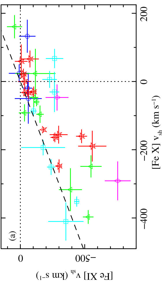
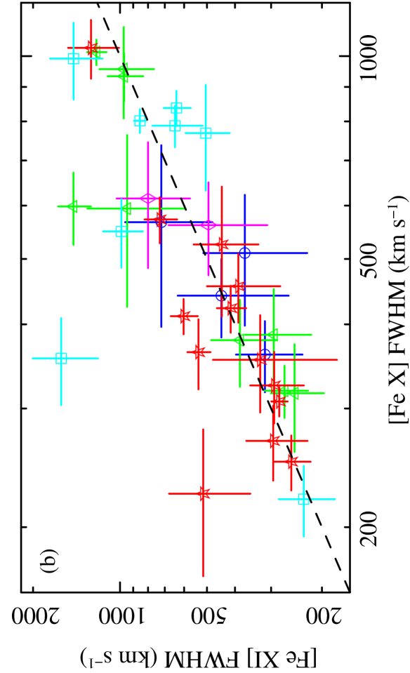
Figure 9: Velocity shifts (a) and FWHM (b) of $[\mathrm{Fe}\,\mbox{{xi}}]$ and $[\mathrm{Fe}\,\mbox{{x}}]$. Point shapes and colours are the same as Fig. 3. Dashed $x=y$ lines are included to guide the eye. Most $[\mathrm{Fe}\,\mbox{{x}}]$ and $[\mathrm{Fe}\,\mbox{{xi}}]$ lines appear to be outflowing ($v_{\mathrm{sh}}<0\ \mathrm{km\,s^{-1}}$). In a little more than half the sample the $v_{\mathrm{sh}}$ values are consistent; in the remaining cases the outflow velocities of $[\mathrm{Fe}\,\mbox{{xi}}]$ are faster (by up to 300 $\mathrm{km\,s^{-1}}$). The FWHM values of $[\mathrm{Fe}\,\mbox{{xi}}]$ tend to be either as broad or broader than those of $[\mathrm{Fe}\,\mbox{{x}}]$, but the line width uncertainties are large.

Unlike $[\mathrm{Fe}\,\mbox{{xi}}]$, there is no tendency for the $[\mathrm{Fe}\,\mbox{{vii}}]_{1G}$ models to have different widths or velocity shifts from those of $[\mathrm{Fe}\,\mbox{{x}}]$. The average velocity shift difference is effectively zero with somewhat less scatter ($v_{\mathrm{sh}}\,([\mathrm{Fe}\,\mbox{{x}}])-v_{\mathrm{sh}}\,([\mathrm{Fe}\,\mbox{{vii}}]_{1G})=5\ \mathrm{km\,s^{-1}}$ with $\mathrm{RMS}=108\ \mathrm{km\,s^{-1}}$). Likewise, there is no significant difference between the widths of $[\mathrm{Fe}\,\mbox{{vii}}]_{1G}$ and $[\mathrm{Fe}\,\mbox{{x}}]$. However, in contrast to $v_{\mathrm{sh}}$, the correlation of the line widths is weaker and lower confidence.

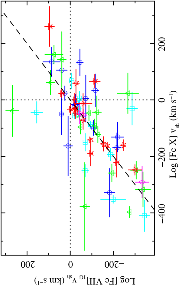
Figure 10: Velocity shifts of $[\mathrm{Fe}\,\mbox{{vii}}]_{1G}$ and $[\mathrm{Fe}\,\mbox{{x}}]$. A dashed $x=y$ line is sketched to guide the eye. Point shapes and colours are the same as Fig. 3. Unlike the $v_{\mathrm{sh}}$ values of $[\mathrm{Fe}\,\mbox{{xi}}]$ (Fig. 9a), there is no tendency for the $[\mathrm{Fe}\,\mbox{{vii}}]_{1G}$ lines to be more or less shifted than $[\mathrm{Fe}\,\mbox{{x}}]$. The scatter in this plot is dominated by a few data points with large $[\mathrm{Fe}\,\mbox{{x}}]$ $v_{\mathrm{sh}}$ uncertainties.

Amongst the lower-IP features, the only lines or line components that tend to be in outflow are the wings of $[\mathrm{O}\,\mbox{{iii}}]$. At best, the velocity shifts of $[\mathrm{O}\,\mbox{{iii}}]_{W}$ and the FHILs are weakly correlated (only $[\mathrm{Fe}\,\mbox{{vii}}]_{1G}$ appears to correlate with greater than 99 per cent confidence). However, as noted in §3.2.3, there is a degeneracy in the process of separating the core and wing component models that introduces additional uncertainties in these component parameters, possibly causing systematic effects and certainly increasing the noise. We therefore interpret the $[\mathrm{O}\,\mbox{{iii}}]_{W}$ parameters with caution. It is true that the measured $[\mathrm{O}\,\mbox{{iii}}]_{W}$ outflow velocities tend to be higher than those of $[\mathrm{Fe}\,\mbox{{vii}}]_{C}$, $[\mathrm{Fe}\,\mbox{{vii}}]_{1G}$ and $[\mathrm{Fe}\,\mbox{{x}}]$, but this may be an artefact of the deblending process. What is clear is that $[\mathrm{O}\,\mbox{{iii}}]$ has (at least) two components, the broader of which is outflowing whilst the narrower one is not shifted relative to the lower-ionisation species such as $[\mathrm{S}\,\mbox{{ii}}]$ and $[\mathrm{O}\,\mbox{{i}}]$. The fact that the measured $[\mathrm{O}\,\mbox{{iii}}]_{W}$ velocity shifts are not much larger than those of the FHILs leaves open the possibility that this component may be kinematically related to the FHIL-emitting region.

4.4 X-ray properties

In Fig. 11, we show the correlation between $[\mathrm{Fe}\,\mbox{{x}}]$ and 0.1–2.4 keV fluxes amongst the 32 sample members with Rosat detections. The $[\mathrm{Fe}\,\mbox{{x}}]$ intensities of the type 1 Seyferts (1.0, 1.5 & NLS1) scale with power in the X-ray band, consistent with the trend shown by Porquet et al. (1999, fig. 2; represented here in Fig. 11 by the diagonal dashed line). The only three Rosat-detected Seyfert 2s have by far the highest $[\mathrm{Fe}\,\mbox{{x}}]$/X-ray ratios, by roughly a factor of 30 over the type 1 Seyferts. Moreover, as demonstrated by the plot of $[\mathrm{Fe}\,\mbox{{x}}]$ and X-ray luminosities (Fig. 12, upper panel) they also have some of the lowest observed X-ray powers. This is readily interpreted within the Seyfert unification framework (e.g., Antonucci, 1993) as obscuration along the line of sight to the X-ray emitting regions of the type 2 systems. If such obscuration also affects our view of the FHIL-emitting clouds, then it must cover only a fraction of this region as these sources are detected by their $[\mathrm{Fe}\,\mbox{{x}}]$ lines.

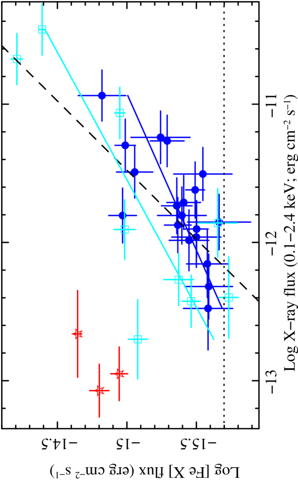
Figure 11: $[\mathrm{Fe}\,\mbox{{x}}]$ vs. X-ray flux in the full Rosat band (0.1–2.4 keV). Point styles are the same as in Fig. 8. The solid diagonal lines are linear correlations fitted to the NLS1 (higher, cyan line) and BLS1 (lower, blue line) populations. The horizontal dotted line at $F_{[\mathrm{Fe}\,\mbox{{x}}]}=2\times 10^{-16}\ \mathrm{erg\,cm^{-2}\,s^{-1}}$ is the approximate flux limit of $[\mathrm{Fe}\,\mbox{{x}}]$ in our sample. The black dashed line indicates a constant ratio of $[\mathrm{Fe}\,\mbox{{x}}]/\mbox{X-ray}=3\times 10^{-4}$, which is representative of the flux ratios shown by Porquet et al. (1999). Apart from the Seyfert 2s, which are likely affected by X-ray absorption, the highest $[\mathrm{Fe}\,\mbox{{x}}]$/X-ray ratios are generally NLS1s.

The lower IP lines do not correlate as tightly with X-ray power. This is illustrated by Fig. 12, which plots the luminosities of $[\mathrm{Fe}\,\mbox{{x}}]$, $[\mathrm{O}\,\mbox{{iii}}]_{T}$, and $\mathrm{H}\alpha_{B}$ against $L_{x}$. Amongst the type 1 Seyferts the correlations are all positive, but with differing amounts of scatter: $[\mathrm{Fe}\,\mbox{{x}}]$ has the least (the RMS scatter about the mean $[\mathrm{Fe}\,\mbox{{x}}]$/$F_{x}$ ratio is 0.38 dex), followed by $[\mathrm{O}\,\mbox{{iii}}]_{T}$ (0.45 dex) and $\mathrm{H}\alpha_{T}$ (0.48 dex; see the last column of Table 4 for the RMS scatter of other lines with $F_{x}$; see also Fig. 19). It is worth noting that of all the measured lines, $[\mathrm{Fe}\,\mbox{{vii}}]_{T}$ exhibits the weakest correlation with $F_{x}$ with a larger RMS than any other line. We note further that the scatter in the $\mathrm{H}\alpha_{T}$ vs. X-ray plot (bottom panel of Fig. 12) is dominated by a few outliers; if we disregard the three NLS1s with the lowest $\mathrm{H}\alpha_{T}$/X-ray ratios the correlation becomes marginally stronger and tighter than that of $[\mathrm{Fe}\,\mbox{{x}}]$ ($\rho=0.667$ with an RMS scatter of 0.34 dex).

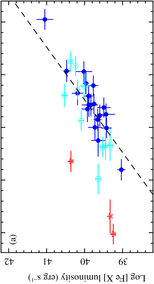
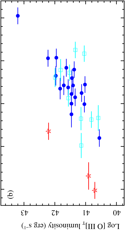
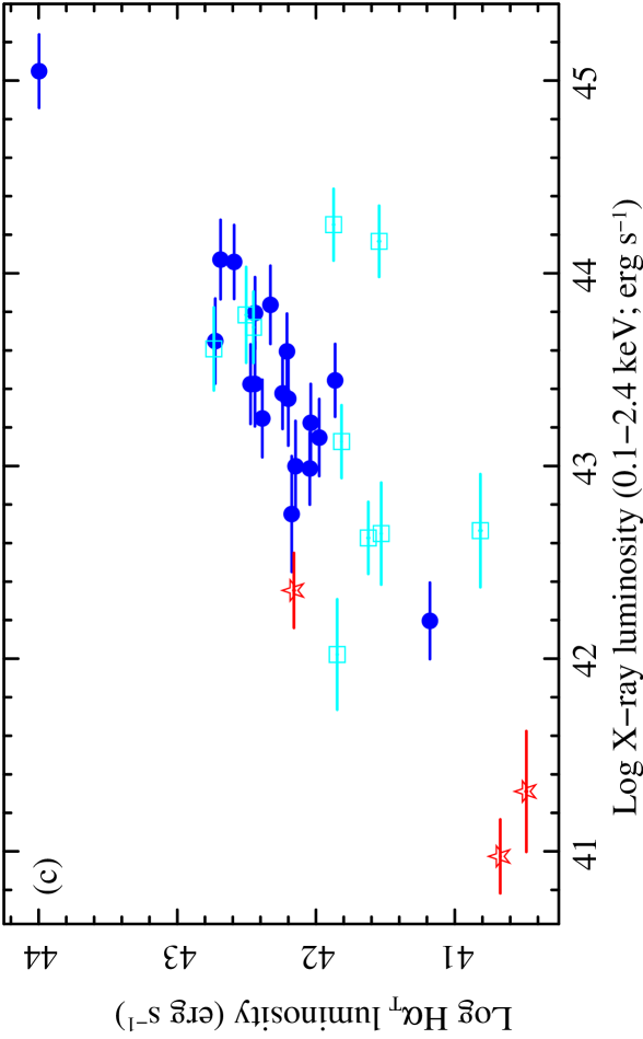
Figure 12: Luminosities of $[\mathrm{Fe}\,\mbox{{x}}]$, $[\mathrm{O}\,\mbox{{iii}}]_{T}$, and $\mathrm{H}\alpha_{T}$ (panels a–c, respectively) vs. $L_{x}$ in the observed 0.1–2.4 keV band. Point styles and the dashed line are as in Fig. 11 (the error bars for $[\mathrm{O}\,\mbox{{iii}}]_{T}$ and $\mathrm{H}\alpha_{T}$ are smaller than the points). Panels a and b demonstrate that the line and X-ray powers of type 1 Seyferts are correlated, but the Sy2s are offset by more than an order of magnitude in $L_{x}$; in panel c the Sy2s, whose $\mathrm{H}\alpha_{T}$ lines lack a broad component, lie closer to the type 1 objects. An inspection of the type 1 Seyferts shows that the relationships of $[\mathrm{O}\,\mbox{{iii}}]_{T}$ and $\mathrm{H}\alpha_{T}$ with $L_{x}$ exhibit more scatter than $[\mathrm{Fe}\,\mbox{{x}}]$, although in the case of $\mathrm{H}\alpha_{T}$ the additional scatter is primarily due to a few outliers (see §5.4). We note that whilst these plots are affected by Malmquist bias, they still offer a fair representation of the relative amounts of scatter amongst the different correlations.

5 Discussion

5.1 Line profiles, IPs and FHIL kinematics

The $[\mathrm{Fe}\,\mbox{{x}}]$ and $[\mathrm{Fe}\,\mbox{{xi}}]$ lines are expected to be well correlated because they have similar IPs (234 and 262 eV, respectively) and $N_{cr}$ ($10^{9.7}$ and $10^{10.4}\ \mathrm{cm}^{-3}$). Indeed, we find that their fluxes are essentially indistinguishable (§4.2), and they have mutually-consistent profiles in more than half of the sample members with $[\mathrm{Fe}\,\mbox{{xi}}]$ detections. However, in the remaining sources the $[\mathrm{Fe}\,\mbox{{xi}}]$ lines tend to be both broader and bluer than $[\mathrm{Fe}\,\mbox{{x}}]$. This suggests that the distribution of $[\mathrm{Fe}\,\mbox{{xi}}]$-emitting clouds sometimes extends closer to the BLR, probing a region where the outflow velocities are higher. Similar evidence has been shown for selected objects in smaller samples (e.g., Erkens et al., 1997; Mullaney & Ward, 2008).

The velocity shifts of $[\mathrm{Fe}\,\mbox{{vii}}]_{1G}$ are similar to, and well correlated with, those of $[\mathrm{Fe}\,\mbox{{x}}]$, suggesting that the clouds responsible for the core of the $[\mathrm{Fe}\,\mbox{{vii}}]$ profile are part of the same flow as the $[\mathrm{Fe}\,\mbox{{x}}]$-emitting clouds. However, there is only a weak correlation between the widths of these components. It is therefore unlikely that the $[\mathrm{Fe}\,\mbox{{vii}}]_{1G}$ and $[\mathrm{Fe}\,\mbox{{x}}]$ lines are dominated by the same clouds. An alternative hypothesis is that they are from spatially distinct regions of an outflow that is “coasting”, neither accelerated nor decelerated significantly between the $[\mathrm{Fe}\,\mbox{{x}}]$- and $[\mathrm{Fe}\,\mbox{{vii}}]$-emitting portions of the flow. In such a scenario the $[\mathrm{Fe}\,\mbox{{vii}}]$ clouds are expected to be the downstream component due to the lower ionisation parameter required and may be more readily resolved spatially. This is consistent with our recent photoionisation models of FHIL emission in the NLS1 Ark 564, from which we infer that clouds in a radiatively-driven outflow are accelerated before the FHIL becomes strong. The terminal velocity is approached and Fe is released within the clouds as dust grains become sublimated (Mullaney et al., 2009). We note further that the wings of $[\mathrm{O}\,\mbox{{iii}}]$ are outflowing and may be related to the $[\mathrm{Fe}\,\mbox{{x}}]$- and/or $[\mathrm{Fe}\,\mbox{{vii}}]_{1G}$-emitting portion of the outflow, as the average $[\mathrm{O}\,\mbox{{iii}}]_{W}$ velocity shifts amongst the NLS1s, Sy1.0s and Sy1.5s are consistent with those of these FHILs (cf. §4.3). On the other hand, the velocity shifts of $[\mathrm{O}\,\mbox{{iii}}]_{C}$ and the lower-ionisation narrow lines are consistent with that of $[\mathrm{S}\,\mbox{{ii}}]$ and are not part of this flow.

5.2 Line correlations with X-rays

In §4.4 we show that the $[\mathrm{Fe}\,\mbox{{x}}]$ lines of type 1 Seyferts scale rather well with X-ray flux, in agreement with previous studies (Porquet et al., 1999). However, we note a systematic difference between the NLS1 and BLS1s. This is made clear by the offset between the linear correlations fitted to these two populations in Fig. 11. One contributor to this is likely to be our simplistic assumption of a uniform spectral model to convert Rosat count rates to fluxes. NLS1s have long been known to have, on average, stronger soft excess and steeper soft X-ray spectra (e.g., Boller, 2000). If we adopt a steeper spectral index for these objects ($\Gamma=3.0$ instead of 1.5) and plot $[\mathrm{Fe}\,\mbox{{x}}]$ flux against just the estimated 233–300 eV flux (which dominates the photoionisation of $[\mathrm{Fe}\,\mbox{{x}}]$ and $[\mathrm{Fe}\,\mbox{{xi}}]$), the offset between the NLS1 and BLS1 distributions disappears (Fig. 13). Thus, it appears that a single correlation between the $[\mathrm{Fe}\,\mbox{{x}}]$ and soft X-ray fluxes applies to both NLS1s and BLS1s. It follows that observations of coronal lines may be used to constrain the SED at soft X-ray energies when observations in this band are either not available or of low sensitivity. The average ratio we obtain for $\log([\mathrm{Fe}\,\mbox{{x}}]/F_{\mathrm{233-300eV}})$ is $-2.03\pm 0.07$ with an RMS of 0.36. Additionally, we note that the NLS1 and BLS1 distributions are not as clearly separated in the $[\mathrm{O}\,\mbox{{iii}}]_{T}$-$L_{x}$ or $\mathrm{H}\alpha_{T}$-$L_{x}$ planes (Fig. 12b–c). Inaccuracies in the assumed spectral indices of NLS1s should have a smaller effect upon these correlations because, unlike $[\mathrm{Fe}\,\mbox{{x}}]$, the $[\mathrm{O}\,\mbox{{iii}}]_{T}$ and $\mathrm{H}\alpha_{T}$ line emission is not particularly responsive to any specific portion of the X-ray band. Consequently, they should scale more directly with the bolometric power, hence the overall Rosat luminosity, the estimate of which is less sensitive to the model used to interpret PSPC count rates.

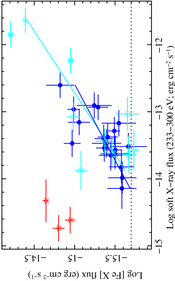
Figure 13: $[\mathrm{Fe}\,\mbox{{x}}]$ vs. soft X-ray flux. The soft band is the portion of the X-ray spectrum most directly responsible for photoionising $[\mathrm{Fe}\,\mbox{{x}}]$. Here we estimate the 233–300 keV flux with the further assumption that NLS1s have a softer X-ray spectrum ($\Gamma=3.0$). As a result the difference between the $[\mathrm{Fe}\,\mbox{{x}}]$/X-ray ratios of NLS1s and BLS1s essentially disappears (compare to Fig. 11). This is demonstrated by the linear correlations fitted to these two populations (cyan and blue solid lines, respectively). The horizontal dashed line is once again the approximate $[\mathrm{Fe}\,\mbox{{x}}]$ flux limit and the point styles are the same as in Fig. 11.

The amount of scatter in the emission line vs. X-ray correlations allows us to put constraints on the size of the line emitting regions and the variability history of the AGN. In principle the lines should scale with the bolometric power of the central engine, hence they should correlate with the X-ray flux. However, any variability of the photoionising continuum strength will weaken the observed correlation because the Rosat data provide a snapshot of the AGN power at a moment in time, whereas the line emitting regions are extended and therefore the observed lines are a response to the AGN power averaged over the light-crossing time of these regions. The more variable the bolometric power is, on time-scales much shorter than either the light-crossing time of the line-emitting regions or the time lag between the X-ray and optical spectroscopic observations, the more likely it becomes that the instantaneous X-ray power observed would not be representative of the time-averaged power affecting the measured lines. The relatively modest scatter found amongst the type 1 Seyferts in Fig. 13 (0.38 dex) indicates that the instantaneous X-ray power measured by Rosat was within a factor of a few of the time-averaged power to which the FHILs were responding when observed by SDSS 10–15 years later. Thus, none of our sources appear to have been caught in a short time-scale X-ray fluctuation at the time of the Rosat observation, or a several-year drift in power since that time, by more than a factor of a few. A contribution to the scatter in the emission line vs. X-ray plots is the made by the model dependence inherent in converting Rosat count rates to fluxes, which in the most extreme cases could introduce $F_{x}$ errors up to a factor of two. We note that the scatter exhibited by the NLS1 is much larger than that of the BLS1 distribution in Fig. 13 (0.48 vs. 0.27 dex). This could be due to either variability or greater inaccuracies in the models used to interpret the count rates, as NLS1s are known both to be more variable and to exhibit a wider range of spectral indices in the soft X-ray band.

The fact that the correlation between $[\mathrm{Fe}\,\mbox{{vii}}]_{T}$ and X-rays is weaker with much more scatter than that between $[\mathrm{Fe}\,\mbox{{x}}]$ and X-rays suggests that the $[\mathrm{Fe}\,\mbox{{vii}}]$-emitting clouds are much more extended than those of $[\mathrm{Fe}\,\mbox{{x}}]$. The longer light-crossing time of a more extended region gives the central engine more time to drift away from the time-averaged power to which the $[\mathrm{Fe}\,\mbox{{vii}}]$ line is responding. Other sources of noise in this correlation are less likely because (1) there is not likely to be much photoionised $[\mathrm{Fe}\,\mbox{{vii}}]$ emission that is unrelated to the AGN because the stellar continuum power above the IP energy of 99 eV is negligible, and (2) the correlation between the velocities of $[\mathrm{Fe}\,\mbox{{vii}}]_{1G}$ and $[\mathrm{Fe}\,\mbox{{x}}]$ (Fig. 10) connect the $[\mathrm{Fe}\,\mbox{{vii}}]$-emitting clouds to the $[\mathrm{Fe}\,\mbox{{x}}]$-bearing outflow, demonstrating both that the $[\mathrm{Fe}\,\mbox{{vii}}]$-emitting medium likely originates in the AGN and showing no sign of the deceleration that would take place if this flow were shocked. Furthermore, the similarity of the $[\mathrm{Fe}\,\mbox{{vii}}]$–X-ray correlation to those between various narrow lines and X-rays, and the strong correlations between $[\mathrm{Fe}\,\mbox{{vii}}]$ and the NLR lines (notably $[\mathrm{O}\,\mbox{{i}}]$ and $[\mathrm{O}\,\mbox{{iii}}]$) suggests that the $[\mathrm{Fe}\,\mbox{{vii}}]$-emitting region merges with that of the traditional NLR. This is corroborated by previous studies which have shown that unlike coronal lines with higher IPs and $N_{cr}$, the measured profiles of $[\mathrm{Fe}\,\mbox{{vii}}]$ are often consistent with those of the lower-ionisation forbidden lines (Veilleux, 1991).

5.3 Structure of the FHIL-emitting region

What is the geometry of the FHIL-emitting region of Seyfert galaxies? MT98 found that amongst a sample of 35 Seyferts mostly collected from the literature, type 2 Seyferts have significantly lower $[\mathrm{Fe}\,\mbox{{vii}}]$/$[\mathrm{O}\,\mbox{{iii}}]$ flux ratios than type 1s, suggesting that at least part of the $[\mathrm{Fe}\,\mbox{{vii}}]$-emitting region is obstructed along our line of sight in Seyfert 2 galaxies. From this they infer that some of the $[\mathrm{Fe}\,\mbox{{vii}}]$ emission arises from regions hidden from our view by the same structure that obscures the BLR in Sy2s, the circumnuclear torus. NTM00 reaffirm this result using an expanded sample (Fig. 7) and report a similar, albeit weaker, disparity in the distributions of $[\mathrm{Fe}\,\mbox{{x}}]/[\mathrm{O}\,\mbox{{iii}}]$ ratios, therefore concluding that the $[\mathrm{Fe}\,\mbox{{x}}]$-emitting clouds are less obscured than those responsible for the $[\mathrm{Fe}\,\mbox{{vii}}]$ emission. These authors therefore argue that a significant fraction of the $[\mathrm{Fe}\,\mbox{{vii}}]$ flux arises from material at the inner surface of the torus, whereas a larger fraction of the $[\mathrm{Fe}\,\mbox{{x}}]$ emission arises from a larger-scale region. On the other hand, several other authors have interpreted the correlation between critical densities, ionisation potentials, and the width of the line profiles as evidence for a stratified line-emitting region in which the clouds responsible for the FHILs extend from the outer reaches of the BLR through the NLR, with the highest-ionisation lines arising closest to the BLR (De Robertis & Osterbrock, 1984, 1986; Appenzeller & Öestreicher, 1988; Rodríguez-Ardila et al., 2002).

As described in §4.2, we do not find any significant difference between the $[\mathrm{Fe}\,\mbox{{vii}}]$/$[\mathrm{O}\,\mbox{{iii}}]$ ratios of type 1 and type 2 Seyferts, in contradiction with MT98 and NTM00. We do find that the $[\mathrm{Fe}\,\mbox{{x}}]$/$[\mathrm{Fe}\,\mbox{{vii}}]_{T}$ ratios differ between the spectral types, but these differences are the opposite of what would be expected from the NTM00 results. The mean averages of the log ratios we obtain are $0.03\pm 0.13$, $-0.24\pm 0.04$, and $-0.44\pm 0.06$ for NLS1s, BLS1s and Sy2s, respectively. There is considerable overlap in the distributions (see the histogram at the top of Fig. 14), but the probability that the NLS1s and Sy2s are drawn from populations with the same ratio distribution is less than 0.001 per cent according to a KS test. The interpretation of these differences could be either an excess of $[\mathrm{Fe}\,\mbox{{vii}}]$ or a deficiency of $[\mathrm{Fe}\,\mbox{{x}}]$ amongst Sy2s and the opposite situation amongst NLS1, as will be discussed below. Note, however, that the average ratio of the NLS1s is increased significantly by three outliers with $\log([\mathrm{Fe}\,\mbox{{x}}]/[\mathrm{Fe}\,\mbox{{vii}}])>0.6$. If these extreme sources are omitted, the mean ratio amongst the remaining 9 NLS1s ($-0.19\pm 0.05$) is consistent with that of the BLS1s. Thus, the NLS1s may represent a heterogeneous population that includes some objects with rather extreme properties and some that more closely resemble broad-lined Sy1s.

Differences between the best-fitting $[\mathrm{Fe}\,\mbox{{x}}]$ model parameters of type 1 and type 2 Seyferts provide evidence that the low $[\mathrm{Fe}\,\mbox{{x}}]$/$[\mathrm{Fe}\,\mbox{{vii}}]$ ratios amongst Sy2s is due to partially-obscured $[\mathrm{Fe}\,\mbox{{x}}]$ emission. In Seyfert 2s these lines tend to be narrower and have lower fluxes relative to $[\mathrm{Fe}\,\mbox{{vii}}]$ (Fig. 14). This is consistent with a scenario in which the part of the $[\mathrm{Fe}\,\mbox{{x}}]$-emitting region that contributes the broadest line flux generally cannot be observed in Seyfert 2 galaxies, and in which the $[\mathrm{Fe}\,\mbox{{vii}}]$-emitting region is less affected by obscuration.

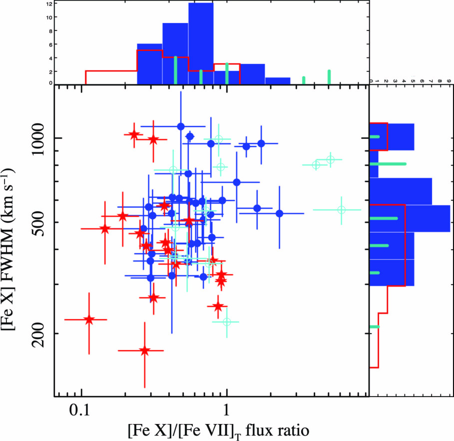
Figure 14: $[\mathrm{Fe}\,\mbox{{x}}]$ line width vs. $[\mathrm{Fe}\,\mbox{{x}}]$/$[\mathrm{Fe}\,\mbox{{vii}}]_{T}$ flux ratio. Point styles as in Fig. 8; histogram styles as in Fig. 4 (top). The Sy2s on average have less $[\mathrm{Fe}\,\mbox{{x}}]$ power per unit of $[\mathrm{Fe}\,\mbox{{vii}}]$ power than either the BLS1s or the NLS1s, although the histogram at the top demonstrates that the distributions are broad with substantial overlap. The histogram at right shows that the $[\mathrm{Fe}\,\mbox{{x}}]$ lines tend to be narrower in Seyfert 2s. Taken together, these suggest that a part of the $[\mathrm{Fe}\,\mbox{{x}}]$-emitting region, the part that contributes the broadest line flux, is often hidden from us in Sy2s.

5.4 NLS1s with extreme [Fe X]/[O III] ratios

In the preceding sections it was noted that a few NLS1s have extreme line ratios that cause them to stand out from both the other NLS1s and the other sample members in general (see Figs. 8 and 12 and the discussion of $[\mathrm{Fe}\,\mbox{{x}}]$/$[\mathrm{Fe}\,\mbox{{vii}}]$ flux ratios in §5.3). Two NLS1s in particular, sources 25 and 50, are consistently the most extreme outliers whenever there are outliers to a correlation. For instance, these are the only two sample members with $\log([\mathrm{Fe}\,\mbox{{x}}]/[\mathrm{O}\,\mbox{{iii}}]_{T})>-1.0$, whereas the mean for the rest of the sample is $-1.66\pm 0.04$ with an $\mathrm{RMS}=0.28$. In addition to their extreme line ratios, these sources have two of the narrowest $\mathrm{H}\alpha_{B}$ lines in our sample (FWHM values of $745\pm 2$ and $780\pm 2\ \mathrm{km\,s^{-1}}$ respectively). What is it about these NLS1s that sets them apart from the rest of the sample?

Not every pair of correlated parameters has significant outliers. For instance, there are no outliers in the $[\mathrm{Fe}\,\mbox{{x}}]$–$[\mathrm{Fe}\,\mbox{{xi}}]$ plane (Fig. 6), nor if we plot $[\mathrm{O}\,\mbox{{i}}]$ vs. $[\mathrm{O}\,\mbox{{iii}}]_{T}$ (Fig. 15a). As discussed earlier, $[\mathrm{Fe}\,\mbox{{x}}]$ and $[\mathrm{Fe}\,\mbox{{xi}}]$ emission lines both respond to the continuum in the soft X-ray band. We therefore expect these three fluxes to be closely correlated. This is found to be the case for the present sample, without exception. Likewise, we do not find any obvious outliers when we compare fluxes of pairs of NLR features (such as $[\mathrm{O}\,\mbox{{iii}}]$, $[\mathrm{O}\,\mbox{{i}}]$, $[\mathrm{N}\,\mbox{{ii}}]$, or $\mathrm{H}\alpha_{N}$). It is only when we compare fluxes between these two groups that the outliers tend to stand out, with high ratios of $[\mathrm{Fe}\,\mbox{{x}}]$ (or $[\mathrm{Fe}\,\mbox{{xi}}]$ or X-rays) over NLR fluxes. These groups may be thought of as compact and extended emission regions, or as high- and low-energy processes.

It appears that for the two consistent outliers the relationship between the smaller-scale/higher-energy processes and the larger-scale/lower-energy features differs from that of most other Seyferts. Two possible causes for this disconnect are variability and differences in the broad-band spectral shapes. If the average power of the AGN has changed relatively recently (10–100 years or so), then the compact FHIL-emitting region will have had time to respond but the more extended NLR will not. Alternatively, these outliers may be affected by a broadband spectral feature that is not present (or as prominent) in other sample members. Erkens et al. (1997) have suggested that AGNs with strong excesses in the soft X-ray band tend to produce strong FHILs, based upon the correlation they demonstrated between the $[\mathrm{Fe}\,\mbox{{x}}]$ equivalent widths and the photon index of Rosat data. An extreme soft excess would provide a disproportionate supply of $\sim 250\ \mathrm{eV}$ photons, thereby producing extra FHIL emission through photoionisation; lines that respond to other parts of the continuum will not be affected so their relative strength will be lower. It is worth noting that one of these outliers is KUG 1031+398, which has one of the strongest soft excesses known (Puchnarewicz et al., 2001; Middleton, Done & Gierliński, 2007). We note further that the two outliers have the lowest HR1 values of all the RASS-detected members of the sample (HR1 = hardness ratio for the low energy end of the Rosat band), suggesting that source 50 may also have a strong soft excess.

The observation that both of our consistent outliers may have strong excesses in the soft X-ray band is suggestive that the mechanism that causes them to stand out relates to the SED shape, but with just two objects this does not rule out the possibility that these sources stand out due to variability. To break the degeneracy between an origin relating to the scale size and one relating to the SED, we consider $\mathrm{H}\alpha_{B}$. The BLR is more compact than the FHIL-emitting region but $\mathrm{H}\alpha$ emission is not specifically sensitive to the soft X-ray continuum. In Fig. 12c, the two data points farthest from the $\mathrm{H}\alpha_{T}$–$L_{x}$ correlation are sources 25 and 50, whereas Fig. 17b shows that there are no egregious outliers in the $[\mathrm{O}\,\mbox{{iii}}]_{T}$–$\mathrm{H}\alpha_{T}$ plane. Thus, the $\mathrm{H}\alpha_{B}$ emission in these objects tracks with the larger-scale/lower-energy features and not the smaller-scale/higher-energy features, indicating that sources 25 and 50 behave differently from most of the sample due to a difference in their SEDs, not variability.

If sources 25 and 50 do have strong soft excesses, and if this feature of their SED affects the emission lines, then we can use the emission lines to constrain portions of the soft excess that are difficult to observe directly. Specifically, we can use the strength of $[\mathrm{Fe}\,\mbox{{vii}}]$ relative to other features to constrain the photoionising continuum around 100 eV. We find that these sources are outliers in the $[\mathrm{Fe}\,\mbox{{vii}}]$–$[\mathrm{Fe}\,\mbox{{x}}]$ flux plane (Fig. 8) but not in the $[\mathrm{Fe}\,\mbox{{vii}}]$–$[\mathrm{O}\,\mbox{{iii}}]$ plane (Fig. 16c). Thus it appears that the $[\mathrm{Fe}\,\mbox{{vii}}]$ lines do not respond strongly to the soft excess: either this spectral component does not extend down to 100 eV or the bulk of the $[\mathrm{Fe}\,\mbox{{vii}}]$-emitting region is shielded from this photoionising continuum by intrinsic absorption.

6 Summary and conclusions

We have used $[\mathrm{Fe}\,\mbox{{x}}]$ line emission to select a sample of galaxies from the SDSS with strong forbidden high-ionisation line (FHIL) emission. The resulting 63 Seyfert galaxies comprise the first ever FHIL-selected sample of AGN. Moreover, it is the most homogeneous and one of the largest samples of FHIL-emitting galaxies to date. In each of these spectra we have measured the strengths and profiles of several emission lines (including $[\mathrm{Fe}\,\mbox{{x}}]$, $[\mathrm{Fe}\,\mbox{{xi}}]$, $[\mathrm{Fe}\,\mbox{{vii}}]$, $[\mathrm{O}\,\mbox{{iii}}]$ and $\mathrm{H}\alpha$). We have also included soft X-ray data for all objects with available Rosat measurements. From our analysis of these data we conclude:

• That the $[\mathrm{Fe}\,\mbox{{x}}]$ and $[\mathrm{Fe}\,\mbox{{xi}}]$ lines are well correlated with both each other and the soft X-ray continuum flux, with a mean $[\mathrm{Fe}\,\mbox{{x}}]$/$F_{\mathrm{233-300eV}}$ ratio of $9.4\times 10^{-3}$. Their correlation with the X-ray strength supports a photoionisation origin of these line species, rather than collisional. The correlation with X-rays applies to all type 1 Seyferts and may be used to estimate soft X-ray fluxes based upon observed FHIL strengths.

• There are significant differences in the $[\mathrm{Fe}\,\mbox{{x}}]$/$[\mathrm{Fe}\,\mbox{{vii}}]$ ratios between narrow-lined Seyfert 1s (NLS1s), broad-lined Seyfert 1s (BLS1s, including both 1.0 and intermediate type 1.5 Seyferts), and Seyfert 2s (Sy2s), either because of selective absorption of the $[\mathrm{Fe}\,\mbox{{x}}]$ or because of a different ionising continuum. In the Sy2s the ratios of $[\mathrm{Fe}\,\mbox{{x}}]$/$[\mathrm{Fe}\,\mbox{{vii}}]$ tend to be lower and the FWHM of the $[\mathrm{Fe}\,\mbox{{x}}]$ line profiles are narrower. These facts suggest that some fraction of the $[\mathrm{Fe}\,\mbox{{x}}]$ flux (i.e., the broad component) may be hidden in Sy2s, possibly because it is emitted in a region of size comparable to the dusty molecular torus. A subset of NLS1s have high $[\mathrm{Fe}\,\mbox{{x}}]$/$[\mathrm{Fe}\,\mbox{{vii}}]$ and $[\mathrm{Fe}\,\mbox{{x}}]$/$[\mathrm{O}\,\mbox{{iii}}]$ ratios, which is consistent with an over production of $[\mathrm{Fe}\,\mbox{{x}}]$ in response to an excess of ionising photons in the soft X-ray band.

• Using the low ionisation lines of $[\mathrm{S}\,\mbox{{ii}}]$ as a proxy for the systemic velocity of the host galaxy, we find that $[\mathrm{Fe}\,\mbox{{xi}}]$, $[\mathrm{Fe}\,\mbox{{x}}]$ and $[\mathrm{Fe}\,\mbox{{vii}}]$ are generally blueshifted with velocities of order 100 $\mathrm{km\,s^{-1}}$. The most blueshifted lines tend to have the broadest profiles. In particular, about 1/3 of $[\mathrm{Fe}\,\mbox{{xi}}]$ lines are both broader and bluer than the other FHILs. The $[\mathrm{O}\,\mbox{{iii}}]$ lines are found to have blue wings with widths and velocities comparable to those of the FHILs and narrow cores at the systemic velocity.

• In our correlations there are a few sources that consistently are far from the general trends. These outliers are type 1 Seyferts that have the narrowest $\mathrm{H}\alpha_{B}$ lines amongst our NLS1s and the softest X-ray spectra amongst our entire sample. Their deviations from the overall trends may be manifestations of important intrinsic differences between examples of very narrow line BLRs and the majority of Seyfert 1s.

• The good correlation between $F_{x}$ and $[\mathrm{Fe}\,\mbox{{x}}]$ emission observed 10–15 years later means that the measured X-ray flux (an instantaneous snapshot) is relatively representative of average X-ray power to which the FHIL-emitting region responds. It follows that variability over time-scales ranging from that of the Rosat exposure times to the lag time of the SDSS observations (several minutes to several years) is usually no more than a factor of a few.

These findings are consistent with a stratified wind model, in which outflowing photoionised clouds produce $[\mathrm{Fe}\,\mbox{{xi}}]$, $[\mathrm{Fe}\,\mbox{{x}}]$, $[\mathrm{Fe}\,\mbox{{vii}}]$ and possibly the wings of $[\mathrm{O}\,\mbox{{iii}}]$. The $[\mathrm{Fe}\,\mbox{{xi}}]$- and $[\mathrm{Fe}\,\mbox{{x}}]$-emitting clouds lie closest to the BLR at a scale comparable to the obscuring torus, which sometimes cover a significant fraction of these clouds in Seyfert 2s. $[\mathrm{Fe}\,\mbox{{vii}}]$, in comparison to $[\mathrm{Fe}\,\mbox{{x}}]$ and $[\mathrm{Fe}\,\mbox{{xi}}]$, is found to correlate less well with $F_{x}$ and better with $[\mathrm{O}\,\mbox{{iii}}]$; it is also apparently not affected when the $[\mathrm{Fe}\,\mbox{{x}}]$ emitting region is partially covered. These facts suggest that the $[\mathrm{Fe}\,\mbox{{vii}}]$-emitting region is more extended and may approach the scale of the NLR. However, the correlation between $[\mathrm{Fe}\,\mbox{{vii}}]$ and $[\mathrm{Fe}\,\mbox{{x}}]$ fluxes and in particular the similarity of their velocity shifts implies that the clouds emitting these features are related to each other and may be different parts of the same outflow. The narrow cores of $[\mathrm{O}\,\mbox{{iii}}]$ and the other low ionisation species such as $[\mathrm{O}\,\mbox{{i}}]$ do not have a velocity shift relative to $[\mathrm{S}\,\mbox{{ii}}]$; the clouds emitting these lines are either a decelerated portion of the outflow or are unrelated to it.

Based upon the strong correlation between $[\mathrm{Fe}\,\mbox{{x}}]$ and soft X-ray flux (§5.2) and our discussion of the sources that appear to be exceptions to the overall correlations found in the sample (§5.4), we infer that strong $[\mathrm{Fe}\,\mbox{{x}}]$ emission (relative to other optical lines such as $[\mathrm{O}\,\mbox{{iii}}]$ and $[\mathrm{Fe}\,\mbox{{vii}}]$) is an optical-wavelength indicator of strong soft excesses in the X-ray band. Furthermore, the fact that these same objects do not have high $[\mathrm{Fe}\,\mbox{{vii}}]$/$[\mathrm{O}\,\mbox{{iii}}]$ ratios suggests that these soft excesses either do not continue through $\sim 100$ eV into the difficult–to–observe EUV band or the $[\mathrm{Fe}\,\mbox{{vii}}]$-emitting clouds are shielded from the soft excess by intrinsic absorption. The connection between FHIL emission and the intrinsic continuum in the few hundred eV range needs to be tested with better X-ray data. A more detailed analysis of the available X-ray data would be useful, but the number of $[\mathrm{Fe}\,\mbox{{x}}]$-selected sources with available X-ray spectra is severely limited. New observations would be necessary to better calibrate the FHIL–X-ray correlations.

Finally, we note that our $[\mathrm{Fe}\,\mbox{{x}}]$ selection yielded only one object that is not obviously an AGN (source 45 here; Ward et al. in preparation). This confirms that it is exceptionally rare for non-active galaxies to produce strong FHIL emission. However, we cannot quantify just how rare this is (or what fraction of AGN are strong FHIL emitters, or whether one Seyfert class is more likely than another to have strong FHILs) because the present study does not include a control group. To remedy this, we are conducting a broader search for FHIL emission amongst a much larger sample of SDSS emission line galaxies. This next step will reduce selection effects in the present sample and will better enable us to put $[\mathrm{Fe}\,\mbox{{x}}]$-selected sources into context.

Appendix A Online supplementary material

Online we provide Tables 7–16 in which we present the parameters of our best-fitting models to the emission lines in the SDSS spectra. In Table 18 we provide the compiled Rosat count data used in this study: count rates from the Rosat All-Sky Survey (RASS; Voges et al., 1999, 2000) and the White, Giommi & Angelini (2000) Catalogue of sources found in pointed Rosat observations, RASS hardness ratios, and flux estimates based upon these count rates.

Also provided online are a set of figures showing various line luminosities plotted against the luminosities of $[\mathrm{O}\,\mbox{{i}}]$ (Fig. 15), $[\mathrm{O}\,\mbox{{iii}}]_{T}$ (16), $\mathrm{H}\alpha_{T}$ (17), $[\mathrm{Fe}\,\mbox{{x}}]$ (18), 0.1–2.4 keV X-rays (19).

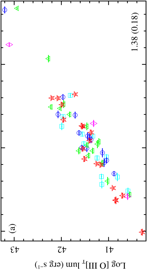
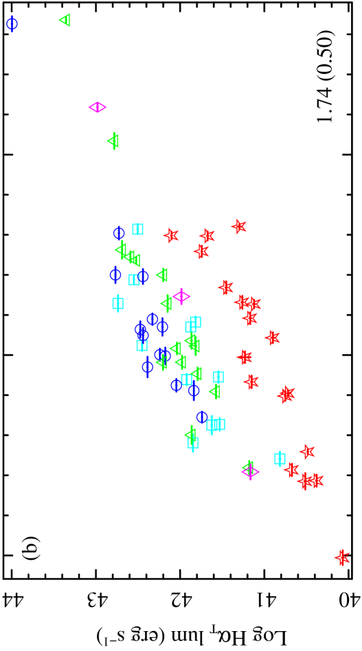
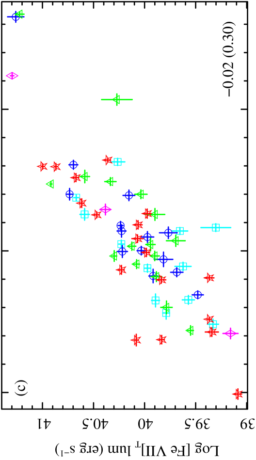
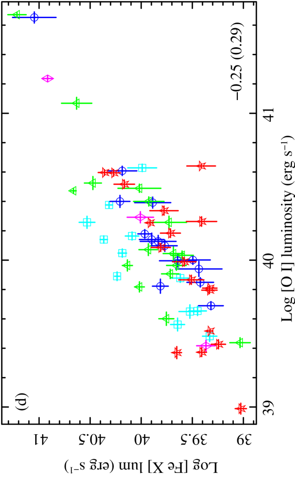
Figure 15: Luminosities of (a) $[\mathrm{O}\,\mbox{{iii}}]_{T}$, (b) $\mathrm{H}\alpha_{T}$, (c) $[\mathrm{Fe}\,\mbox{{vii}}]_{T}$, and (d) $[\mathrm{Fe}\,\mbox{{x}}]$ vs. $[\mathrm{O}\,\mbox{{i}}]$. Spectral classifications are indicated by point colors and styles as follows: NLS1 = cyan squares, Sy1.0 = blue circles, Sy1.5 = green triangles, Sy1.9 = magenta diamonds, and Sy2 = red stars. The numbers in the lower-right corners are the mean of the log ( line / $[\mathrm{O}\,\mbox{{i}}]$ ) values, with the RMS about this average ratio given in parenthesis.

Table 7: Best-fitting $[\mathrm{Fe}\,\mbox{{x}}]$ models.

ID	FWHM		$v_{\mathrm{sh}}$		Flux		EqW		$\Delta\chi^{2}$
	($\mathrm{km\,s^{-1}}$)		($\mathrm{km\,s^{-1}}$)		($\times 10^{-16}$)		(Å)
1	560$\,\pm\,$	90	-50$\,\pm\,$	40	2.4$\,\pm\,$	0.5	1.1$\,\pm\,$	0.2	81.5
2	770$\,\pm\,$	140	-30$\,\pm\,$	60	4.2$\,\pm\,$	1.0	1.3$\,\pm\,$	0.3	59.8
3	360$\,\pm\,$	40	-248.$\,\pm\,$	19.	16.$\,\pm\,$	3.	0.73$\,\pm\,$	0.12	135.0
4	590$\,\pm\,$	170	20$\,\pm\,$	70	2.6$\,\pm\,$	1.0	0.7$\,\pm\,$	0.3	25.3
5	990$\,\pm\,$	170	260$\,\pm\,$	70	4.5$\,\pm\,$	1.0	1.9$\,\pm\,$	0.4	68.2
6	510$\,\pm\,$	80	-10$\,\pm\,$	40	1.9$\,\pm\,$	0.4	2.5$\,\pm\,$	0.5	77.2
7	570$\,\pm\,$	40	-160.$\,\pm\,$	19.	19.$\,\pm\,$	2.	1.86$\,\pm\,$	0.20	295.6
8	350$\,\pm\,$	60	-160$\,\pm\,$	30	2.1$\,\pm\,$	0.5	1.3$\,\pm\,$	0.3	67.5
9	530$\,\pm\,$	120	-130$\,\pm\,$	50	3.6$\,\pm\,$	1.1	0.8$\,\pm\,$	0.2	34.8
10	320$\,\pm\,$	60	-100$\,\pm\,$	20	4.4$\,\pm\,$	1.1	0.70$\,\pm\,$	0.17	55.6
11	360$\,\pm\,$	60	-100$\,\pm\,$	30	1.8$\,\pm\,$	0.4	0.88$\,\pm\,$	0.19	75.0
12	590$\,\pm\,$	190	-330$\,\pm\,$	90	6.$\,\pm\,$	3.	0.5$\,\pm\,$	0.2	15.5
13	530$\,\pm\,$	110	60$\,\pm\,$	50	4.6$\,\pm\,$	1.3	0.72$\,\pm\,$	0.20	40.2
14	360$\,\pm\,$	40	-19.$\,\pm\,$	19.	3.2$\,\pm\,$	0.5	1.02$\,\pm\,$	0.16	153.4
15	400$\,\pm\,$	80	-70$\,\pm\,$	30	3.1$\,\pm\,$	0.8	1.0$\,\pm\,$	0.3	22.0
16	540$\,\pm\,$	130	-40$\,\pm\,$	60	1.8$\,\pm\,$	0.6	1.7$\,\pm\,$	0.5	32.6
17	460$\,\pm\,$	50	0$\,\pm\,$	20	3.7$\,\pm\,$	0.6	2.2$\,\pm\,$	0.3	150.8
18	320$\,\pm\,$	30	-60.$\,\pm\,$	12.	5.0$\,\pm\,$	0.6	2.6$\,\pm\,$	0.3	303.8
19	380$\,\pm\,$	60	-90$\,\pm\,$	20	2.8$\,\pm\,$	0.5	1.7$\,\pm\,$	0.3	93.6
20	790$\,\pm\,$	60	10$\,\pm\,$	20	62.$\,\pm\,$	6.	2.1$\,\pm\,$	0.2	373.1
21	390$\,\pm\,$	70	-50$\,\pm\,$	30	11.$\,\pm\,$	2.	0.76$\,\pm\,$	0.17	68.4
22	540$\,\pm\,$	40	-54.$\,\pm\,$	19.	8.7$\,\pm\,$	1.0	4.1$\,\pm\,$	0.5	262.5
23	600$\,\pm\,$	70	-250$\,\pm\,$	30	10.3$\,\pm\,$	1.7	1.4$\,\pm\,$	0.2	119.2
24	220$\,\pm\,$	30	-87.$\,\pm\,$	11.	1.9$\,\pm\,$	0.3	1.5$\,\pm\,$	0.2	134.7
25	800$\,\pm\,$	30	-352.$\,\pm\,$	14.	41.$\,\pm\,$	2.	5.5$\,\pm\,$	0.3	993.4
26	1100$\,\pm\,$	400	-380$\,\pm\,$	160	2.8$\,\pm\,$	1.3	1.0$\,\pm\,$	0.4	17.4
27	550$\,\pm\,$	60	-30$\,\pm\,$	30	3.5$\,\pm\,$	0.5	3.6$\,\pm\,$	0.5	150.8
28	1400$\,\pm\,$	300	-40$\,\pm\,$	90	8.$\,\pm\,$	2.	3.3$\,\pm\,$	0.9	104.3
29	530$\,\pm\,$	70	-260$\,\pm\,$	30	3.2$\,\pm\,$	0.6	1.9$\,\pm\,$	0.4	93.9
30	320$\,\pm\,$	120	130$\,\pm\,$	50	2.2$\,\pm\,$	1.0	0.41$\,\pm\,$	0.20	16.3
31	420$\,\pm\,$	30	-30.$\,\pm\,$	15.	10.7$\,\pm\,$	1.2	2.1$\,\pm\,$	0.2	290.1
32	610$\,\pm\,$	130	-290$\,\pm\,$	60	3.3$\,\pm\,$	0.9	1.2$\,\pm\,$	0.4	39.3
33	610$\,\pm\,$	120	-170$\,\pm\,$	50	3.9$\,\pm\,$	1.1	1.0$\,\pm\,$	0.3	46.9
34	250$\,\pm\,$	20	-32.$\,\pm\,$	10.	8.8$\,\pm\,$	1.1	1.52$\,\pm\,$	0.19	207.0
35	307.$\,\pm\,$	15.	-141.$\,\pm\,$	7.	22.6$\,\pm\,$	1.5	2.35$\,\pm\,$	0.16	715.0
36	1000$\,\pm\,$	200	140$\,\pm\,$	100	2.6$\,\pm\,$	0.9	1.3$\,\pm\,$	0.4	31.0
37	320$\,\pm\,$	40	-33.$\,\pm\,$	17.	7.5$\,\pm\,$	1.2	1.20$\,\pm\,$	0.19	133.0
38	440$\,\pm\,$	60	20$\,\pm\,$	30	3.9$\,\pm\,$	0.7	1.8$\,\pm\,$	0.3	112.5
39	170$\,\pm\,$	50	-46.$\,\pm\,$	19.	0.8$\,\pm\,$	0.3	0.7$\,\pm\,$	0.2	19.0
40	370$\,\pm\,$	90	-40$\,\pm\,$	40	2.2$\,\pm\,$	0.7	0.7$\,\pm\,$	0.2	36.3
41	510$\,\pm\,$	110	130$\,\pm\,$	50	18.$\,\pm\,$	5.	0.73$\,\pm\,$	0.20	53.3
42	960$\,\pm\,$	150	-320$\,\pm\,$	60	5.3$\,\pm\,$	1.1	2.4$\,\pm\,$	0.5	86.6
43	470$\,\pm\,$	120	-220$\,\pm\,$	50	2.3$\,\pm\,$	0.7	1.2$\,\pm\,$	0.4	40.0
44	590$\,\pm\,$	100	60$\,\pm\,$	40	4.4$\,\pm\,$	1.0	1.2$\,\pm\,$	0.3	72.3
45	222.$\,\pm\,$	8.	24.$\,\pm\,$	3.	9.0$\,\pm\,$	0.4	9.0$\,\pm\,$	0.4	1239.5
46	990$\,\pm\,$	130	-410$\,\pm\,$	60	10.4$\,\pm\,$	1.8	1.9$\,\pm\,$	0.3	112.0
47	690$\,\pm\,$	200	0$\,\pm\,$	80	4.0$\,\pm\,$	1.5	0.6$\,\pm\,$	0.2	22.9
48	420$\,\pm\,$	70	-120$\,\pm\,$	30	4.3$\,\pm\,$	0.9	1.0$\,\pm\,$	0.2	71.1
49	1030$\,\pm\,$	100	-190$\,\pm\,$	40	11.4$\,\pm\,$	1.6	2.8$\,\pm\,$	0.4	171.0
50	840$\,\pm\,$	50	-250$\,\pm\,$	20	11.3$\,\pm\,$	0.9	4.7$\,\pm\,$	0.4	472.2
51	220$\,\pm\,$	60	70$\,\pm\,$	20	2.1$\,\pm\,$	0.7	0.7$\,\pm\,$	0.2	41.8
52	470$\,\pm\,$	130	30$\,\pm\,$	60	2.6$\,\pm\,$	1.0	0.6$\,\pm\,$	0.2	23.1
53	380$\,\pm\,$	20	-56.$\,\pm\,$	9.	15.3$\,\pm\,$	1.2	2.35$\,\pm\,$	0.18	547.9
54	490$\,\pm\,$	110	110$\,\pm\,$	50	9.$\,\pm\,$	3.	0.67$\,\pm\,$	0.19	31.6

Columns are: (1) $[\mathrm{Fe}\,\mbox{{x}}]$ sample ID number; (2–5) parameters of the single-Gaussian FHIL model: (2) FWHM ($\mathrm{km\,s^{-1}}$), (3) velocity shift of the centroid relative to the systemic redshift defined by $[\mathrm{S}\,\mbox{{ii}}]$ ($\mathrm{km\,s^{-1}}$; $v_{\mathrm{sh}}<0$ indicates that the line is blueshifted relative to the host galaxy), (4) model flux ($\times 10^{-16}\ \mathrm{erg\,cm^{-2}\,s^{-1}}$) and (5) equivalent width (Å); (6) amount by which $\chi^{2}$ improves when a single Gaussian component is included to model the FHIL.

Table 8: continued

ID	FWHM		$v_{\mathrm{sh}}$		Flux		EqW		$\Delta\chi^{2}$
	($\mathrm{km\,s^{-1}}$)		($\mathrm{km\,s^{-1}}$)		($\times 10^{-16}$)		(Å)
55	270$\,\pm\,$	30	22.$\,\pm\,$	15.	4.4$\,\pm\,$	0.7	1.10$\,\pm\,$	0.19	116.4
56	570$\,\pm\,$	170	-50$\,\pm\,$	70	15.$\,\pm\,$	6.	0.5$\,\pm\,$	0.2	27.4
57	410$\,\pm\,$	20	-164.$\,\pm\,$	13.	8.5$\,\pm\,$	0.7	2.7$\,\pm\,$	0.2	322.7
58	420$\,\pm\,$	80	-20$\,\pm\,$	40	5.1$\,\pm\,$	1.4	0.8$\,\pm\,$	0.2	46.9
59	550$\,\pm\,$	60	70$\,\pm\,$	30	8.4$\,\pm\,$	1.3	1.22$\,\pm\,$	0.19	138.1
60	930$\,\pm\,$	80	160$\,\pm\,$	30	15.2$\,\pm\,$	1.7	3.5$\,\pm\,$	0.4	281.4
61	360$\,\pm\,$	50	-190$\,\pm\,$	20	2.2$\,\pm\,$	0.4	1.6$\,\pm\,$	0.3	91.4
62	480$\,\pm\,$	70	-150$\,\pm\,$	30	5.0$\,\pm\,$	1.0	1.2$\,\pm\,$	0.2	84.5
63	700$\,\pm\,$	200	-160$\,\pm\,$	110	3.2$\,\pm\,$	1.2	0.8$\,\pm\,$	0.3	23.9
64	1010$\,\pm\,$	40	-397.$\,\pm\,$	19.	35.$\,\pm\,$	2.	4.5$\,\pm\,$	0.3	864.6

Table 9: Best-fitting $[\mathrm{Fe}\,\mbox{{xi}}]$ models.

ID	FWHM		$v_{\mathrm{sh}}$		Flux		EqW		$\Delta\chi^{2}$
	($\mathrm{km\,s^{-1}}$)		($\mathrm{km\,s^{-1}}$)		($\times 10^{-16}$)		(Å)
1	490$\,\pm\,$	180	-290$\,\pm\,$	90	2.1$\,\pm\,$	0.9	1.1$\,\pm\,$	0.5	24.9
2	510$\,\pm\,$	90	-260$\,\pm\,$	40	6.8$\,\pm\,$	1.8	2.1$\,\pm\,$	0.6	46.4
3	540$\,\pm\,$	50	-300$\,\pm\,$	20	28.$\,\pm\,$	4.	1.44$\,\pm\,$	0.18	209.1
4	900$\,\pm\,$	400	-120$\,\pm\,$	150	5.$\,\pm\,$	2.	1.3$\,\pm\,$	0.6	17.6
7	730$\,\pm\,$	90	-480$\,\pm\,$	40	18.$\,\pm\,$	3.	1.8$\,\pm\,$	0.3	141.7
8	330$\,\pm\,$	150	-300$\,\pm\,$	70	2.2$\,\pm\,$	1.2	1.5$\,\pm\,$	0.8	13.8
10	250$\,\pm\,$	50	-150$\,\pm\,$	30	2.9$\,\pm\,$	0.8	0.51$\,\pm\,$	0.14	14.4
13	440$\,\pm\,$	110	-10$\,\pm\,$	50	4.8$\,\pm\,$	1.6	0.8$\,\pm\,$	0.3	32.4
14	320$\,\pm\,$	80	-60$\,\pm\,$	30	2.0$\,\pm\,$	0.7	0.7$\,\pm\,$	0.3	25.8
17	390$\,\pm\,$	110	-30$\,\pm\,$	50	2.9$\,\pm\,$	1.3	2.0$\,\pm\,$	0.9	17.3
18	270$\,\pm\,$	50	-126.$\,\pm\,$	20.	3.1$\,\pm\,$	0.7	2.0$\,\pm\,$	0.5	65.5
19	380$\,\pm\,$	100	-30$\,\pm\,$	40	2.7$\,\pm\,$	0.9	1.8$\,\pm\,$	0.6	31.4
20	650$\,\pm\,$	130	-230$\,\pm\,$	50	21.$\,\pm\,$	5.	0.9$\,\pm\,$	0.2	53.9
21	290$\,\pm\,$	80	-100$\,\pm\,$	30	6.$\,\pm\,$	2.	0.48$\,\pm\,$	0.18	22.3
23	1450$\,\pm\,$	190	-550$\,\pm\,$	80	18.$\,\pm\,$	3.	2.9$\,\pm\,$	0.5	110.1
24	230$\,\pm\,$	50	-100$\,\pm\,$	20	1.7$\,\pm\,$	0.5	1.6$\,\pm\,$	0.5	44.0
25	850$\,\pm\,$	40	-438.$\,\pm\,$	18.	42.$\,\pm\,$	3.	6.6$\,\pm\,$	0.4	731.6
31	410$\,\pm\,$	50	-100$\,\pm\,$	20	9.1$\,\pm\,$	1.4	1.9$\,\pm\,$	0.3	138.0
32	800$\,\pm\,$	200	-760$\,\pm\,$	100	7.$\,\pm\,$	2.	2.7$\,\pm\,$	0.9	41.8
34	260$\,\pm\,$	40	-35.$\,\pm\,$	16.	7.1$\,\pm\,$	1.4	1.3$\,\pm\,$	0.3	88.5
35	281.$\,\pm\,$	18.	-180.$\,\pm\,$	8.	18.7$\,\pm\,$	1.7	2.11$\,\pm\,$	0.19	412.4
37	290$\,\pm\,$	60	-60$\,\pm\,$	30	5.1$\,\pm\,$	1.4	0.9$\,\pm\,$	0.2	41.6
38	450$\,\pm\,$	190	10$\,\pm\,$	80	2.1$\,\pm\,$	1.1	1.0$\,\pm\,$	0.5	12.6
41	370$\,\pm\,$	140	-50$\,\pm\,$	60	9.$\,\pm\,$	4.	0.4$\,\pm\,$	0.2	14.9
42	1000$\,\pm\,$	200	-390$\,\pm\,$	90	5.7$\,\pm\,$	1.6	3.4$\,\pm\,$	0.9	51.9
45	220.$\,\pm\,$	13.	20.$\,\pm\,$	6.	7.2$\,\pm\,$	0.6	7.9$\,\pm\,$	0.7	478.1
46	1400$\,\pm\,$	300	-350$\,\pm\,$	130	12.$\,\pm\,$	4.	2.6$\,\pm\,$	0.8	35.3
49	1300$\,\pm\,$	300	-560$\,\pm\,$	110	13.$\,\pm\,$	3.	3.5$\,\pm\,$	0.9	55.4
50	640$\,\pm\,$	70	-240$\,\pm\,$	30	9.2$\,\pm\,$	1.3	4.6$\,\pm\,$	0.6	198.6
51	520$\,\pm\,$	160	-70$\,\pm\,$	70	3.6$\,\pm\,$	1.5	1.3$\,\pm\,$	0.5	24.0
55	300$\,\pm\,$	70	-20$\,\pm\,$	30	3.2$\,\pm\,$	1.0	0.9$\,\pm\,$	0.3	36.7
56	700$\,\pm\,$	200	-60$\,\pm\,$	100	13.$\,\pm\,$	6.	0.6$\,\pm\,$	0.3	18.5
57	600$\,\pm\,$	60	-270$\,\pm\,$	30	10.8$\,\pm\,$	1.6	3.7$\,\pm\,$	0.5	152.8
59	990$\,\pm\,$	160	-270$\,\pm\,$	70	10.$\,\pm\,$	2.	1.7$\,\pm\,$	0.4	77.5
60	970$\,\pm\,$	140	50$\,\pm\,$	60	13.$\,\pm\,$	2.	3.1$\,\pm\,$	0.6	101.3
61	1600$\,\pm\,$	400	-180$\,\pm\,$	170	4.0$\,\pm\,$	1.4	3.6$\,\pm\,$	1.3	28.0
64	1210$\,\pm\,$	90	-530$\,\pm\,$	40	30.$\,\pm\,$	3.	4.4$\,\pm\,$	0.5	299.2

The columns are the same as in Table 7.

Sample members omitted from this table either had $[\mathrm{Fe}\,\mbox{{xi}}]$ models that were rejected as not significant ($\Delta\chi^{2}<11.3$; i.e., below the 99 per cent confidence threshold) or spurious (§3.2.1), or did not have data covering $\lambda=7892$ Å in the emitted frame.

Table 10: Best-fitting $[\mathrm{Fe}\,\mbox{{vii}}]$ models.

ID	Model	Comp.	FWHM		$v_{\mathrm{sh}}$		Flux		EqW		$\Delta\chi^{2}$
			($\mathrm{km\,s^{-1}}$)		($\mathrm{km\,s^{-1}}$)		($\times 10^{-16}$)		(Å)
1	1 Gaussian	total	260$\,\pm\,$	30	-44.$\,\pm\,$	12.	1.5$\,\pm\,$	0.3	0.70$\,\pm\,$	0.12	60.9
2	1 Gaussian	total	860$\,\pm\,$	60	-290$\,\pm\,$	20	9.9$\,\pm\,$	0.9	3.1$\,\pm\,$	0.3	288.2
3	1 Gaussian	total	710$\,\pm\,$	80	-300$\,\pm\,$	30	20.$\,\pm\,$	3.	0.88$\,\pm\,$	0.13	108.9
4	1 Gaussian	total	750$\,\pm\,$	120	-270$\,\pm\,$	50	3.8$\,\pm\,$	0.8	1.1$\,\pm\,$	0.2	50.5
5	1 Gaussian	total	1030$\,\pm\,$	50	100$\,\pm\,$	20	14.3$\,\pm\,$	0.9	5.9$\,\pm\,$	0.4	564.7
6	1 Gaussian	total	950$\,\pm\,$	90	-60$\,\pm\,$	40	3.4$\,\pm\,$	0.4	4.5$\,\pm\,$	0.6	148.6
7	1 Gaussian	total	800$\,\pm\,$	20	-245.$\,\pm\,$	10.	49.$\,\pm\,$	2.	4.69$\,\pm\,$	0.19	1189.3
	2 Gaussians	total	—		—		52.$\,\pm\,$	2.	5.0$\,\pm\,$	0.2	82.8
		core	318.$\,\pm\,$	11.	-81.$\,\pm\,$	3.	13.4$\,\pm\,$	1.2	1.28$\,\pm\,$	0.12	—
		wing	860$\,\pm\,$	30	-442$\,\pm\,$	20	38.3$\,\pm\,$	2.0	3.67$\,\pm\,$	0.19	—
8	1 Gaussian	total	570$\,\pm\,$	40	-154.$\,\pm\,$	15.	4.7$\,\pm\,$	0.4	3.0$\,\pm\,$	0.3	266.6
9	1 Gaussian	total	850$\,\pm\,$	60	-220$\,\pm\,$	30	11.6$\,\pm\,$	1.2	2.6$\,\pm\,$	0.3	225.7
10	1 Gaussian	total	359.$\,\pm\,$	18.	-47.$\,\pm\,$	7.	12.7$\,\pm\,$	0.9	2.06$\,\pm\,$	0.15	354.3
	2 Gaussians	total	—		—		14.7$\,\pm\,$	1.3	2.4$\,\pm\,$	0.2	18.6
		core	289.$\,\pm\,$	11.	-32.$\,\pm\,$	3.	8.6$\,\pm\,$	0.7	1.39$\,\pm\,$	0.11	—
		wing	660$\,\pm\,$	80	-260$\,\pm\,$	70	6.1$\,\pm\,$	1.1	0.99$\,\pm\,$	0.18	—
11	1 Gaussian	total	720$\,\pm\,$	40	-108.$\,\pm\,$	16.	5.9$\,\pm\,$	0.4	3.3$\,\pm\,$	0.2	504.7
12	1 Gaussian	total	450$\,\pm\,$	60	-180$\,\pm\,$	20	9.4$\,\pm\,$	1.7	0.85$\,\pm\,$	0.16	59.3
13	1 Gaussian	total	770$\,\pm\,$	40	-27.$\,\pm\,$	15.	21.6$\,\pm\,$	1.3	3.4$\,\pm\,$	0.2	639.9
	2 Gaussians	total	—		—		23.7$\,\pm\,$	1.5	3.7$\,\pm\,$	0.2	29.7
		core	340$\,\pm\,$	20	67.$\,\pm\,$	7.	4.8$\,\pm\,$	0.7	0.75$\,\pm\,$	0.10	—
		wing	1030$\,\pm\,$	50	-150$\,\pm\,$	30	18.9$\,\pm\,$	1.3	3.0$\,\pm\,$	0.2	—
14	1 Gaussian	total	333.$\,\pm\,$	13.	-21.$\,\pm\,$	5.	6.0$\,\pm\,$	0.3	1.92$\,\pm\,$	0.11	579.9
15	1 Gaussian	total	440$\,\pm\,$	20	-60.$\,\pm\,$	9.	7.8$\,\pm\,$	0.6	2.46$\,\pm\,$	0.19	351.8
16	1 Gaussian	total	240$\,\pm\,$	50	-120$\,\pm\,$	20	0.8$\,\pm\,$	0.3	0.8$\,\pm\,$	0.3	14.2
17	1 Gaussian	total	690$\,\pm\,$	20	-21.$\,\pm\,$	9.	14.2$\,\pm\,$	0.6	7.9$\,\pm\,$	0.3	1432.6
	2 Gaussians	total	—		—		14.7$\,\pm\,$	0.6	8.2$\,\pm\,$	0.3	114.6
		core	403.$\,\pm\,$	8.	39.$\,\pm\,$	3.	9.4$\,\pm\,$	0.3	5.22$\,\pm\,$	0.19	—
		wing	440$\,\pm\,$	30	-447.$\,\pm\,$	7.	5.3$\,\pm\,$	0.4	3.0$\,\pm\,$	0.2	—
18	1 Gaussian	total	262.$\,\pm\,$	8.	-44.$\,\pm\,$	3.	6.8$\,\pm\,$	0.3	3.54$\,\pm\,$	0.18	648.9
	2 Gaussians	total	—		—		7.3$\,\pm\,$	0.4	3.8$\,\pm\,$	0.2	12.5
		core	243.$\,\pm\,$	3.	-40.$\,\pm\,$	2.	6.4$\,\pm\,$	0.3	3.34$\,\pm\,$	0.14	—
		wing	260$\,\pm\,$	60	-350$\,\pm\,$	20	0.9$\,\pm\,$	0.3	0.47$\,\pm\,$	0.16	—
19	1 Gaussian	total	401.$\,\pm\,$	19.	-114.$\,\pm\,$	7.	6.5$\,\pm\,$	0.4	3.8$\,\pm\,$	0.3	460.1
20	1 Gaussian	total	590$\,\pm\,$	30	-43.$\,\pm\,$	10.	68.$\,\pm\,$	4.	2.41$\,\pm\,$	0.14	626.8
21	1 Gaussian	total	470$\,\pm\,$	20	-87.$\,\pm\,$	9.	35.$\,\pm\,$	2.	2.49$\,\pm\,$	0.16	500.7
22	1 Gaussian	total	710$\,\pm\,$	20	-60.$\,\pm\,$	9.	21.0$\,\pm\,$	0.9	11.2$\,\pm\,$	0.5	1319.2
23	1 Gaussian	total	670$\,\pm\,$	60	-310$\,\pm\,$	30	11.1$\,\pm\,$	1.4	1.46$\,\pm\,$	0.19	131.9
24	1 Gaussian	total	260$\,\pm\,$	20	-94.$\,\pm\,$	8.	1.9$\,\pm\,$	0.2	1.51$\,\pm\,$	0.19	106.5
25	1 Gaussian	total	940$\,\pm\,$	130	-200$\,\pm\,$	60	9.9$\,\pm\,$	1.8	1.4$\,\pm\,$	0.2	73.1
26	1 Gaussian	total	590$\,\pm\,$	60	-70$\,\pm\,$	20	5.9$\,\pm\,$	0.8	2.1$\,\pm\,$	0.3	140.8
27	1 Gaussian	total	170$\,\pm\,$	30	-37.$\,\pm\,$	14.	0.56$\,\pm\,$	0.18	0.57$\,\pm\,$	0.18	14.3
28	1 Gaussian	total	1000$\,\pm\,$	80	270$\,\pm\,$	30	9.6$\,\pm\,$	0.9	5.0$\,\pm\,$	0.5	293.9
29	1 Gaussian	total	520$\,\pm\,$	40	-193.$\,\pm\,$	16.	4.1$\,\pm\,$	0.4	2.6$\,\pm\,$	0.3	188.8
30	1 Gaussian	total	650$\,\pm\,$	100	90$\,\pm\,$	40	5.2$\,\pm\,$	1.1	1.0$\,\pm\,$	0.2	51.9
31	1 Gaussian	total	534.$\,\pm\,$	20.	-25.$\,\pm\,$	8.	22.7$\,\pm\,$	1.2	4.5$\,\pm\,$	0.2	858.1
	2 Gaussians	total	—		—		28.4$\,\pm\,$	1.7	5.6$\,\pm\,$	0.3	115.7
		core	372.$\,\pm\,$	8.	32.$\,\pm\,$	2.	13.5$\,\pm\,$	0.7	2.65$\,\pm\,$	0.14	—
		wing	910$\,\pm\,$	70	-380$\,\pm\,$	30	14.9$\,\pm\,$	1.5	2.9$\,\pm\,$	0.3	—

Columns are: (1) $[\mathrm{Fe}\,\mbox{{x}}]$ sample ID number; (2) emission line model used (either single- or double-Gaussian); (3) line component (“total” for the overall properties of single- and double-Gaussian models, “core” and “wing” for the narrower and broader components within the double-Gaussian models); (4) Gaussian FWHM (in $\mathrm{km\,s^{-1}}$); (5) velocity shift of the Gaussian centroid, measured relative to the systemic redshift defined by $[\mathrm{S}\,\mbox{{ii}}]$ (in $\mathrm{km\,s^{-1}}$; $v_{\mathrm{sh}}<0$ when the emission line is less redshifted than the host galaxy); (6) line model flux ($\times 10^{-16}\ \mathrm{erg\,cm^{-2}\,s^{-1}}$) and (7) equivalent width (Å); and (8) improvement in $\chi^{2}$ over a model with one less line component (i.e., comparing single-Gaussian models to spectral models with no $[\mathrm{Fe}\,\mbox{{vii}}]$ line and comparing double-Gaussian models to single-Gaussian models).

Details are provided for double-Gaussian models only when the additional component provides a significantly improved fit ($\Delta\chi^{2}>11.35$, hence $>99$ per cent confidence with the addition of three unconstrained model parameters) and does not produce a spurious result (§3.2.1).

Table 11: continued

ID	Model	Comp.	FWHM		$v_{\mathrm{sh}}$		Flux		EqW		$\Delta\chi^{2}$
			($\mathrm{km\,s^{-1}}$)		($\mathrm{km\,s^{-1}}$)		($\times 10^{-16}$)		(Å)
32	1 Gaussian	total	890$\,\pm\,$	80	-330$\,\pm\,$	30	7.8$\,\pm\,$	0.9	3.0$\,\pm\,$	0.4	166.6
33	1 Gaussian	total	670$\,\pm\,$	50	-216.$\,\pm\,$	19.	8.3$\,\pm\,$	0.8	2.2$\,\pm\,$	0.2	207.2
34	1 Gaussian	total	257.$\,\pm\,$	14.	-23.$\,\pm\,$	6.	10.1$\,\pm\,$	0.9	1.69$\,\pm\,$	0.14	225.9
35	1 Gaussian	total	331.$\,\pm\,$	11.	-95.$\,\pm\,$	4.	24.8$\,\pm\,$	1.2	2.49$\,\pm\,$	0.12	749.7
36	1 Gaussian	total	490$\,\pm\,$	50	39$\,\pm\,$	20	3.4$\,\pm\,$	0.5	1.7$\,\pm\,$	0.2	108.7
37	1 Gaussian	total	197.$\,\pm\,$	14.	-2.$\,\pm\,$	6.	8.2$\,\pm\,$	0.9	1.28$\,\pm\,$	0.13	160.3
38	1 Gaussian	total	400$\,\pm\,$	30	25.$\,\pm\,$	11.	4.9$\,\pm\,$	0.5	2.3$\,\pm\,$	0.2	211.0
39	1 Gaussian	total	390$\,\pm\,$	20	-25.$\,\pm\,$	10.	3.1$\,\pm\,$	0.3	2.4$\,\pm\,$	0.2	248.1
40	1 Gaussian	total	570$\,\pm\,$	70	150$\,\pm\,$	30	4.2$\,\pm\,$	0.7	1.2$\,\pm\,$	0.2	84.1
41	1 Gaussian	total	430$\,\pm\,$	40	-45.$\,\pm\,$	15.	26.$\,\pm\,$	3.	1.05$\,\pm\,$	0.13	127.5
42	1 Gaussian	total	570$\,\pm\,$	90	-340$\,\pm\,$	30	3.1$\,\pm\,$	0.6	1.4$\,\pm\,$	0.3	49.1
43	1 Gaussian	total	720$\,\pm\,$	30	-215.$\,\pm\,$	11.	14.6$\,\pm\,$	0.7	7.1$\,\pm\,$	0.3	963.1
	2 Gaussians	total	—		—		15.9$\,\pm\,$	0.8	7.7$\,\pm\,$	0.4	17.1
		core	238.$\,\pm\,$	12.	-177.$\,\pm\,$	3.	1.9$\,\pm\,$	0.3	0.92$\,\pm\,$	0.15	—
		wing	940$\,\pm\,$	30	-229.$\,\pm\,$	7.	14.0$\,\pm\,$	0.7	6.8$\,\pm\,$	0.3	—
44	1 Gaussian	total	590$\,\pm\,$	50	91.$\,\pm\,$	19.	8.0$\,\pm\,$	0.8	2.3$\,\pm\,$	0.2	197.7
45	1 Gaussian	total	204.$\,\pm\,$	6.	0.$\,\pm\,$	3.	5.2$\,\pm\,$	0.3	4.9$\,\pm\,$	0.3	560.3
46	1 Gaussian	total	760$\,\pm\,$	60	-340$\,\pm\,$	20	11.8$\,\pm\,$	1.3	2.2$\,\pm\,$	0.2	190.5
47	1 Gaussian	total	290$\,\pm\,$	40	-72.$\,\pm\,$	14.	3.4$\,\pm\,$	0.7	0.51$\,\pm\,$	0.10	44.6
48	1 Gaussian	total	460$\,\pm\,$	40	-128.$\,\pm\,$	13.	7.6$\,\pm\,$	0.8	1.76$\,\pm\,$	0.18	201.1
49	1 Gaussian	total	909.$\,\pm\,$	20.	-95.$\,\pm\,$	9.	44.0$\,\pm\,$	1.3	10.9$\,\pm\,$	0.3	2407.1
	2 Gaussians	total	—		—		49.4$\,\pm\,$	1.7	12.3$\,\pm\,$	0.4	137.3
		core	290.$\,\pm\,$	6.	-8.$\,\pm\,$	2.	9.7$\,\pm\,$	0.7	2.40$\,\pm\,$	0.17	—
		wing	1290$\,\pm\,$	30	-251.$\,\pm\,$	15.	39.7$\,\pm\,$	1.5	9.9$\,\pm\,$	0.4	—
50	1 Gaussian	total	310$\,\pm\,$	40	-69.$\,\pm\,$	15.	2.2$\,\pm\,$	0.4	0.90$\,\pm\,$	0.16	62.6
51	1 Gaussian	total	1130$\,\pm\,$	50	-110$\,\pm\,$	20	18.7$\,\pm\,$	1.1	6.0$\,\pm\,$	0.4	631.4
	2 Gaussians	total	—		—		19.0$\,\pm\,$	1.2	6.1$\,\pm\,$	0.4	38.4
		core	273.$\,\pm\,$	10.	55.$\,\pm\,$	3.	4.4$\,\pm\,$	0.5	1.41$\,\pm\,$	0.15	—
		wing	1240$\,\pm\,$	70	-430$\,\pm\,$	30	14.6$\,\pm\,$	1.2	4.7$\,\pm\,$	0.4	—
52	1 Gaussian	total	540$\,\pm\,$	40	-116.$\,\pm\,$	16.	7.9$\,\pm\,$	0.8	2.0$\,\pm\,$	0.2	195.8
	2 Gaussians	total	—		—		9.8$\,\pm\,$	1.1	2.5$\,\pm\,$	0.3	11.7
		core	159.$\,\pm\,$	8.	-104.$\,\pm\,$	2.	1.5$\,\pm\,$	0.4	0.37$\,\pm\,$	0.10	—
		wing	950$\,\pm\,$	70	-169.$\,\pm\,$	16.	8.3$\,\pm\,$	1.1	2.1$\,\pm\,$	0.3	—
53	1 Gaussian	total	368.$\,\pm\,$	8.	-20.$\,\pm\,$	3.	30.1$\,\pm\,$	0.9	4.93$\,\pm\,$	0.15	1817.7
	2 Gaussians	total	—		—		34.7$\,\pm\,$	1.9	5.7$\,\pm\,$	0.3	96.2
		core	310.$\,\pm\,$	6.	-3.$\,\pm\,$	1.	23.5$\,\pm\,$	0.9	3.85$\,\pm\,$	0.14	—
		wing	650$\,\pm\,$	80	-330$\,\pm\,$	40	11.2$\,\pm\,$	1.6	1.8$\,\pm\,$	0.3	—
54	1 Gaussian	total	600$\,\pm\,$	60	40$\,\pm\,$	20	16.$\,\pm\,$	2.	1.24$\,\pm\,$	0.17	120.3
55	1 Gaussian	total	570$\,\pm\,$	30	39.$\,\pm\,$	14.	11.1$\,\pm\,$	0.9	2.7$\,\pm\,$	0.2	349.3
	2 Gaussians	total	—		—		14.0$\,\pm\,$	1.4	3.4$\,\pm\,$	0.3	34.1
		core	294.$\,\pm\,$	12.	51.$\,\pm\,$	4.	4.3$\,\pm\,$	0.6	1.06$\,\pm\,$	0.14	—
		wing	1130$\,\pm\,$	90	-170$\,\pm\,$	50	9.6$\,\pm\,$	1.3	2.3$\,\pm\,$	0.3	—
56	1 Gaussian	total	440$\,\pm\,$	20	41.$\,\pm\,$	10.	49.$\,\pm\,$	4.	1.79$\,\pm\,$	0.14	351.6
	2 Gaussians	total	—		—		52.$\,\pm\,$	5.	1.91$\,\pm\,$	0.18	16.7
		core	307.$\,\pm\,$	11.	70.$\,\pm\,$	7.	34.$\,\pm\,$	3.	1.26$\,\pm\,$	0.10	—
		wing	440$\,\pm\,$	80	-260$\,\pm\,$	40	18.$\,\pm\,$	4.	0.65$\,\pm\,$	0.15	—
57	1 Gaussian	total	617.$\,\pm\,$	15.	-171.$\,\pm\,$	7.	26.0$\,\pm\,$	0.9	8.2$\,\pm\,$	0.3	1691.4
	2 Gaussians	total	—		—		30.5$\,\pm\,$	1.8	9.7$\,\pm\,$	0.6	71.5
		core	390.$\,\pm\,$	9.	-157.$\,\pm\,$	2.	12.5$\,\pm\,$	0.8	4.0$\,\pm\,$	0.2	—
		wing	1250$\,\pm\,$	80	-280$\,\pm\,$	20	18.0$\,\pm\,$	1.6	5.7$\,\pm\,$	0.5	—
58	1 Gaussian	total	470$\,\pm\,$	50	-24.$\,\pm\,$	19.	8.2$\,\pm\,$	1.2	1.28$\,\pm\,$	0.18	109.9
59	1 Gaussian	total	400$\,\pm\,$	20	-7.$\,\pm\,$	8.	11.7$\,\pm\,$	0.9	1.72$\,\pm\,$	0.13	349.2
60	1 Gaussian	total	1050$\,\pm\,$	100	80$\,\pm\,$	40	11.2$\,\pm\,$	1.4	2.6$\,\pm\,$	0.3	148.3
61	1 Gaussian	total	440$\,\pm\,$	40	-187.$\,\pm\,$	16.	2.9$\,\pm\,$	0.4	2.1$\,\pm\,$	0.3	105.7
62	1 Gaussian	total	420$\,\pm\,$	20	-69.$\,\pm\,$	8.	11.4$\,\pm\,$	0.8	2.73$\,\pm\,$	0.19	426.1
63	1 Gaussian	total	520$\,\pm\,$	50	10$\,\pm\,$	20	5.8$\,\pm\,$	0.8	1.6$\,\pm\,$	0.2	126.7
64	1 Gaussian	total	653.$\,\pm\,$	11.	-275.$\,\pm\,$	5.	63.8$\,\pm\,$	1.5	8.36$\,\pm\,$	0.20	3669.3

Table 12: Best-fitting $[\mathrm{O}\,\mbox{{iii}}]$ models.

	$[\mathrm{O}\,\mbox{{iii}}]_{C}$ component parameters						$[\mathrm{O}\,\mbox{{iii}}]_{W}$ component parameters						Combined $[\mathrm{O}\,\mbox{{iii}}]_{T}$ model
ID	FWHM		$v_{\mathrm{sh}}$		Flux		FWHM		$v_{\mathrm{sh}}$		Flux		Flux		EqW		$\Delta\chi^{2}$
	($\mathrm{km\,s^{-1}}$)		($\mathrm{km\,s^{-1}}$)		($\times 10^{-16}$)		($\mathrm{km\,s^{-1}}$)		($\mathrm{km\,s^{-1}}$)		($\times 10^{-16}$)		($\times 10^{-16}$)		(Å)
1	212.5$\,\pm\,$	1.4	0.5$\,\pm\,$	1.3	36.1$\,\pm\,$	0.5	208.$\,\pm\,$	9.	-186.$\,\pm\,$	8.	5.2$\,\pm\,$	0.4	41.3$\,\pm\,$	0.6	20.2$\,\pm\,$	0.3	103.4
2	304.$\,\pm\,$	3.	2.4$\,\pm\,$	1.0	30.8$\,\pm\,$	0.8	650.$\,\pm\,$	3.	-210.$\,\pm\,$	3.	51.9$\,\pm\,$	0.9	82.7$\,\pm\,$	1.2	26.6$\,\pm\,$	0.4	315.9
3	291.8$\,\pm\,$	0.6	-24.6$\,\pm\,$	0.2	412.$\,\pm\,$	3.	629.$\,\pm\,$	12.	-349.$\,\pm\,$	10.	41.$\,\pm\,$	2.	453.$\,\pm\,$	4.	20.14$\,\pm\,$	0.18	263.7
4	433.$\,\pm\,$	4.	-17.8$\,\pm\,$	0.9	72.$\,\pm\,$	2.	819.$\,\pm\,$	9.	45.$\,\pm\,$	2.	67.$\,\pm\,$	2.	139.$\,\pm\,$	3.	42.2$\,\pm\,$	0.9	134.9
5	363.6$\,\pm\,$	1.6	32.4$\,\pm\,$	0.5	111.$\,\pm\,$	2.	1182.$\,\pm\,$	3.	-21.5$\,\pm\,$	1.0	183.7$\,\pm\,$	2.0	295.$\,\pm\,$	3.	105.3$\,\pm\,$	1.0	1248.2
6	272.1$\,\pm\,$	0.7	18.8$\,\pm\,$	0.3	47.2$\,\pm\,$	0.5	1032.$\,\pm\,$	6.	-275.$\,\pm\,$	3.	25.9$\,\pm\,$	0.7	73.1$\,\pm\,$	0.9	96.5$\,\pm\,$	1.1	612.0
7	273.0$\,\pm\,$	0.5	-40.5$\,\pm\,$	0.2	207.$\,\pm\,$	2.	746.$\,\pm\,$	4.	-413.$\,\pm\,$	2.	91.9$\,\pm\,$	1.7	299.$\,\pm\,$	3.	33.0$\,\pm\,$	0.3	2335.7
8	331.2$\,\pm\,$	1.1	-25.1$\,\pm\,$	0.4	49.8$\,\pm\,$	0.8	1047.$\,\pm\,$	4.	-339.$\,\pm\,$	3.	45.7$\,\pm\,$	0.9	95.5$\,\pm\,$	1.1	63.9$\,\pm\,$	0.8	1583.4
9	365.3$\,\pm\,$	1.3	-9.0$\,\pm\,$	0.5	146.$\,\pm\,$	2.	796.$\,\pm\,$	4.	-236.$\,\pm\,$	4.	69.3$\,\pm\,$	1.8	216.$\,\pm\,$	3.	39.1$\,\pm\,$	0.5	656.5
10	286.2$\,\pm\,$	0.5	-4.1$\,\pm\,$	0.2	284.$\,\pm\,$	3.	877.$\,\pm\,$	12.	-111.$\,\pm\,$	5.	31.3$\,\pm\,$	2.0	316.$\,\pm\,$	4.	48.6$\,\pm\,$	0.6	169.0
11	216.7$\,\pm\,$	0.4	-1.91$\,\pm\,$	0.14	70.1$\,\pm\,$	0.6	681.$\,\pm\,$	2.	-45.5$\,\pm\,$	0.6	58.3$\,\pm\,$	0.7	128.4$\,\pm\,$	1.0	59.4$\,\pm\,$	0.5	2620.5
12	416.8$\,\pm\,$	0.8	2.0$\,\pm\,$	0.3	602.$\,\pm\,$	6.	1239.$\,\pm\,$	8.	-23.$\,\pm\,$	2.	214.$\,\pm\,$	5.	816.$\,\pm\,$	8.	51.1$\,\pm\,$	0.5	1055.5
13	332.1$\,\pm\,$	0.7	18.3$\,\pm\,$	0.3	263.$\,\pm\,$	3.	929.$\,\pm\,$	2.	-163.3$\,\pm\,$	1.1	190.$\,\pm\,$	2.	452.$\,\pm\,$	3.	73.4$\,\pm\,$	0.5	2943.5
14	305.5$\,\pm\,$	0.7	-0.6$\,\pm\,$	0.2	110.4$\,\pm\,$	1.1	695.$\,\pm\,$	5.	-84.2$\,\pm\,$	1.9	37.7$\,\pm\,$	1.1	148.1$\,\pm\,$	1.5	45.4$\,\pm\,$	0.5	498.7
15	198.6$\,\pm\,$	1.2	145.7$\,\pm\,$	0.8	96.3$\,\pm\,$	1.5	316.1$\,\pm\,$	1.7	-45.4$\,\pm\,$	1.6	188.6$\,\pm\,$	2.0	285.$\,\pm\,$	2.	96.2$\,\pm\,$	0.8	660.0
16	407.7$\,\pm\,$	1.5	33.7$\,\pm\,$	0.4	60.8$\,\pm\,$	0.9	948.$\,\pm\,$	14.	-9.$\,\pm\,$	3.	19.7$\,\pm\,$	0.9	80.5$\,\pm\,$	1.2	67.2$\,\pm\,$	1.0	206.3
17	389.4$\,\pm\,$	1.1	-3.2$\,\pm\,$	0.4	128.9$\,\pm\,$	1.6	931.$\,\pm\,$	3.	-134.4$\,\pm\,$	1.2	105.5$\,\pm\,$	1.5	234.$\,\pm\,$	2.	117.7$\,\pm\,$	1.1	1451.4
18	211.4$\,\pm\,$	0.8	-6.3$\,\pm\,$	0.3	100.0$\,\pm\,$	1.7	452.$\,\pm\,$	2.	-55.2$\,\pm\,$	0.9	57.5$\,\pm\,$	1.4	158.$\,\pm\,$	2.	69.6$\,\pm\,$	1.0	464.6
19	251.0$\,\pm\,$	1.2	-13.5$\,\pm\,$	0.4	110.2$\,\pm\,$	1.3	387.$\,\pm\,$	5.	-166.$\,\pm\,$	7.	35.4$\,\pm\,$	1.0	145.6$\,\pm\,$	1.7	87.6$\,\pm\,$	1.0	435.0
20	337.1$\,\pm\,$	1.3	3.0$\,\pm\,$	0.4	518.$\,\pm\,$	9.	955.$\,\pm\,$	3.	-78.3$\,\pm\,$	0.8	827.$\,\pm\,$	10.	1345.$\,\pm\,$	13.	37.2$\,\pm\,$	0.4	1389.4
21	303.4$\,\pm\,$	1.9	-2.8$\,\pm\,$	0.7	168.$\,\pm\,$	3.	614.$\,\pm\,$	3.	-115.2$\,\pm\,$	1.7	189.$\,\pm\,$	3.	358.$\,\pm\,$	4.	26.4$\,\pm\,$	0.3	323.8
22	467.5$\,\pm\,$	0.5	-6.03$\,\pm\,$	0.17	1130.$\,\pm\,$	6.	1102.$\,\pm\,$	4.	-98.8$\,\pm\,$	1.3	214.$\,\pm\,$	3.	1344.$\,\pm\,$	6.	618.$\,\pm\,$	3.	2301.1
23	196.6$\,\pm\,$	1.0	-39.7$\,\pm\,$	0.4	89.9$\,\pm\,$	1.7	518.$\,\pm\,$	2.	-133.8$\,\pm\,$	1.1	100.2$\,\pm\,$	1.9	190.$\,\pm\,$	3.	21.5$\,\pm\,$	0.3	589.5
24	208.8$\,\pm\,$	0.9	-18.3$\,\pm\,$	0.3	26.7$\,\pm\,$	0.5	548.$\,\pm\,$	8.	-153.$\,\pm\,$	6.	7.0$\,\pm\,$	0.5	33.7$\,\pm\,$	0.7	26.8$\,\pm\,$	0.6	103.9
25	288.9$\,\pm\,$	0.9	-48.9$\,\pm\,$	0.4	132.$\,\pm\,$	2.	1026.$\,\pm\,$	4.	-332.$\,\pm\,$	2.	130.$\,\pm\,$	2.	262.$\,\pm\,$	3.	32.7$\,\pm\,$	0.4	1761.7
26	282.8$\,\pm\,$	0.5	-9.32$\,\pm\,$	0.18	345.$\,\pm\,$	3.	819.$\,\pm\,$	4.	-53.0$\,\pm\,$	1.1	109.$\,\pm\,$	2.	453.$\,\pm\,$	4.	122.8$\,\pm\,$	1.0	1317.0
27	173.9$\,\pm\,$	0.3	-10.22$\,\pm\,$	0.14	89.4$\,\pm\,$	1.0	529.$\,\pm\,$	5.	-137.$\,\pm\,$	3.	12.3$\,\pm\,$	0.6	101.7$\,\pm\,$	1.2	96.3$\,\pm\,$	1.1	255.0
28	716.$\,\pm\,$	2.	85.9$\,\pm\,$	0.4	412.$\,\pm\,$	4.	1340$\,\pm\,$	20	84.$\,\pm\,$	3.	83.$\,\pm\,$	3.	495.$\,\pm\,$	5.	177.1$\,\pm\,$	1.8	233.3
29	292.8$\,\pm\,$	1.5	-76.1$\,\pm\,$	0.3	55.2$\,\pm\,$	1.0	640.$\,\pm\,$	5.	-84.3$\,\pm\,$	1.1	39.5$\,\pm\,$	1.2	94.8$\,\pm\,$	1.5	50.1$\,\pm\,$	0.8	267.1
30	306.9$\,\pm\,$	1.6	-46.2$\,\pm\,$	0.5	71.6$\,\pm\,$	1.6	856.$\,\pm\,$	12.	80.$\,\pm\,$	5.	36.$\,\pm\,$	2.	107.$\,\pm\,$	3.	17.6$\,\pm\,$	0.4	163.4
31	298.2$\,\pm\,$	0.9	-3.6$\,\pm\,$	0.3	209.$\,\pm\,$	2.	628.$\,\pm\,$	4.	-245.$\,\pm\,$	4.	85.4$\,\pm\,$	1.7	294.$\,\pm\,$	3.	62.8$\,\pm\,$	0.6	1480.5
32	302.6$\,\pm\,$	1.8	-81.4$\,\pm\,$	0.6	42.6$\,\pm\,$	0.8	742.$\,\pm\,$	8.	-230.$\,\pm\,$	5.	24.3$\,\pm\,$	0.9	66.9$\,\pm\,$	1.2	29.1$\,\pm\,$	0.5	170.6
33	267.9$\,\pm\,$	1.1	11.4$\,\pm\,$	0.4	83.8$\,\pm\,$	1.5	610.$\,\pm\,$	3.	-129.$\,\pm\,$	2.	53.7$\,\pm\,$	1.5	138.$\,\pm\,$	2.	34.7$\,\pm\,$	0.5	523.4
34	178.0$\,\pm\,$	1.0	-8.4$\,\pm\,$	0.3	92.7$\,\pm\,$	1.7	376.$\,\pm\,$	2.	-65.6$\,\pm\,$	1.2	68.0$\,\pm\,$	1.7	161.$\,\pm\,$	2.	28.4$\,\pm\,$	0.4	239.8
35	210.9$\,\pm\,$	0.5	1.71$\,\pm\,$	0.19	705.$\,\pm\,$	8.	322.$\,\pm\,$	2.	-54.$\,\pm\,$	2.	148.$\,\pm\,$	5.	853.$\,\pm\,$	9.	90.9$\,\pm\,$	1.0	250.1
36	553.5$\,\pm\,$	1.6	22.1$\,\pm\,$	0.5	183.$\,\pm\,$	2.	1400$\,\pm\,$	30	91.$\,\pm\,$	6.	27.5$\,\pm\,$	1.7	210.$\,\pm\,$	3.	101.6$\,\pm\,$	1.3	138.7
37	212.6$\,\pm\,$	0.5	5.32$\,\pm\,$	0.16	506.$\,\pm\,$	6.	417.$\,\pm\,$	2.	-41.5$\,\pm\,$	0.9	117.$\,\pm\,$	3.	623.$\,\pm\,$	7.	104.1$\,\pm\,$	1.1	478.9
38	304.$\,\pm\,$	3.	-26.6$\,\pm\,$	0.7	53.0$\,\pm\,$	1.6	502.$\,\pm\,$	15.	1.$\,\pm\,$	3.	21.0$\,\pm\,$	1.7	74.$\,\pm\,$	2.	36.3$\,\pm\,$	1.2	23.8
39	360.9$\,\pm\,$	1.9	69.8$\,\pm\,$	0.6	51.9$\,\pm\,$	0.9	692.$\,\pm\,$	2.	-145.$\,\pm\,$	2.	67.9$\,\pm\,$	0.9	119.8$\,\pm\,$	1.3	100.4$\,\pm\,$	1.1	874.7
40	278.6$\,\pm\,$	0.8	18.8$\,\pm\,$	0.3	103.4$\,\pm\,$	1.4	854.$\,\pm\,$	6.	71.1$\,\pm\,$	1.9	43.7$\,\pm\,$	1.3	147.2$\,\pm\,$	1.9	40.5$\,\pm\,$	0.5	578.9
41	273.2$\,\pm\,$	1.5	-34.4$\,\pm\,$	0.4	385.$\,\pm\,$	8.	587.$\,\pm\,$	5.	-26.7$\,\pm\,$	1.0	276.$\,\pm\,$	8.	661.$\,\pm\,$	12.	25.4$\,\pm\,$	0.5	242.8
42	414.$\,\pm\,$	3.	-147.6$\,\pm\,$	1.0	48.2$\,\pm\,$	1.4	910.$\,\pm\,$	6.	-323.$\,\pm\,$	4.	51.9$\,\pm\,$	1.6	100.$\,\pm\,$	2.	33.6$\,\pm\,$	0.7	233.1
43	397.2$\,\pm\,$	1.1	12.7$\,\pm\,$	0.4	224.$\,\pm\,$	3.	805.$\,\pm\,$	3.	-145.2$\,\pm\,$	1.7	121.$\,\pm\,$	2.	345.$\,\pm\,$	3.	169.5$\,\pm\,$	1.7	1115.2
44	533.7$\,\pm\,$	1.0	-22.3$\,\pm\,$	0.6	150.2$\,\pm\,$	1.4	870$\,\pm\,$	60	-860$\,\pm\,$	20	6.3$\,\pm\,$	0.8	156.6$\,\pm\,$	1.6	46.5$\,\pm\,$	0.5	72.5
45	202.1$\,\pm\,$	1.6	8.5$\,\pm\,$	0.5	18.5$\,\pm\,$	0.6	520$\,\pm\,$	20	-73.$\,\pm\,$	10.	3.5$\,\pm\,$	0.7	22.0$\,\pm\,$	0.9	23.4$\,\pm\,$	0.9	14.3
46	303.4$\,\pm\,$	0.6	-14.8$\,\pm\,$	0.2	240.$\,\pm\,$	3.	1129.$\,\pm\,$	11.	-52.$\,\pm\,$	3.	60.$\,\pm\,$	2.	300.$\,\pm\,$	4.	46.1$\,\pm\,$	0.6	528.9
47	280.9$\,\pm\,$	0.8	-15.1$\,\pm\,$	0.3	122.7$\,\pm\,$	1.7	824.$\,\pm\,$	11.	-149.$\,\pm\,$	5.	28.2$\,\pm\,$	1.7	151.$\,\pm\,$	2.	18.9$\,\pm\,$	0.3	163.9
48	308.4$\,\pm\,$	0.8	7.7$\,\pm\,$	0.7	160.$\,\pm\,$	2.	388.$\,\pm\,$	6.	-168.$\,\pm\,$	6.	48.1$\,\pm\,$	1.6	208.$\,\pm\,$	3.	50.0$\,\pm\,$	0.6	182.0
49	357.8$\,\pm\,$	0.7	20.1$\,\pm\,$	0.3	449.$\,\pm\,$	5.	977.9$\,\pm\,$	1.5	-250.8$\,\pm\,$	1.0	341.$\,\pm\,$	3.	790.$\,\pm\,$	6.	162.6$\,\pm\,$	1.2	4959.5
50	231.5$\,\pm\,$	0.6	-24.8$\,\pm\,$	0.2	71.3$\,\pm\,$	1.0	874.$\,\pm\,$	6.	-138.$\,\pm\,$	2.	33.2$\,\pm\,$	1.0	104.5$\,\pm\,$	1.5	37.7$\,\pm\,$	0.5	682.0
51	353.$\,\pm\,$	2.	18.2$\,\pm\,$	0.9	73.$\,\pm\,$	2.	1139.7$\,\pm\,$	1.7	-232.7$\,\pm\,$	0.9	347.$\,\pm\,$	3.	420.$\,\pm\,$	4.	117.6$\,\pm\,$	1.0	869.0
52	301.1$\,\pm\,$	1.3	-40.4$\,\pm\,$	0.4	110.0$\,\pm\,$	1.5	712.$\,\pm\,$	6.	-57.3$\,\pm\,$	1.5	60.5$\,\pm\,$	1.5	170.$\,\pm\,$	2.	41.1$\,\pm\,$	0.5	286.8
53	259.0$\,\pm\,$	0.5	-0.5$\,\pm\,$	0.2	364.$\,\pm\,$	4.	738.6$\,\pm\,$	1.3	-143.4$\,\pm\,$	0.6	319.$\,\pm\,$	3.	683.$\,\pm\,$	5.	87.4$\,\pm\,$	0.7	3531.1
54	296.6$\,\pm\,$	0.9	-6.5$\,\pm\,$	0.3	294.$\,\pm\,$	4.	750.$\,\pm\,$	12.	40.$\,\pm\,$	3.	71.$\,\pm\,$	4.	365.$\,\pm\,$	6.	25.0$\,\pm\,$	0.4	142.4
55	387.7$\,\pm\,$	0.9	57.3$\,\pm\,$	0.3	201.$\,\pm\,$	2.	1060.$\,\pm\,$	4.	-301.$\,\pm\,$	3.	94.9$\,\pm\,$	1.8	296.$\,\pm\,$	3.	69.8$\,\pm\,$	0.7	1838.2

Columns are: (1) $[\mathrm{Fe}\,\mbox{{x}}]$ sample ID number; (2–4) parameters of the $[\mathrm{O}\,\mbox{{iii}}]$ core component (defined as the Gaussian whose centroid is closer to the peak of the overall line profile): FWHM ($\mathrm{km\,s^{-1}}$), velocity shift of the centroid relative to the systemic redshift defined by $[\mathrm{S}\,\mbox{{ii}}]$ ($\mathrm{km\,s^{-1}}$; $v_{\mathrm{sh}}<0$ indicates blueshifted line components), and model flux ($\times 10^{-16}\ \mathrm{erg\,cm^{-2}\,s^{-1}}$); (5–7) Gaussian FWHM, velocity shift and flux of the $[\mathrm{O}\,\mbox{{iii}}]$ wing component (same units as columns 2–4); (8) flux ($\times 10^{-16}\ \mathrm{erg\,cm^{-2}\,s^{-1}}$) and (9) equivalent width (Å) of the two components combined; and (10) improvement in $\chi^{2}$ over the single-Gaussian $[\mathrm{O}\,\mbox{{iii}}]$ models.

Table 13: continued

	$[\mathrm{O}\,\mbox{{iii}}]_{C}$ component parameters						$[\mathrm{O}\,\mbox{{iii}}]_{W}$ component parameters						Combined $[\mathrm{O}\,\mbox{{iii}}]_{T}$ model
ID	FWHM		$v_{\mathrm{sh}}$		Flux		FWHM		$v_{\mathrm{sh}}$		Flux		Flux		EqW		$\Delta\chi^{2}$
	($\mathrm{km\,s^{-1}}$)		($\mathrm{km\,s^{-1}}$)		($\times 10^{-16}$)		($\mathrm{km\,s^{-1}}$)		($\mathrm{km\,s^{-1}}$)		($\times 10^{-16}$)		($\times 10^{-16}$)		(Å)
56	344.0$\,\pm\,$	1.0	26.3$\,\pm\,$	0.3	1323.$\,\pm\,$	13.	683.$\,\pm\,$	4.	-61.5$\,\pm\,$	1.8	461.$\,\pm\,$	10.	1784.$\,\pm\,$	17.	49.3$\,\pm\,$	0.5	439.5
57	474.9$\,\pm\,$	1.4	-76.2$\,\pm\,$	0.5	202.$\,\pm\,$	2.	1138.$\,\pm\,$	4.	-300.$\,\pm\,$	2.	160.$\,\pm\,$	2.	362.$\,\pm\,$	3.	110.3$\,\pm\,$	0.9	1524.5
58	271.8$\,\pm\,$	1.0	15.4$\,\pm\,$	0.3	147.$\,\pm\,$	2.	796.$\,\pm\,$	9.	-24.$\,\pm\,$	2.	58.$\,\pm\,$	2.	205.$\,\pm\,$	3.	25.9$\,\pm\,$	0.4	268.6
59	314.2$\,\pm\,$	0.6	23.8$\,\pm\,$	0.2	231.$\,\pm\,$	2.	910.$\,\pm\,$	13.	-47.$\,\pm\,$	4.	32.7$\,\pm\,$	1.9	264.$\,\pm\,$	3.	37.7$\,\pm\,$	0.4	185.8
60	305.2$\,\pm\,$	1.7	-18.9$\,\pm\,$	0.6	78.7$\,\pm\,$	1.6	853.$\,\pm\,$	3.	-134.2$\,\pm\,$	1.4	122.4$\,\pm\,$	1.8	201.$\,\pm\,$	2.	46.7$\,\pm\,$	0.6	608.3
61	273.4$\,\pm\,$	0.8	-32.1$\,\pm\,$	0.3	74.3$\,\pm\,$	0.8	838.$\,\pm\,$	11.	-42.$\,\pm\,$	9.	34.6$\,\pm\,$	0.9	108.9$\,\pm\,$	1.2	67.8$\,\pm\,$	0.7	516.0
62	232.8$\,\pm\,$	0.9	8.2$\,\pm\,$	0.3	121.3$\,\pm\,$	1.8	566.$\,\pm\,$	2.	-77.5$\,\pm\,$	1.1	91.3$\,\pm\,$	1.7	213.$\,\pm\,$	2.	45.9$\,\pm\,$	0.5	651.5
63	455.$\,\pm\,$	2.	16.9$\,\pm\,$	0.7	140.$\,\pm\,$	2.	876.$\,\pm\,$	6.	-195.$\,\pm\,$	5.	69.$\,\pm\,$	2.	209.$\,\pm\,$	3.	51.6$\,\pm\,$	0.7	367.8
64	309.1$\,\pm\,$	0.7	-27.8$\,\pm\,$	0.3	549.$\,\pm\,$	6.	604.0$\,\pm\,$	1.6	-148.9$\,\pm\,$	1.8	273.$\,\pm\,$	4.	822.$\,\pm\,$	7.	89.3$\,\pm\,$	0.7	1513.2

Table 14: Best-fitting models for forbidden emission lines with lower ionisation potentials.

	$[\mathrm{O}\,\mbox{{i}}]$$\lambda$6300 Gaussian properties								$[\mathrm{S}\,\mbox{{ii}}]$ doublet profile				$[\mathrm{S}\,\mbox{{ii}}]$$\lambda$6716		$[\mathrm{S}\,\mbox{{ii}}]$$\lambda$6731		$[\mathrm{S}\,\mbox{{ii}}]$T
ID	FWHM		$v_{\mathrm{sh}}$		Flux		EqW		FWHM		$v$		Flux		Flux		EqW
	($\mathrm{km\,s^{-1}}$)		($\mathrm{km\,s^{-1}}$)		($\times 10^{-16}$)		(Å)		($\mathrm{km\,s^{-1}}$)		($\mathrm{km\,s^{-1}}$)		($\times 10^{-16}$)		($\times 10^{-16}$)		(Å)
1	244.$\,\pm\,$	13.	6.$\,\pm\,$	5.	2.7$\,\pm\,$	0.2	1.29$\,\pm\,$	0.11	227.$\,\pm\,$	6.	47.$\,\pm\,$	3.	9.4$\,\pm\,$	0.4	7.8$\,\pm\,$	0.4	8.0$\,\pm\,$	0.2
2	420$\,\pm\,$	30	12.$\,\pm\,$	13.	5.7$\,\pm\,$	0.6	1.78$\,\pm\,$	0.19	288.$\,\pm\,$	13.	66.$\,\pm\,$	6.	7.1$\,\pm\,$	0.4	5.8$\,\pm\,$	0.4	3.89$\,\pm\,$	0.18
3	380$\,\pm\,$	20	-18.$\,\pm\,$	8.	24.0$\,\pm\,$	1.7	1.13$\,\pm\,$	0.08	323.$\,\pm\,$	5.	-18.$\,\pm\,$	3.	79.9$\,\pm\,$	1.8	79.4$\,\pm\,$	1.8	7.42$\,\pm\,$	0.12
4	570$\,\pm\,$	40	19.$\,\pm\,$	16.	8.7$\,\pm\,$	0.8	2.5$\,\pm\,$	0.2	513.$\,\pm\,$	15.	5.$\,\pm\,$	8.	19.9$\,\pm\,$	0.8	18.8$\,\pm\,$	0.8	10.6$\,\pm\,$	0.3
5	500$\,\pm\,$	20	23.$\,\pm\,$	9.	10.0$\,\pm\,$	0.6	4.3$\,\pm\,$	0.3	356.$\,\pm\,$	6.	-36.$\,\pm\,$	3.	21.2$\,\pm\,$	0.5	17.4$\,\pm\,$	0.5	16.3$\,\pm\,$	0.3
6	273.$\,\pm\,$	11.	0.a$\,\pm\,$	4.	3.6$\,\pm\,$	0.2	4.8$\,\pm\,$	0.3	—		—		—		—		—
7	257.$\,\pm\,$	15.	-24.$\,\pm\,$	5.	10.0$\,\pm\,$	0.9	1.01$\,\pm\,$	0.09	275.$\,\pm\,$	4.	21.$\,\pm\,$	2.	20.2$\,\pm\,$	0.4	21.6$\,\pm\,$	0.4	4.07$\,\pm\,$	0.05
8	440$\,\pm\,$	20	-26.$\,\pm\,$	8.	6.2$\,\pm\,$	0.4	4.1$\,\pm\,$	0.3	390.$\,\pm\,$	8.	96.$\,\pm\,$	4.	13.4$\,\pm\,$	0.4	12.1$\,\pm\,$	0.4	16.5$\,\pm\,$	0.4
9	366.$\,\pm\,$	18.	-5.$\,\pm\,$	7.	9.4$\,\pm\,$	0.7	2.15$\,\pm\,$	0.16	403.$\,\pm\,$	10.	95.$\,\pm\,$	5.	21.9$\,\pm\,$	0.8	20.8$\,\pm\,$	1.0	9.5$\,\pm\,$	0.3
10	289.$\,\pm\,$	13.	-2.$\,\pm\,$	5.	11.9$\,\pm\,$	0.8	1.96$\,\pm\,$	0.13	301.$\,\pm\,$	10.	39.$\,\pm\,$	5.	23.3$\,\pm\,$	1.1	21.5$\,\pm\,$	1.0	7.2$\,\pm\,$	0.2
11	330$\,\pm\,$	20	-7.$\,\pm\,$	8.	2.7$\,\pm\,$	0.3	1.55$\,\pm\,$	0.15	147.$\,\pm\,$	9.	49.$\,\pm\,$	5.	2.39$\,\pm\,$	0.19	2.7$\,\pm\,$	0.2	2.48$\,\pm\,$	0.13
12	520$\,\pm\,$	30	28.$\,\pm\,$	13.	23.$\,\pm\,$	2.	2.05$\,\pm\,$	0.18	410$\,\pm\,$	20	-15.$\,\pm\,$	12.	23.5$\,\pm\,$	1.7	23.0$\,\pm\,$	1.6	3.81$\,\pm\,$	0.19
13	308.$\,\pm\,$	15.	2.$\,\pm\,$	5.	10.3$\,\pm\,$	0.7	1.65$\,\pm\,$	0.12	333.$\,\pm\,$	9.	-2.$\,\pm\,$	4.	31.1$\,\pm\,$	1.2	25.7$\,\pm\,$	1.1	9.1$\,\pm\,$	0.3
14	313.$\,\pm\,$	14.	13.$\,\pm\,$	5.	5.3$\,\pm\,$	0.4	1.75$\,\pm\,$	0.12	298.$\,\pm\,$	15.	22.$\,\pm\,$	7.	8.1$\,\pm\,$	0.6	7.4$\,\pm\,$	0.5	4.8$\,\pm\,$	0.2
15	388.$\,\pm\,$	18.	25.$\,\pm\,$	7.	8.0$\,\pm\,$	0.5	2.61$\,\pm\,$	0.17	345.$\,\pm\,$	6.	32.$\,\pm\,$	3.	25.1$\,\pm\,$	0.6	20.9$\,\pm\,$	0.6	14.7$\,\pm\,$	0.3
16	410$\,\pm\,$	30	32.$\,\pm\,$	10.	5.0$\,\pm\,$	0.5	4.9$\,\pm\,$	0.5	409.5$\,\pm\,$	1.3	-45.4$\,\pm\,$	0.7	4.123$\,\pm\,$	0.017	3.617$\,\pm\,$	0.018	7.54$\,\pm\,$	0.02
17	452.$\,\pm\,$	17.	28.$\,\pm\,$	6.	7.8$\,\pm\,$	0.4	4.6$\,\pm\,$	0.2	414.$\,\pm\,$	10.	15.$\,\pm\,$	5.	13.6$\,\pm\,$	0.4	12.7$\,\pm\,$	0.4	15.4$\,\pm\,$	0.3
18	233.$\,\pm\,$	12.	-17.$\,\pm\,$	5.	3.4$\,\pm\,$	0.3	1.81$\,\pm\,$	0.16	201.$\,\pm\,$	19.	38.$\,\pm\,$	10.	2.0$\,\pm\,$	0.3	2.0$\,\pm\,$	0.3	2.04$\,\pm\,$	0.19
19	269.$\,\pm\,$	12.	-7.$\,\pm\,$	5.	4.4$\,\pm\,$	0.3	2.66$\,\pm\,$	0.19	223.3$\,\pm\,$	0.3	43.60$\,\pm\,$	0.15	8.201$\,\pm\,$	0.014	7.077$\,\pm\,$	0.015	9.140$\,\pm\,$	0.012
20	334.$\,\pm\,$	15.	21.$\,\pm\,$	5.	45.$\,\pm\,$	3.	1.59$\,\pm\,$	0.10	417.$\,\pm\,$	12.	-51.$\,\pm\,$	6.	82.$\,\pm\,$	3.	84.$\,\pm\,$	3.	5.52$\,\pm\,$	0.14
21	450$\,\pm\,$	20	18.$\,\pm\,$	10.	27.$\,\pm\,$	2.	1.98$\,\pm\,$	0.15	316.$\,\pm\,$	13.	50.$\,\pm\,$	7.	38.$\,\pm\,$	2.	40.$\,\pm\,$	2.	5.5$\,\pm\,$	0.2
22	528.$\,\pm\,$	18.	3.$\,\pm\,$	7.	18.2$\,\pm\,$	0.8	9.4$\,\pm\,$	0.4	467.$\,\pm\,$	13.	-16.$\,\pm\,$	6.	24.9$\,\pm\,$	0.9	25.9$\,\pm\,$	0.9	19.8$\,\pm\,$	0.5
23	226.$\,\pm\,$	14.	-4.$\,\pm\,$	6.	7.2$\,\pm\,$	0.8	0.97$\,\pm\,$	0.10	230.$\,\pm\,$	9.	66.$\,\pm\,$	5.	17.5$\,\pm\,$	1.0	15.8$\,\pm\,$	1.0	4.58$\,\pm\,$	0.19
24	244.$\,\pm\,$	12.	-4.$\,\pm\,$	5.	2.6$\,\pm\,$	0.2	2.23$\,\pm\,$	0.18	199.$\,\pm\,$	4.	84.4$\,\pm\,$	1.9	3.12$\,\pm\,$	0.08	2.95$\,\pm\,$	0.08	5.15$\,\pm\,$	0.09
25	412.$\,\pm\,$	19.	-19.$\,\pm\,$	8.	18.4$\,\pm\,$	1.2	2.52$\,\pm\,$	0.17	283.$\,\pm\,$	7.	107.$\,\pm\,$	4.	25.8$\,\pm\,$	0.9	24.2$\,\pm\,$	0.9	7.00$\,\pm\,$	0.17
26	295.$\,\pm\,$	12.	9.$\,\pm\,$	5.	8.4$\,\pm\,$	0.5	3.1$\,\pm\,$	0.2	292.$\,\pm\,$	8.	27.$\,\pm\,$	4.	25.8$\,\pm\,$	1.1	21.7$\,\pm\,$	1.0	15.6$\,\pm\,$	0.5
27	215.$\,\pm\,$	8.	-16.$\,\pm\,$	3.	4.1$\,\pm\,$	0.3	4.3$\,\pm\,$	0.3	211.$\,\pm\,$	5.	19.$\,\pm\,$	3.	10.9$\,\pm\,$	0.4	8.2$\,\pm\,$	0.4	19.5$\,\pm\,$	0.6
28	820$\,\pm\,$	20	108.$\,\pm\,$	11.	25.5$\,\pm\,$	1.0	12.9$\,\pm\,$	0.5	350$\,\pm\,$	20	-102.$\,\pm\,$	13.	7.2$\,\pm\,$	0.8	5.5$\,\pm\,$	0.6	4.9$\,\pm\,$	0.4
29	330$\,\pm\,$	20	0.$\,\pm\,$	9.	3.6$\,\pm\,$	0.4	2.2$\,\pm\,$	0.2	311.$\,\pm\,$	16.	45.$\,\pm\,$	7.	5.8$\,\pm\,$	0.4	4.9$\,\pm\,$	0.4	6.6$\,\pm\,$	0.3
30	390$\,\pm\,$	30	-44.$\,\pm\,$	12.	6.9$\,\pm\,$	0.8	1.39$\,\pm\,$	0.16	430$\,\pm\,$	20	-3.$\,\pm\,$	12.	10.7$\,\pm\,$	0.8	8.7$\,\pm\,$	0.8	3.6$\,\pm\,$	0.2
31	291.$\,\pm\,$	13.	5.$\,\pm\,$	5.	9.9$\,\pm\,$	0.7	2.02$\,\pm\,$	0.14	240.$\,\pm\,$	5.	77.$\,\pm\,$	3.	21.0$\,\pm\,$	0.6	19.5$\,\pm\,$	0.6	8.20$\,\pm\,$	0.18
32	317.$\,\pm\,$	19.	-67.$\,\pm\,$	7.	6.3$\,\pm\,$	0.6	2.4$\,\pm\,$	0.2	335.$\,\pm\,$	12.	78.$\,\pm\,$	5.	18.1$\,\pm\,$	0.9	17.8$\,\pm\,$	0.9	13.0$\,\pm\,$	0.5

^a $[\mathrm{S}\,\mbox{{ii}}]$ data were not available for source 6 so $[\mathrm{O}\,\mbox{{i}}]$6300 is used to define the redshift of this one object.

Columns are: (1) $[\mathrm{Fe}\,\mbox{{x}}]$ sample ID number; (2–5) parameters of the best-fitting Gaussian for $[\mathrm{O}\,\mbox{{i}}]$6300: (2) FWHM ($\mathrm{km\,s^{-1}}$), (3) velocity shift of the centroid relative to the systemic redshift defined by $[\mathrm{S}\,\mbox{{ii}}]$ ($\mathrm{km\,s^{-1}}$; $v_{\mathrm{sh}}<0$ when the emission line is less redshifted than the host galaxy), (4) model flux ($\times 10^{-16}\ \mathrm{erg\,cm^{-2}\,s^{-1}}$), and (5) equivalent width (Å); (6–7) parameters of the best-fitting $[\mathrm{S}\,\mbox{{ii}}]$ line profile: (6) FWHM ($\mathrm{km\,s^{-1}}$) and (7) velocity of the centroid relative to the redshift reported by SDSS; (8) $[\mathrm{S}\,\mbox{{ii}}]$6716 and (9) $[\mathrm{S}\,\mbox{{ii}}]$6731 Gaussian model fluxes (both $\times 10^{-16}\ \mathrm{erg\,cm^{-2}\,s^{-1}}$); and (10) combined equivalent width of the $[\mathrm{S}\,\mbox{{ii}}]$ doublet.

The $[\mathrm{S}\,\mbox{{ii}}]$ doublet line models were forced to have the same profile (FWHM and $v$) with only the normalizations left independent. $[\mathrm{O}\,\mbox{{i}}]$6364 is not listed because its model had no free parameters (it was constrained to have the same profile and 1/3 as much flux as $[\mathrm{O}\,\mbox{{i}}]$6300). The $[\mathrm{N}\,\mbox{{ii}}]$ doublet parameters are likewise not reported because the profiles were also tied to $[\mathrm{O}\,\mbox{{i}}]$6300; the normalizations were allowed to vary but are often dominated by the residuals of $\mathrm{H}\alpha$.

Table 15: continued

	$[\mathrm{O}\,\mbox{{i}}]$$\lambda$6300 Gaussian properties								$[\mathrm{S}\,\mbox{{ii}}]$ doublet profile				$[\mathrm{S}\,\mbox{{ii}}]$$\lambda$6716		$[\mathrm{S}\,\mbox{{ii}}]$$\lambda$6731		$[\mathrm{S}\,\mbox{{ii}}]$T
ID	FWHM		$v_{\mathrm{sh}}$		Flux		EqW		FWHM		$v$		Flux		Flux		EqW
	($\mathrm{km\,s^{-1}}$)		($\mathrm{km\,s^{-1}}$)		($\times 10^{-16}$)		(Å)		($\mathrm{km\,s^{-1}}$)		($\mathrm{km\,s^{-1}}$)		($\times 10^{-16}$)		($\times 10^{-16}$)		(Å)
33	360$\,\pm\,$	30	-5.$\,\pm\,$	9.	6.8$\,\pm\,$	0.7	1.83$\,\pm\,$	0.18	337.$\,\pm\,$	16.	-2.$\,\pm\,$	7.	15.7$\,\pm\,$	1.0	14.3$\,\pm\,$	1.0	7.7$\,\pm\,$	0.4
34	203.$\,\pm\,$	10.	-6.$\,\pm\,$	4.	8.1$\,\pm\,$	0.7	1.42$\,\pm\,$	0.12	229.$\,\pm\,$	6.	11.$\,\pm\,$	3.	19.2$\,\pm\,$	0.8	18.7$\,\pm\,$	0.7	6.72$\,\pm\,$	0.19
35	223.$\,\pm\,$	4.	-6.1$\,\pm\,$	1.5	35.1$\,\pm\,$	1.0	3.70$\,\pm\,$	0.11	210.$\,\pm\,$	4.	48.4$\,\pm\,$	1.7	65.5$\,\pm\,$	1.8	56.1$\,\pm\,$	1.7	12.7$\,\pm\,$	0.3
36	520$\,\pm\,$	30	13.$\,\pm\,$	11.	7.9$\,\pm\,$	0.6	4.1$\,\pm\,$	0.3	498.1$\,\pm\,$	0.6	-1.5$\,\pm\,$	0.3	14.22$\,\pm\,$	0.02	14.86$\,\pm\,$	0.02	14.375$\,\pm\,$	0.016
37	248.$\,\pm\,$	6.	6.$\,\pm\,$	2.	22.7$\,\pm\,$	0.9	3.72$\,\pm\,$	0.14	259.$\,\pm\,$	5.	39.$\,\pm\,$	2.	53.0$\,\pm\,$	1.6	46.8$\,\pm\,$	1.5	16.1$\,\pm\,$	0.4
38	320$\,\pm\,$	20	7.$\,\pm\,$	9.	4.0$\,\pm\,$	0.4	1.9$\,\pm\,$	0.2	240$\,\pm\,$	20	-2.$\,\pm\,$	11.	5.0$\,\pm\,$	0.8	4.7$\,\pm\,$	0.6	4.4$\,\pm\,$	0.4
39	690$\,\pm\,$	40	31.$\,\pm\,$	16.	6.0$\,\pm\,$	0.4	4.9$\,\pm\,$	0.4	459.$\,\pm\,$	18.	29.$\,\pm\,$	8.	11.8$\,\pm\,$	0.6	11.8$\,\pm\,$	0.6	19.2$\,\pm\,$	0.7
40	357.$\,\pm\,$	15.	52.$\,\pm\,$	6.	9.7$\,\pm\,$	0.6	2.90$\,\pm\,$	0.17	365.$\,\pm\,$	13.	-97.$\,\pm\,$	7.	16.0$\,\pm\,$	0.8	14.0$\,\pm\,$	1.0	8.6$\,\pm\,$	0.4
41	290.$\,\pm\,$	12.	6.$\,\pm\,$	5.	42.$\,\pm\,$	3.	1.76$\,\pm\,$	0.11	258.$\,\pm\,$	7.	43.$\,\pm\,$	4.	66.$\,\pm\,$	2.	65.$\,\pm\,$	2.	5.19$\,\pm\,$	0.14
42	580$\,\pm\,$	40	-92.$\,\pm\,$	16.	7.4$\,\pm\,$	0.7	3.3$\,\pm\,$	0.3	190$\,\pm\,$	40	170$\,\pm\,$	20	1.0$\,\pm\,$	0.3	1.4$\,\pm\,$	0.3	1.1$\,\pm\,$	0.2
43	450$\,\pm\,$	20	40.$\,\pm\,$	9.	8.4$\,\pm\,$	0.6	4.3$\,\pm\,$	0.3	383.$\,\pm\,$	7.	39.$\,\pm\,$	4.	19.2$\,\pm\,$	0.5	17.1$\,\pm\,$	0.5	18.2$\,\pm\,$	0.4
44	960$\,\pm\,$	80	-100$\,\pm\,$	30	10.1$\,\pm\,$	1.0	2.9$\,\pm\,$	0.3	458.$\,\pm\,$	6.	39.$\,\pm\,$	3.	13.3$\,\pm\,$	0.3	12.5$\,\pm\,$	0.2	7.15$\,\pm\,$	0.10
45	200.$\,\pm\,$	10.	10.$\,\pm\,$	4.	3.1$\,\pm\,$	0.3	3.1$\,\pm\,$	0.3	160$\,\pm\,$	50	-20$\,\pm\,$	20	0.7$\,\pm\,$	0.3	1.0$\,\pm\,$	0.3	1.7$\,\pm\,$	0.5
46	241.$\,\pm\,$	17.	-7.$\,\pm\,$	7.	5.5$\,\pm\,$	0.5	1.02$\,\pm\,$	0.10	296.$\,\pm\,$	1.	61.5$\,\pm\,$	0.7	16.07$\,\pm\,$	0.10	14.04$\,\pm\,$	0.09	5.67$\,\pm\,$	0.02
47	289.$\,\pm\,$	18.	10.$\,\pm\,$	7.	7.9$\,\pm\,$	0.7	1.18$\,\pm\,$	0.11	294.$\,\pm\,$	12.	21.$\,\pm\,$	6.	12.6$\,\pm\,$	0.7	12.2$\,\pm\,$	0.7	3.68$\,\pm\,$	0.15
48	358.$\,\pm\,$	19.	-3.$\,\pm\,$	7.	8.7$\,\pm\,$	0.7	2.08$\,\pm\,$	0.16	311.$\,\pm\,$	14.	66.$\,\pm\,$	6.	16.6$\,\pm\,$	1.0	15.5$\,\pm\,$	1.0	7.0$\,\pm\,$	0.3
49	390.$\,\pm\,$	12.	-5.$\,\pm\,$	5.	19.6$\,\pm\,$	0.9	5.1$\,\pm\,$	0.2	356.$\,\pm\,$	7.	55.$\,\pm\,$	3.	50.4$\,\pm\,$	1.4	43.5$\,\pm\,$	1.3	24.0$\,\pm\,$	0.5
50	238.$\,\pm\,$	8.	-6.$\,\pm\,$	3.	6.7$\,\pm\,$	0.4	2.83$\,\pm\,$	0.16	184.5$\,\pm\,$	0.7	69.4$\,\pm\,$	0.4	9.56$\,\pm\,$	0.05	8.54$\,\pm\,$	0.04	7.88$\,\pm\,$	0.03
51	852.$\,\pm\,$	18.	-36.$\,\pm\,$	8.	36.1$\,\pm\,$	1.0	11.8$\,\pm\,$	0.3	570.$\,\pm\,$	3.	36.6$\,\pm\,$	1.6	44.3$\,\pm\,$	0.3	42.7$\,\pm\,$	0.3	27.65$\,\pm\,$	0.15
52	266.$\,\pm\,$	16.	-19.$\,\pm\,$	6.	5.9$\,\pm\,$	0.6	1.48$\,\pm\,$	0.14	280$\,\pm\,$	30	44.$\,\pm\,$	12.	8.5$\,\pm\,$	1.1	7.6$\,\pm\,$	0.9	3.7$\,\pm\,$	0.3
53	325.$\,\pm\,$	10.	25.$\,\pm\,$	4.	17.6$\,\pm\,$	0.8	2.78$\,\pm\,$	0.13	349.$\,\pm\,$	12.	42.$\,\pm\,$	6.	15.8$\,\pm\,$	0.7	19.2$\,\pm\,$	0.9	5.46$\,\pm\,$	0.19
54	350.$\,\pm\,$	18.	-1.$\,\pm\,$	6.	23.5$\,\pm\,$	1.7	1.86$\,\pm\,$	0.14	280.$\,\pm\,$	17.	8.$\,\pm\,$	7.	26.$\,\pm\,$	2.	27.$\,\pm\,$	2.	4.1$\,\pm\,$	0.2
55	366.$\,\pm\,$	14.	8.$\,\pm\,$	5.	12.7$\,\pm\,$	0.7	3.22$\,\pm\,$	0.18	358.$\,\pm\,$	3.	50.6$\,\pm\,$	1.5	24.4$\,\pm\,$	0.3	22.1$\,\pm\,$	0.3	11.77$\,\pm\,$	0.09
56	353.$\,\pm\,$	17.	26.$\,\pm\,$	6.	49.$\,\pm\,$	3.	1.80$\,\pm\,$	0.12	264.$\,\pm\,$	16.	-15.$\,\pm\,$	7.	49.$\,\pm\,$	4.	47.$\,\pm\,$	4.	3.5$\,\pm\,$	0.2
57	570.$\,\pm\,$	18.	-2.$\,\pm\,$	8.	18.6$\,\pm\,$	0.9	6.1$\,\pm\,$	0.3	386.$\,\pm\,$	16.	91.$\,\pm\,$	7.	15.2$\,\pm\,$	0.8	15.3$\,\pm\,$	0.9	10.0$\,\pm\,$	0.4
58	340$\,\pm\,$	20	19.$\,\pm\,$	7.	10.9$\,\pm\,$	1.0	1.72$\,\pm\,$	0.15	276.2$\,\pm\,$	1.4	-11.5$\,\pm\,$	0.8	15.68$\,\pm\,$	0.11	15.61$\,\pm\,$	0.11	4.48$\,\pm\,$	0.02
59	278.$\,\pm\,$	18.	36.$\,\pm\,$	7.	6.9$\,\pm\,$	0.7	1.04$\,\pm\,$	0.10	241.$\,\pm\,$	18.	-8.$\,\pm\,$	8.	9.4$\,\pm\,$	1.0	10.2$\,\pm\,$	1.0	2.9$\,\pm\,$	0.2
60	339.$\,\pm\,$	19.	15.$\,\pm\,$	7.	9.6$\,\pm\,$	0.8	2.25$\,\pm\,$	0.18	340.$\,\pm\,$	12.	2.$\,\pm\,$	7.	18.3$\,\pm\,$	0.9	15.6$\,\pm\,$	0.9	7.8$\,\pm\,$	0.3
61	249.$\,\pm\,$	11.	-20.$\,\pm\,$	4.	3.5$\,\pm\,$	0.2	2.56$\,\pm\,$	0.18	234.$\,\pm\,$	8.	58.$\,\pm\,$	3.	8.5$\,\pm\,$	0.4	8.3$\,\pm\,$	0.4	12.6$\,\pm\,$	0.4
62	276.$\,\pm\,$	12.	9.$\,\pm\,$	4.	9.2$\,\pm\,$	0.6	2.21$\,\pm\,$	0.15	338.$\,\pm\,$	8.	6.$\,\pm\,$	4.	16.9$\,\pm\,$	0.6	17.3$\,\pm\,$	0.6	8.3$\,\pm\,$	0.2
63	470$\,\pm\,$	30	-45.$\,\pm\,$	12.	10.1$\,\pm\,$	0.9	2.7$\,\pm\,$	0.2	475.$\,\pm\,$	6.	30.$\,\pm\,$	3.	20.1$\,\pm\,$	0.3	21.9$\,\pm\,$	0.3	10.27$\,\pm\,$	0.11
64	336.$\,\pm\,$	9.	-9.$\,\pm\,$	4.	22.9$\,\pm\,$	0.9	2.98$\,\pm\,$	0.12	334.$\,\pm\,$	7.	77.$\,\pm\,$	3.	57.4$\,\pm\,$	1.7	56.9$\,\pm\,$	1.7	14.3$\,\pm\,$	0.3

Table 16: The parameters of the narrow and broad components and the overall $\mathrm{H}\alpha$ models.

		$\mathrm{H}\alpha_{N}$ parameters							$\mathrm{H}\alpha_{B}$ parameters							$\mathrm{H}\alpha_{T}$ parameters
ID	Sy	$N_{N}$	FWHM		$v_{\mathrm{sh}}$		Flux		$N_{B}$	FWHM		$v_{\mathrm{sh}}$		Flux		Flux		EqW
	type	(ct)	($\mathrm{km\,s^{-1}}$)		($\mathrm{km\,s^{-1}}$)		($\times 10^{-16}$)		(ct)	($\mathrm{km\,s^{-1}}$)		($\mathrm{km\,s^{-1}}$)		($\times 10^{-16}$)		($\times 10^{-16}$)		(Å)
1	Sy1.9	2	211.2$\,\pm\,$	0.5	22.8$\,\pm\,$	0.3	48.4$\,\pm\,$	0.9	1	2424.$\,\pm\,$	4.	49.1$\,\pm\,$	1.9	104.2$\,\pm\,$	1.0	152.6$\,\pm\,$	1.3	72.5$\,\pm\,$	0.6
2	NLS1	1	493.$\,\pm\,$	12.	-62.$\,\pm\,$	4.	12.$\,\pm\,$	3.	2	1388.$\,\pm\,$	7.	6.$\,\pm\,$	3.	522.$\,\pm\,$	6.	534.$\,\pm\,$	7.	169.$\,\pm\,$	2.
3	Sy2	1	332.7$\,\pm\,$	0.6	-24.5$\,\pm\,$	0.3	421.8$\,\pm\,$	1.2	0	—		—		—		421.8$\,\pm\,$	1.2	19.9$\,\pm\,$	0.1
4	Sy1.5	1	624.$\,\pm\,$	17.	-41.$\,\pm\,$	6.	106.$\,\pm\,$	4.	2	2388.$\,\pm\,$	11.	61.$\,\pm\,$	3.	571.$\,\pm\,$	8.	677.$\,\pm\,$	9.	199.$\,\pm\,$	3.
5	Sy2	2	432.0$\,\pm\,$	0.3	13.0$\,\pm\,$	0.2	168.0$\,\pm\,$	1.6	0	—		—		—		168.0$\,\pm\,$	1.6	72.0$\,\pm\,$	0.7
6	Sy2	1	236.$\,\pm\,$	5.	0.$\,\pm\,$	4.	23.1$\,\pm\,$	1.0	0	—		—		—		23.1$\,\pm\,$	1.0	28.8$\,\pm\,$	1.2
7	Sy2	1	311.0$\,\pm\,$	0.7	-36.6$\,\pm\,$	0.4	96.2$\,\pm\,$	1.6	1a	2385.$\,\pm\,$	13.	-504.$\,\pm\,$	6.	104.$\,\pm\,$	3.	139.$\,\pm\,$	4.	13.9$\,\pm\,$	0.4
8	Sy2	1	458.$\,\pm\,$	8.	-105.$\,\pm\,$	3.	45.7$\,\pm\,$	1.0	2a	1197.$\,\pm\,$	13.	489.$\,\pm\,$	8.	26.8$\,\pm\,$	1.0	59.9$\,\pm\,$	1.4	39.9$\,\pm\,$	1.0
9	Sy1.0	1	405.$\,\pm\,$	7.	-74.$\,\pm\,$	3.	62.$\,\pm\,$	2.	2	4075.$\,\pm\,$	4.	-135.$\,\pm\,$	2.	1178.$\,\pm\,$	9.	1240.$\,\pm\,$	9.	296.$\,\pm\,$	2.

^a The best-fitting models for some Sy2 spectra include broad $\mathrm{H}\alpha$ components. Each of these has strong wings on its $[\mathrm{O}\,\mbox{{iii}}]$ lines. The $\mathrm{H}\alpha_{N}$ and $[\mathrm{N}\,\mbox{{ii}}]$ lines are likely to have similar wings in their profiles, so the $\mathrm{H}\alpha_{B}$ models are assumed to represent a blend of these wings and not a genuine broad $\mathrm{H}\alpha$ component. In these cases, the tabulated values of $\mathrm{H}\alpha_{T}$ flux and EqW are the sum of the $\mathrm{H}\alpha_{N}$ and rescaled $\mathrm{H}\alpha_{B}$ values, where the $\mathrm{H}\alpha_{N}$/($\mathrm{H}\alpha_{N}$+$[\mathrm{N}\,\mbox{{ii}}]$) flux ratio is used to estimate the $\mathrm{H}\alpha$ contribution to the $\mathrm{H}\alpha_{B}$ model.

Columns are: (1) $[\mathrm{Fe}\,\mbox{{x}}]$ sample ID number; (2) spectroscopic classification (as defined in §3.2.5); (3–6) parameters relating to the narrow $\mathrm{H}\alpha$ model ($\mathrm{H}\alpha_{N}$): (3) the number of Gaussian components included in $\mathrm{H}\alpha_{N}$ ($N_{N}$), (4) FWHM ($\mathrm{km\,s^{-1}}$) and (5) velocity shift ($\mathrm{km\,s^{-1}}$ relative to $[\mathrm{S}\,\mbox{{ii}}]$) of the $\mathrm{H}\alpha_{N}$ component with the most flux, and (6) the combined flux ($\times 10^{-16}\ \mathrm{erg\,cm^{-2}\,s^{-1}}$) of the $\mathrm{H}\alpha_{N}$ component(s); (7–10) parameters relating to the broad $\mathrm{H}\alpha$ model ($\mathrm{H}\alpha_{B}$): (7) the number of Gaussian components included in $\mathrm{H}\alpha_{B}$ ($N_{B}$), (8) FWHM ($\mathrm{km\,s^{-1}}$) and (9) velocity shift ($\mathrm{km\,s^{-1}}$ relative to $[\mathrm{S}\,\mbox{{ii}}]$) of the $\mathrm{H}\alpha_{B}$ component with the most flux, and (10) the combined flux ($\times 10^{-16}\ \mathrm{erg\,cm^{-2}\,s^{-1}}$) of the $\mathrm{H}\alpha_{B}$ component(s); (11) the flux ($\times 10^{-16}\ \mathrm{erg\,cm^{-2}\,s^{-1}}$) and (12) equivalent width (Å) of the overall $\mathrm{H}\alpha$ model (including both $\mathrm{H}\alpha_{N}$ and $\mathrm{H}\alpha_{B}$).

Table 17: continued

		$\mathrm{H}\alpha_{N}$ parameters							$\mathrm{H}\alpha_{B}$ parameters							$\mathrm{H}\alpha_{T}$ parameters
ID	Sy	$N_{N}$	FWHM		$v_{\mathrm{sh}}$		Flux		$N_{B}$	FWHM		$v_{\mathrm{sh}}$		Flux		Flux		EqW
	type	(ct)	($\mathrm{km\,s^{-1}}$)		($\mathrm{km\,s^{-1}}$)		($\times 10^{-16}$)		(ct)	($\mathrm{km\,s^{-1}}$)		($\mathrm{km\,s^{-1}}$)		($\times 10^{-16}$)		($\times 10^{-16}$)		(Å)
10	Sy1.5	1	322.$\,\pm\,$	4.	-72.4$\,\pm\,$	1.7	106.$\,\pm\,$	4.	2	4426.$\,\pm\,$	15.	141.$\,\pm\,$	3.	1093.$\,\pm\,$	9.	1199.$\,\pm\,$	10.	203.1$\,\pm\,$	1.6
11	Sy1.0	1	325.$\,\pm\,$	7.	-90.$\,\pm\,$	3.	29.3$\,\pm\,$	0.7	1	8460$\,\pm\,$	20	-325.$\,\pm\,$	12.	610.$\,\pm\,$	2.	640.$\,\pm\,$	2.	374.3$\,\pm\,$	1.4
12	Sy1.0	1	553.$\,\pm\,$	13.	-42.$\,\pm\,$	4.	392.$\,\pm\,$	13.	2	3072.$\,\pm\,$	11.	18.$\,\pm\,$	2.	4720$\,\pm\,$	30	5110$\,\pm\,$	40	478.$\,\pm\,$	3.
13	Sy2	2	332.$\,\pm\,$	2.	45.4$\,\pm\,$	1.7	143.$\,\pm\,$	3.	1a	2072.$\,\pm\,$	13.	23.$\,\pm\,$	6.	86.$\,\pm\,$	3.	198.$\,\pm\,$	4.	32.1$\,\pm\,$	0.7
14	Sy1.0	1	349.$\,\pm\,$	5.	-60.7$\,\pm\,$	1.8	49.2$\,\pm\,$	1.2	2	6959.$\,\pm\,$	13.	535.$\,\pm\,$	5.	696.$\,\pm\,$	4.	745.$\,\pm\,$	4.	251.2$\,\pm\,$	1.4
15	Sy2	3	364.7$\,\pm\,$	0.4	4.6$\,\pm\,$	0.2	140$\,\pm\,$	20	0	—		—		—		140$\,\pm\,$	20	45.$\,\pm\,$	7.
16	Sy1.5	1	456.$\,\pm\,$	10.	-31.$\,\pm\,$	3.	31.5$\,\pm\,$	1.0	1	7150$\,\pm\,$	80	-60$\,\pm\,$	30	228.$\,\pm\,$	4.	260.$\,\pm\,$	4.	276.$\,\pm\,$	4.
17	Sy2	1	434.$\,\pm\,$	6.	-53.$\,\pm\,$	2.	73.0$\,\pm\,$	1.3	2a	890.$\,\pm\,$	10.	359.$\,\pm\,$	6.	44.$\,\pm\,$	1.	93.7$\,\pm\,$	1.6	56.0$\,\pm\,$	1.0
18	Sy1.5	1	264.$\,\pm\,$	4.	-94.3$\,\pm\,$	1.8	52.3$\,\pm\,$	1.5	2	4890$\,\pm\,$	40	-44.$\,\pm\,$	6.	535.$\,\pm\,$	5.	588.$\,\pm\,$	5.	326.$\,\pm\,$	3.
19	Sy1.5	2	331.1$\,\pm\,$	0.4	-44.7$\,\pm\,$	0.2	68.$\,\pm\,$	2.	1	3233.$\,\pm\,$	2.	91.1$\,\pm\,$	1.2	269.0$\,\pm\,$	1.5	337.$\,\pm\,$	3.	207.0$\,\pm\,$	1.6
20	NLS1	1	401.$\,\pm\,$	5.	-52.4$\,\pm\,$	1.9	560$\,\pm\,$	20	2	1656.$\,\pm\,$	3.	102.0$\,\pm\,$	1.1	10850$\,\pm\,$	60	11410$\,\pm\,$	60	419.$\,\pm\,$	2.
21	Sy1.5	1	454.$\,\pm\,$	8.	-65.$\,\pm\,$	3.	256.$\,\pm\,$	7.	1	3740$\,\pm\,$	30	-49.$\,\pm\,$	11.	1248.$\,\pm\,$	18.	1504.$\,\pm\,$	19.	109.6$\,\pm\,$	1.4
22	Sy1.9	1	546.$\,\pm\,$	7.	-66.$\,\pm\,$	2.	302.$\,\pm\,$	6.	2	5950$\,\pm\,$	30	-98.$\,\pm\,$	7.	710.$\,\pm\,$	9.	1012.$\,\pm\,$	11.	502.$\,\pm\,$	5.
23	Sy1.5	1	267.$\,\pm\,$	5.	-83.$\,\pm\,$	2.	115.$\,\pm\,$	5.	2	3242.$\,\pm\,$	10.	68.$\,\pm\,$	3.	1205.$\,\pm\,$	10.	1319.$\,\pm\,$	11.	186.7$\,\pm\,$	1.6
24	NLS1	2	185.3$\,\pm\,$	1.9	-2.8$\,\pm\,$	1.1	12.8$\,\pm\,$	0.6	1	1933.$\,\pm\,$	7.	-34.$\,\pm\,$	3.	43.8$\,\pm\,$	0.8	56.5$\,\pm\,$	1.0	48.5$\,\pm\,$	0.9
25	NLS1	1	473.$\,\pm\,$	7.	-263.$\,\pm\,$	3.	124.$\,\pm\,$	7.	2	745.$\,\pm\,$	2.	17.8$\,\pm\,$	1.6	705.$\,\pm\,$	9.	829.$\,\pm\,$	12.	120.2$\,\pm\,$	1.7
26	Sy1.5	1	317.$\,\pm\,$	4.	-66.4$\,\pm\,$	1.7	117.$\,\pm\,$	3.	1	4426.$\,\pm\,$	17.	-14.$\,\pm\,$	7.	945.$\,\pm\,$	7.	1062.$\,\pm\,$	7.	392.$\,\pm\,$	3.
27	NLS1	2	252.99$\,\pm\,$	0.11	-6.01$\,\pm\,$	0.07	82.6$\,\pm\,$	0.4	1	1682.3$\,\pm\,$	0.9	-3.9$\,\pm\,$	0.5	100.9$\,\pm\,$	0.3	183.5$\,\pm\,$	0.5	189.2$\,\pm\,$	0.5
28	Sy1.5	1	833.$\,\pm\,$	14.	8.$\,\pm\,$	4.	272.$\,\pm\,$	5.	1	7760$\,\pm\,$	30	-659.$\,\pm\,$	14.	1020.$\,\pm\,$	8.	1292.$\,\pm\,$	9.	648.$\,\pm\,$	5.
29	Sy1.5	1	342.$\,\pm\,$	8.	-81.$\,\pm\,$	3.	53.9$\,\pm\,$	1.7	2	4800$\,\pm\,$	30	214.$\,\pm\,$	8.	464.$\,\pm\,$	5.	518.$\,\pm\,$	5.	341.$\,\pm\,$	3.
30	Sy1.0	2	599.$\,\pm\,$	5.	154.$\,\pm\,$	3.	127.$\,\pm\,$	5.	1	5905.$\,\pm\,$	7.	-115.$\,\pm\,$	2.	1811.$\,\pm\,$	7.	1938.$\,\pm\,$	8.	399.6$\,\pm\,$	1.7
31	Sy2	1	386.$\,\pm\,$	5.	7.0$\,\pm\,$	0.4	99.9$\,\pm\,$	1.9	0	—		—		—		99.9$\,\pm\,$	1.9	20.6$\,\pm\,$	0.4
32	Sy1.9	1	412.7$\,\pm\,$	1.0	10.6$\,\pm\,$	0.3	158.1$\,\pm\,$	1.9	1	2415.$\,\pm\,$	10.	127.$\,\pm\,$	4.	153.$\,\pm\,$	3.	311.$\,\pm\,$	4.	117.4$\,\pm\,$	1.3
33	Sy1.0	1	387.$\,\pm\,$	8.	-75.$\,\pm\,$	3.	57.$\,\pm\,$	2.	2	2327.$\,\pm\,$	2.	158.3$\,\pm\,$	1.1	744.$\,\pm\,$	6.	800.$\,\pm\,$	7.	218.8$\,\pm\,$	1.8
34	Sy2	3	218.$\,\pm\,$	4.	-81.8$\,\pm\,$	1.5	97.$\,\pm\,$	2.	0	—		—		—		97.$\,\pm\,$	2.	17.3$\,\pm\,$	0.4
35	Sy2	2	196.6$\,\pm\,$	1.6	15.3$\,\pm\,$	1.1	325.$\,\pm\,$	4.	0	—		—		—		325.$\,\pm\,$	4.	34.5$\,\pm\,$	0.4
36	Sy1.5	2	602.$\,\pm\,$	3.	49.$\,\pm\,$	7.	88.$\,\pm\,$	5.	1	3664.$\,\pm\,$	8.	344.$\,\pm\,$	2.	408.$\,\pm\,$	3.	497.$\,\pm\,$	6.	264.$\,\pm\,$	3.
37	Sy2	1	254.0$\,\pm\,$	0.4	-12.34$\,\pm\,$	0.19	185.$\,\pm\,$	2.	0	—		—		—		185.$\,\pm\,$	2.	30.5$\,\pm\,$	0.3
38	Sy1.0	1	356.$\,\pm\,$	8.	-65.$\,\pm\,$	3.	23.2$\,\pm\,$	0.6	1	2917.$\,\pm\,$	3.	44.4$\,\pm\,$	1.9	384.9$\,\pm\,$	0.7	408.1$\,\pm\,$	0.9	193.5$\,\pm\,$	0.4
39	Sy2	1	636.$\,\pm\,$	14.	-46.$\,\pm\,$	5.	59.7$\,\pm\,$	1.5	0	—		—		—		59.7$\,\pm\,$	1.5	49.2$\,\pm\,$	1.2
40	NLS1	1	391.$\,\pm\,$	5.	-21.$\,\pm\,$	2.	61.$\,\pm\,$	2.	2	1788.$\,\pm\,$	5.	92.5$\,\pm\,$	1.9	663.$\,\pm\,$	6.	724.$\,\pm\,$	6.	223.$\,\pm\,$	2.
41	Sy1.0	1	312.$\,\pm\,$	4.	-69.0$\,\pm\,$	1.7	242.$\,\pm\,$	10.	2	6082.$\,\pm\,$	14.	125.$\,\pm\,$	4.	4500$\,\pm\,$	30	4740$\,\pm\,$	30	201.4$\,\pm\,$	1.2
42	Sy1.5	2	686.$\,\pm\,$	2.	43.$\,\pm\,$	3.	295.$\,\pm\,$	6.	1	3309.$\,\pm\,$	15.	-85.$\,\pm\,$	4.	162.$\,\pm\,$	3.	457.$\,\pm\,$	6.	217.$\,\pm\,$	3.
43	Sy2	1	479.$\,\pm\,$	9.	-33.$\,\pm\,$	3.	109.$\,\pm\,$	2.	0	—		—		—		109.$\,\pm\,$	2.	56.1$\,\pm\,$	1.2
44	Sy1.5	1	960$\,\pm\,$	50	-133.$\,\pm\,$	14.	88.$\,\pm\,$	5.	1	4750$\,\pm\,$	40	92.$\,\pm\,$	13.	507.$\,\pm\,$	9.	595.$\,\pm\,$	10.	173.$\,\pm\,$	3.
45	gal	2	195.7$\,\pm\,$	1.3	8.4$\,\pm\,$	0.3	32.0$\,\pm\,$	1.0	0	—		—		—		32.0$\,\pm\,$	1.0	32.4$\,\pm\,$	1.0
46	NLS1	1	279.$\,\pm\,$	6.	-84.$\,\pm\,$	2.	88.$\,\pm\,$	4.	2	1571.$\,\pm\,$	4.	60.0$\,\pm\,$	1.2	1582.$\,\pm\,$	11.	1670.$\,\pm\,$	11.	327.$\,\pm\,$	2.
47	Sy1.0	1	336.$\,\pm\,$	6.	-61.$\,\pm\,$	2.	40.$\,\pm\,$	2.	2	4772.$\,\pm\,$	11.	440.$\,\pm\,$	6.	1709.$\,\pm\,$	11.	1749.$\,\pm\,$	11.	272.0$\,\pm\,$	1.7
48	Sy1.5	1	374.$\,\pm\,$	6.	-79.$\,\pm\,$	2.	116.$\,\pm\,$	3.	2	5330$\,\pm\,$	30	-90.$\,\pm\,$	6.	785.$\,\pm\,$	8.	901.$\,\pm\,$	9.	213.$\,\pm\,$	2.
49	Sy2	2	540.3$\,\pm\,$	1.3	88.$\,\pm\,$	2.	470.$\,\pm\,$	6.	1a	3475.$\,\pm\,$	13.	-294.$\,\pm\,$	5.	244.$\,\pm\,$	3.	627.$\,\pm\,$	7.	166.3$\,\pm\,$	1.9
50	NLS1	1	256.$\,\pm\,$	3.	-86.3$\,\pm\,$	1.2	50.6$\,\pm\,$	1.5	2	780.$\,\pm\,$	2.	-34.6$\,\pm\,$	0.6	311.$\,\pm\,$	2.	361.$\,\pm\,$	3.	161.6$\,\pm\,$	1.3
51	Sy2	1	715.$\,\pm\,$	8.	-85.$\,\pm\,$	3.	86.$\,\pm\,$	4.	1a	1970$\,\pm\,$	30	-7.$\,\pm\,$	17.	209.$\,\pm\,$	9.	163.$\,\pm\,$	10.	53.$\,\pm\,$	3.
52	Sy1.0	1	346.$\,\pm\,$	7.	-96.$\,\pm\,$	3.	42.1$\,\pm\,$	1.9	2	6410$\,\pm\,$	40	-302.$\,\pm\,$	7.	845.$\,\pm\,$	7.	887.$\,\pm\,$	8.	229.$\,\pm\,$	2.
53	NLS1	1	373.$\,\pm\,$	4.	-55.1$\,\pm\,$	1.4	264.$\,\pm\,$	6.	2	2106.$\,\pm\,$	4.	65.7$\,\pm\,$	1.1	2357.$\,\pm\,$	14.	2621.$\,\pm\,$	15.	441.$\,\pm\,$	2.
54	Sy1.0	1	371.$\,\pm\,$	6.	329.$\,\pm\,$	3.	114.$\,\pm\,$	4.	2	5460.$\,\pm\,$	14.	-178.$\,\pm\,$	4.	3569$\,\pm\,$	20	3680$\,\pm\,$	20	301.1$\,\pm\,$	1.6
55	Sy2	1	432.$\,\pm\,$	5.	20.4$\,\pm\,$	0.4	114.$\,\pm\,$	2.	0	—		—		—		114.$\,\pm\,$	2.	29.5$\,\pm\,$	0.5
56	Sy1.0	1	393.$\,\pm\,$	6.	-47.$\,\pm\,$	2.	403.$\,\pm\,$	7.	2	3175.$\,\pm\,$	7.	-41.$\,\pm\,$	2.	8020$\,\pm\,$	30	8420$\,\pm\,$	30	329.6$\,\pm\,$	1.0
57	Sy2	1	549.$\,\pm\,$	7.	-86.$\,\pm\,$	3.	103.$\,\pm\,$	2.	1a	1800$\,\pm\,$	20	-242.$\,\pm\,$	7.	70.$\,\pm\,$	4.	138.$\,\pm\,$	4.	45.4$\,\pm\,$	1.4
58	Sy1.0	1	397.$\,\pm\,$	7.	-63.$\,\pm\,$	3.	58.$\,\pm\,$	3.	2	4123$\,\pm\,$	20	-191.$\,\pm\,$	5.	2340$\,\pm\,$	20	2400$\,\pm\,$	20	386.$\,\pm\,$	3.
59	NLS1	1	343.$\,\pm\,$	6.	-38.$\,\pm\,$	2.	68.$\,\pm\,$	2.	2	2008.$\,\pm\,$	5.	215.1$\,\pm\,$	1.6	1265.$\,\pm\,$	7.	1333.$\,\pm\,$	7.	205.7$\,\pm\,$	1.1
60	Sy1.5	1	768.$\,\pm\,$	2.	263.5$\,\pm\,$	0.8	227.$\,\pm\,$	3.	1	3175.$\,\pm\,$	11.	120.$\,\pm\,$	3.	320.$\,\pm\,$	4.	548.$\,\pm\,$	5.	130.1$\,\pm\,$	1.2
61	NLS1	1	257.$\,\pm\,$	4.	-95.2$\,\pm\,$	1.5	39.3$\,\pm\,$	0.9	2	730.8$\,\pm\,$	1.5	39.3$\,\pm\,$	0.5	221.5$\,\pm\,$	1.5	260.9$\,\pm\,$	1.7	204.3$\,\pm\,$	1.4
62	NLS1	1	310.$\,\pm\,$	4.	-68.1$\,\pm\,$	1.5	78.$\,\pm\,$	3.	2	1791.$\,\pm\,$	5.	104.2$\,\pm\,$	1.4	937.$\,\pm\,$	8.	1014.$\,\pm\,$	8.	259.$\,\pm\,$	2.
63	Sy1.0	1	541.$\,\pm\,$	11.	-116.$\,\pm\,$	4.	35.8$\,\pm\,$	0.8	2	2319.8$\,\pm\,$	0.2	-115.62$\,\pm\,$	0.11	1095.8$\,\pm\,$	0.2	1131.6$\,\pm\,$	0.8	308.1$\,\pm\,$	0.2
64	Sy1.5	1	374.$\,\pm\,$	3.	-86.8$\,\pm\,$	1.3	295.$\,\pm\,$	5.	2	5591.$\,\pm\,$	7.	255.$\,\pm\,$	3.	2264.$\,\pm\,$	12.	2559.$\,\pm\,$	13.	347.4$\,\pm\,$	1.8

Table 18: Rosat X-ray data.

ID	PSPC	RASS		Estimated fluxes ($\times 10^{-14}\ \mathrm{erg\,cm^{-2}\,s^{-1}}$)
num	count rate	HR1	HR2	0.1–2.4 keV		233–300 eV
	(cps)			$\Gamma=1.5$	$\Gamma=3.0$	$\Gamma=1.5$	$\Gamma=3.0$
2	0.0413 $\pm$ 0.0027	—	—	57.8	45.7	1.25	1.67
3	0.0065 $\pm$ 0.0007	—	—	9.1	7.2	0.20	0.72
4	0.0368 $\pm$ 0.0107	1.00 $\pm$ 0.27	-0.09 $\pm$ 0.30	48.0	29.9	1.04	3.22
9	0.0795 $\pm$ 0.0193	-0.43 $\pm$ 0.20	0.50 $\pm$ 0.38	103.6	64.5	2.23	6.96
10	0.1412 $\pm$ 0.0236	0.12 $\pm$ 0.16	0.21 $\pm$ 0.20	184.1	114.7	3.97	12.36
12	0.4414 $\pm$ 0.0441	-0.04 $\pm$ 0.09	-0.12 $\pm$ 0.13	575.6	358.5	12.41	38.64
14	0.1840 $\pm$ 0.0319	0.03 $\pm$ 0.16	0.13 $\pm$ 0.22	239.9	149.5	5.17	16.11
20	1.6260 $\pm$ 0.0643	0.38 $\pm$ 0.03	0.14 $\pm$ 0.04	2120.3	1320.7	45.70	142.35
21	0.1201 $\pm$ 0.0181	0.17 $\pm$ 0.15	0.36 $\pm$ 0.18	156.6	97.6	3.38	10.51
23	0.3864 $\pm$ 0.0344	-0.24 $\pm$ 0.08	-0.03 $\pm$ 0.14	503.9	313.9	10.86	33.83
24	0.0307 $\pm$ 0.0133	0.79 $\pm$ 0.56	-0.84 $\pm$ 1.01	40.0	24.9	0.86	2.69
25	2.6580 $\pm$ 0.0879	-0.74 $\pm$ 0.02	-0.37 $\pm$ 0.08	3466.0	2159.0	74.71	232.70
26	0.2398 $\pm$ 0.0266	-0.30 $\pm$ 0.10	-0.15 $\pm$ 0.18	312.7	194.8	6.74	20.99
27	0.0288 $\pm$ 0.0025	—	—	40.3	31.9	0.87	3.43
29	0.0959 $\pm$ 0.0179	-0.39 $\pm$ 0.16	-0.25 $\pm$ 0.31	125.0	77.9	2.69	8.39
30	0.1076 $\pm$ 0.0175	-0.09 $\pm$ 0.16	0.33 $\pm$ 0.22	140.3	87.4	3.02	9.42
33	0.1492 $\pm$ 0.0203	0.10 $\pm$ 0.13	0.35 $\pm$ 0.16	194.6	121.2	4.19	13.06
35	0.0167 $\pm$ 0.0079	0.35 $\pm$ 0.47	0.40 $\pm$ 0.48	21.8	13.6	0.47	1.46
36	0.0537 $\pm$ 0.0169	-0.15 $\pm$ 0.27	-0.01 $\pm$ 0.46	70.0	43.6	1.51	4.70
40	0.1060 $\pm$ 0.0348	0.39 $\pm$ 0.32	0.05 $\pm$ 0.78	138.2	86.1	2.98	9.28
46	0.0951 $\pm$ 0.0214	-0.46 $\pm$ 0.18	-0.05 $\pm$ 0.39	124.0	77.2	2.67	8.33
47	0.1201 $\pm$ 0.0227	0.04 $\pm$ 0.19	-0.09 $\pm$ 0.26	156.6	97.6	3.38	10.51
48	0.1024 $\pm$ 0.0161	0.03 $\pm$ 0.15	0.17 $\pm$ 0.18	133.5	83.2	2.88	8.96
49	0.0086 $\pm$ 0.0011	—	—	12.0	9.5	0.26	1.03
50	0.6629 $\pm$ 0.0386	-0.52 $\pm$ 0.05	-0.05 $\pm$ 0.11	864.4	538.5	18.63	5.80
52	0.0256 $\pm$ 0.0114	0.28 $\pm$ 0.37	-0.26 $\pm$ 0.45	33.3	20.8	0.72	2.24
54	0.2476 $\pm$ 0.0197	0.33 $\pm$ 0.07	0.00 $\pm$ 0.09	322.9	201.1	6.96	21.68
56	0.8849 $\pm$ 0.0306	0.03 $\pm$ 0.03	0.16 $\pm$ 0.04	1153.9	718.8	24.87	77.47
58	0.4159 $\pm$ 0.0260	-0.31 $\pm$ 0.06	0.02 $\pm$ 0.10	542.3	337.8	11.69	36.41
59	0.0153 $\pm$ 0.0064	0.17 $\pm$ 0.51	-1.00 $\pm$ 0.37	19.9	12.4	0.43	1.34
61	0.0263 $\pm$ 0.0097	0.04 $\pm$ 0.35	-1.00 $\pm$ 1.27	34.3	21.4	0.74	2.30
63	0.0838 $\pm$ 0.0201	0.68 $\pm$ 0.20	0.53 $\pm$ 0.22	109.3	68.1	2.36	7.34

Columns are: (1) $[\mathrm{Fe}\,\mbox{{x}}]$ sample ID number; (2) Rosat PSPC count rates in the 0.1–2.4 keV band reported by RASS (or 0.24–2.0 keV count rates from the WGA catalogue when undetected by RASS); (3–4) RASS hardness ratios (no value entered for the WGA-only objects); (5–8) Rosat fluxes ($\times 10^{-14}\ \mathrm{erg\,cm^{-2}\,s^{-1}}$) estimated from PSPC count rates, assuming power law spectra absorbed by $N_{H}=3\times 10^{20}\,\mathrm{cm}^{-2}$ and $z=0$: (5) 0.1–2.4 keV flux, assuming $\Gamma=1.5$; (6) 0.1–2.4 keV flux, assuming $\Gamma=3.0$; (7) 233–300 eV flux, assuming $\Gamma=1.5$; and (8) 233–300 eV flux, assuming $\Gamma=3.0$. The values in columns (7–8) are based upon the same models as used in columns (5–6), the only difference being that the fluxes are integrated from 233 to 300 eV. Note that the conversion from Rosat count rates to 233–300 eV fluxes is more strongly model dependent than the 0.1–2.4 eV flux estimates.

References

- Adelman-McCarthy et al. (2008) Adelman-McCarthy J. K., Agüeros M. A., Allam S. S. et al., 2008, ApJS, 175, 297
- Antonucci (1993) Antonucci R., 1993, ARA&A, 31, 473
- Appenzeller & Öestreicher (1988) Appenzeller I., Öestreicher R., 1988, AJ, 95, 45
- Baldwin et al. (1981) Baldwin J. A., Phillips M. M., Terlevich R., 1981, PASP, 93, 5
- Barvainis (1987) Barvainis R., 1987, ApJ, 320, 537
- Becker et al. (1995) Becker R. H., White R. L., Helfand D. J., 1995, ApJ, 450, 559
- Bennert et al. (2006a) Bennert N., Jungwiert B., Komossa S., Haas M., Chini R., 2006a, A&A, 459, 55
- Bennert et al. (2006b) Bennert N., Jungwiert B., Komossa S., Haas M., Chini R., 2006b, A&A, 456, 953
- Blustin et al. (2005) Blustin A. J., Page M. J., Fuerst S. V., Branduardi-Raymont G., Ashton C. E., 2005, A&A, 431, 111
- Boller (2000) Boller T., 2000, New Astron. Rev., 44, 387
- Condon et al. (1998) Condon J. J., Cotton W. D., Greisen E. W., Yin Q. F., Perley R. A., Taylor G. B., Broderick J. J., 1998, AJ, 115, 1693
- De Robertis & Osterbrock (1984) De Robertis M. M., Osterbrock D. E., 1984, ApJ, 286, 171
- De Robertis & Osterbrock (1986) De Robertis M. M., Osterbrock D. E., 1986, ApJ, 301, 727
- Erkens et al. (1997) Erkens U., Appenzeller I., Wagner S., 1997, A&A, 323, 707
- Gierliński et al. (2008) Gierliński M., Middleton M., Ward M., Done C., 2008, Nat, 455, 369
- Goodrich (1989) Goodrich R. W., 1989, ApJ, 342, 224
- Kraemer et al. (2008) Kraemer S. B., Schmitt H. R., Crenshaw D. M., 2008, ApJ, 679, 1128
- Middleton et al. (2007) Middleton M., Done C., Gierliński M., 2007, MNRAS, 381, 1426
- Mullaney & Ward (2008) Mullaney J. R., Ward M. J., 2008, MNRAS, 385, 53
- Mullaney et al. (2009) Mullaney J. R., Ward M. J., Done C., Ferland G. J., Schurch N., 2009, MNRAS, 394, L16
- Murayama & Taniguchi (1998) Murayama T., Taniguchi Y., 1998, ApJ, 497, L9
- Nagao et al. (2000) Nagao T., Taniguchi Y., Murayama T., 2000, AJ, 119, 2605
- Oke & Sargent (1968) Oke J. B., Sargent W. L. W., 1968, ApJ, 151, 807
- Osterbrock (1981) Osterbrock D. E., 1981, ApJ, 246, 696
- Peterson et al. (2004) Peterson B. M., Ferrarese L., Gilbert K. M. et al., 2004, ApJ, 613, 682
- Porquet et al. (1999) Porquet D., Dumont A.-M., Collin S., Mouchet M., 1999, A&A, 341, 58
- Puchnarewicz et al. (2001) Puchnarewicz E. M., Mason K. O., Siemiginowska A., Fruscione A., Comastri A., Fiore F., Cagnoni I., 2001, ApJ, 550, 644
- Rodríguez-Ardila et al. (2002) Rodríguez-Ardila A., Viegas S. M., Pastoriza M. G., Prato L., 2002, ApJ, 579, 214
- Rodríguez-Ardila et al. (2006) Rodríguez-Ardila A., Prieto M. A., Viegas S., Gruenwald R., 2006, ApJ, 653, 1098
- Spergel et al. (2003) Spergel D. N., Verde L., Peiris H. V., E. et al., 2003, ApJS, 148, 175
- Stoughton et al. (2002) Stoughton C., Lupton R. H., Bernardi M. et al., 2002, AJ, 123, 485
- Suganuma et al. (2006) Suganuma M., Yoshii Y., Kobayashi Y. et al., 2006, ApJ, 639, 46
- Veilleux (1988) Veilleux S., 1988, AJ, 95, 1695
- Veilleux (1991) Veilleux S., 1991, ApJS, 75, 383
- Voges et al. (1999) Voges W., Aschenbach B., Boller T. et al., 1999, A&A, 349, 389
- Voges et al. (2000) Voges W., Aschenbach B., Boller T. et al., 2000, IAU Circ., 7432, 3
- White et al. (2000) White N. E., Giommi P., Angelini L., 2000, VizieR Online Data Catalog, 9031, 0
- York et al. (2000) York D. G., Adelman J., Anderson J. E. et al., 2000, AJ, 120, 1579
- Zhang et al. (2008) Zhang K., Wang T., Dong X., Lu H., 2008, ApJ, 685, L109
- Zhou et al. (2006) Zhou H., Wang T., Yuan W., Lu H., Dong X., Wang J., Lu Y., 2006, ApJS, 166, 128