Do Potential Fields Develop Current Sheets Under Simple Compression or Expansion?
Abstract
The recent demonstration of current singularity formation by Low et al. assumes that potential fields will remain potential under simple expansion or compression (Low, 2006, 2007; Janse & Low, 2009). An explicit counterexample to their key assumption is constructed. Our findings suggest that their results may need to be reconsidered.
1 Introduction
The theory of force-free magnetic fields is of great interest in many astrophysical situations (Marsh, 1996; Sturrock, 1994). For instance, in the quiescent solar corona, the magnetic energy dominates the thermal energy, the kinetic energy, and the gravitational potential energy. Under these conditions, the Lorentz force of the magnetic field is approximately zero, therefore the field is force-free to the lowest order. A force-free field satisfies
| (1) |
that is, the electric current is parallel to the magnetic field everywhere. From the condition, we obtain
The magnetic field lines in the solar coronal loops are deeply anchored in the dense photosphere, which is continually moving due to the convective motions in the solar interior. As a result, the coronal magnetic field is constantly changing in response to the photospheric motions. Since the typical turnover time of photospheric motions (hundreds of seconds) is much longer than the Alfvén transit time (tens of seconds), the solar coronal loops remain approximately force-free for all time, as long as they are quiescent. In other words, to a good approximation, the photospheric motions carry the coronal magnetic field through a sequence of quasi-static, force-free equilibria. It is, of course, possible that the force-free field may become unstable to magnetohydrodynamic (MHD) instabilities. When instabilities occur, the coronal loops will no longer remain quasi-static, and subsequently some violent events, such as coronal mass ejections (CMEs), may ensue.
The solar corona is highly conducting. To a very good approximation, the plasma resistivity is negligible. One of the most important problems in solar physics is to explain how the solar corona could be heated to millions of degrees when the resistive dissipation seems so weak (Klimchuk, 2006). Parker proposed a scenario, which he termed “topological dissipation”, as a possible mechanism of coronal heating (Parker, 1972, 1983, 1979, 1994). According to Parker, the magnetic field in an ideal plasma has a natural tendency to form tangential discontinuities, that is, current singularities, when the field line topology is rendered sufficiently complicated by the boundary motions of the photosphere. In reality, because of the finite resistivity, the ideal current singularities will be smoothed out and become thin current filaments. The current filaments are so intense that even the tiny resistivity of solar corona can lead to significant dissipation. Parker suggests that the dissipation from ubiquitous thin current filaments could be the energy source of coronal heating.
Parker’s claim has stimulated considerable debate that continues to this day (van Ballegooijen, 1985; Zweibel & Li, 1987; Antiochos, 1987; Longcope & Strauss, 1994; Ng & Bhattacharjee, 1998; Craig & Sneyd, 2005), without apparent consensus. Recently, in a series of papers (Low, 2006, 2007; Janse & Low, 2009), Low and coauthors try to demonstrate unambiguously the formation of current singularities using what they call “topologically untwisted fields”, which, in the context of force-free field, is synonymous with potential fields. That is, they limit themselves to a special subset of force-free fields with in Eq. (1), which correspond to current-free fields. In this case, the magnetic field can be expressed as with some potential , where satisfies because is divergenceless. In a simply connected, compact domain, is uniquely determined up to an additive constant if the normal derivative of is given on the boundary. Therefore, a potential field is uniquely determined by prescribing the normal component of (, where is the unit normal vector) on the boundary. Janse & Low (2009) consider a potential field in a cylinder of finite length as an initial condition; the normal component of the field is nonzero only on the top and the bottom of the cylinder. The cylinder is then compressed to a shorter length. Because the whole process is governed by the ideal induction equation, the normal component of the field remains the same. By making a key assumption that the field will remain potential during the process, they circumvent the complicated problem of solving for the various stages of quasi-static evolution, and simply calculate the magnetic field in the final state as the potential field which satisfies the boundary conditions. They then numerically calculate the magnetic field line mapping from one end to the other, for both the initial and the final states. They find that for a three-dimensional (3D) field, the field line mapping, and hence, the topology, is changed. They claim that current singularities must form during the process; furthermore, singularities may form densely due to the ubiquitous change of the field line mapping.
The assumption that the field will remain potential during the compression, however, is not proven in their work. Intuitively it looks plausible, as parallel current is related to the relative twist between neighboring field lines. It would appear to require a nonzero vorticity on the boundary, which is absent in a simple expansion or compression, to twist up the field. However, parallel current is related to the relative twist between neighboring field lines only in an average sense; the relative twist between a specific pair of field lines is actually independent of the parallel current. Although evolutions following the ideal induction equation preserve the footpoint mapping of each individual field line, it does not follow that parallel current will not be generated during a simple expansion or compression. In this paper an explicit counterexample is constructed in a two-dimensional (2D) slab geometry; therefore the demonstration of current singularity formation by Low et al. is put in doubt.
2 Two-dimensional Counterexample
Consider a 2D configuration in Cartesian geometry, with the direction of symmetry. A general magnetic field may be expressed as
| (2) |
where and . For a force-free field, and must satisfy the Grad-Shafranov equation:
| (3) |
The for a force-free field in Eq. (1) is equal to in this representation. If the field is potential, then and .
Let us consider a force-free field enclosed by two conducting boundaries at and , with all field lines connecting one end plate to the other. The footpoint mapping from one end to the other is characterized by on the boundaries, as well as the axial displacement along when following a field line from the bottom to the top:
| (4) |
Here is the line element on the plane, and the subscript indicates that the integration is done along a constant contour. Notice that , with the axial magnetic flux function up to an additive constant. The displacement function resembles the safety factor in toroidal geometry.
Let the initial condition be with a system length . Suppose the system has undergone a simple expansion or compression such that the system length changes to some . Since ideal evolution preserves the footpoint mapping, the flux function on the boundaries and the axial displacement must remain unchanged. To determine the final force-free equilibrium, we have to solve the two coupled equations
| (5) |
| (6) |
subject to , , where the axial displacement is determine from the initial condition. The set of coupled equations (5) and (6) is called a generalized differential equation, which in general requires numerical solutions (Grad et al., 1975).
As a simple example, consider the following initial condition: , and , where is a small parameter. This initial field is potential. Now the question is, will the final field remain potential when the system is expanded or compressed to another length ? We may first assume that it will, and see if that leads to a contradiction. Assuming that, we have to solve subject to boundary conditions , and . The solution for is
| (7) |
where
| (8) |
The constant may be determined by the conservation of axial flux, which yields . To be consistent with the initial footpoint mapping, the final state must give the same axial displacement as . We examine this along the field line , corresponding to . For the initial field,
| (9) | |||||
and for the final field,
| (10) | |||||
The condition that the axial displacement remains unchanged implies
| (11) |
However, it may be shown that the integrand of Eq. (11) for is positive when and negative when ; therefore the condition (11) cannot be satisfied except for the trivial case and we have a contradiction.
Having shown that a potential field cannot be the final force-free equilibrium, the next question is whether a smooth, non-potential equilibrium exists. To demonstrate the existence of a smooth solution, let us consider a perturbative solution
| (12) |
with the following ansatz
| (13) |
From the initial condition, we have
| (14) |
And Eq. (6), to , yields
| (15) | |||||
The right hand side (RHS) of Eq. (5) is
| (16) | |||||
Hence, Eq. (5), to , is
| (17) |
And the boundary condition for requires . The solution can be readily found as
| (18) |
where
| (19) |
and
| (20) |
Therefore, we have shown that a smooth solution could indeed be found, at least to . From Eq. (15), the axial magnetic field is
| (21) |
And finally,
| (22) |
Since almost everywhere when , a smooth electric current is generated through out the whole domain.
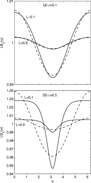
We have checked the perturbative solution by the numerical solution of the generalized differential equation. We find good agreement for small . For larger the numerical solution does not quite agree with the solution, as expected. Furthermore, we have been able to find smooth numerical solutions for a wide range of and . Figure 1 shows as a function of for two representative lengths and , with and . Solid lines are numerical solutions and dashed line are perturbative solutions. The case shows good agreement between the perturbative and numerical solutions. For the agreement is only qualitative.
3 Summary and Discussion
In summary, we have constructed an explicit counterexample to the assumption that potential fields remain potential under simple expansion or compression. For our 2D system, the reason that in general the field will not remain potential is quite simple. A potential field has to satisfy , which uniquely determines for the given boundary value of . This , however, has to satisfy an extra constraint to be self-consistent. That is, when substituting into the RHS of (6), we should get a constant. This is a very stringent constraint and in general will not be satisfied, as we have demonstrated with a simple example.
It should be pointed out that the domain under consideration is not compact, therefore specifying the normal component of the magnetic field on the boundary does not uniquely determine the potential field. One can, for example, add a constant or to the field without changing the normal component of . In this regard, our configuration does not belong to the same class of configurations as considered by Low et al. However, the purpose of this work is to demonstrate that a potential field can evolve into a non-potential field by simply changing the system length, therefore it should not be taken for granted that the final field has to remain potential. Since this is the key assumption in the demonstration of current singularity formation by Low et al., our findings suggest that their conclusion needs to be revisited. Furthermore, Eq. (22) shows that a parallel current is generated almost everywhere. This may account for why Low and coauthors find ubiquitous change in the footpoint mapping. Although our analytic demonstration of the existence of a smooth solution is based on perturbation theory, the demonstration is supported by numerical solution even when perturbation theory is not strictly valid.
The question posed by title “do potential fields develop current sheets under simple compression or expansion?” remains open at this point. Indeed, we cannot preclude the possibility that current sheets may form during the process. However, even if that is the case, a smooth current density is likely to precede the formation of current sheets. This raises the overall question as whether limiting to potential fields is a viable option in solving Parker’s problem. The answer is probably no.
References
- Antiochos (1987) Antiochos, S. K. 1987, Astrophys. J., 312, 886
- Craig & Sneyd (2005) Craig, I. J. D., & Sneyd, A. D. 2005, Solar Physics, 232, 41
- Grad et al. (1975) Grad, H., Hu, P. N., & Stevens, D. C. 1975, Proc. Natl. Acad. Sci., 72, 3789
- Janse & Low (2009) Janse, Å. M., & Low, B. C. 2009, Astrophys. J., 690, 1089
- Klimchuk (2006) Klimchuk, J. A. 2006, Solar Physics, 234, 41
- Longcope & Strauss (1994) Longcope, D. W., & Strauss, H. R. 1994, Astrophys. J., 437, 851
- Low (2006) Low, B. C. 2006, Astrophys. J., 649, 1064
- Low (2007) —. 2007, Phys. Plasmas, 14, 122904
- Marsh (1996) Marsh, G. E. 1996, Force-Free Magnetic Fields: Solutions, Topology and Applications (World Scientific)
- Ng & Bhattacharjee (1998) Ng, C. S., & Bhattacharjee, A. 1998, Phys. Plasmas, 5, 4028
- Parker (1972) Parker, E. N. 1972, Astrophys. J., 174, 499
- Parker (1979) —. 1979, Cosmical Magnetic Fields (Oxford University Press)
- Parker (1983) —. 1983, Astrophys. J., 264, 642
- Parker (1994) —. 1994, Spontaneous Current Sheets in Magnetic Fields (Oxford University Press, Inc.)
- Sturrock (1994) Sturrock, P. A. 1994, Plasma Physics: an Introduction to the theory of Astrophysical, Geophysical, and Laboratory Plasmas (Cambridge: Cambridge University Press)
- van Ballegooijen (1985) van Ballegooijen, A. A. 1985, Astrophys. J., 298, 421
- Zweibel & Li (1987) Zweibel, E. G., & Li, H.-S. 1987, Astrophys. J., 312, 423