Abstract

Given pseudo-random binary sequence of length $L$, assuming it consists of $k$ sub-sequences of length $N$. We estimate how $k$ scales with growing $N$ to obtain a limiting ergodic behaviour, to fulfill the basic definition of ergodicity (due to Boltzmann). The average of the consecutive sub-sequences plays the role of time (temporal) average. This average then compared to ensemble average to estimate quantitative value of a simple metric called Mean Ergodic Time (MET), when system is ergodic.

[Scaling of Ergodicity in Binary Systems]Scaling of Ergodicity in Binary Systems

M. Süzen

1 Introduction

Time averages play a central role in physics and statistical mechanics. An ergodic theorem provides a programme to compute ensemble averages of equilibrium properties of many component dynamics equivalently by taking time averages in the state-space [1, 2]. Hence, it is important to know when a dynamical system behave ergodically i.e. how long does it take to approach to the ergodic limit [3], in order to reliably use ergodic theorem and determine the averaged property in system where finding ensemble averages is not computationally feasible or not known a priori. Even finding ensemble averages is possible, covering the whole state-space may not be meaningful at all for the observable in consideration.

A particular system, the binary system is used to model many different physical or computational systems. While, it is quite simple in construction, measuring the ergodicity in this system via generating a large pseudo-random binary sequences essentially provides quantitative scaling measure.

2 Ensemble Average of a Binary System

Consider a binary sequence ${a_{j}},j=1,..,L$, each value in the sequence representing a state or a point in the phase-space, that can take two values $a_{j}\in{0,1}$, similar to a spin system [4].

For example, a set of ensemble of two state ($N=2$) binary system simply takes the following form: $\mathscr{S}=(00,11,10,01)$, and a binary sequence representing this is simply $00111001$. The length of this sequence $L$ is $8$, and the number of sub-sequences of length $N=2$ is $k=4$ (size of the set $\mathscr{S}$).

In general, using the values in each state indexed $i=1,..,N$, over different ensemble elements indexed $l=1,..,k$ (members within the set $\mathscr{S}$), ensemble average of each state $\langle A_{i}\rangle$ can be determined as follows:

$$\langle A_{i}\rangle=\frac{1}{k}\sum_{l=1}^{k}a_{l}^{i}.$$ (1)

Recall that $L,N,j,i,k\in\mathbb{Z}^{+}$ and for any state this ensemble average must be $1/2$ for a binary systems.

3 Measure of the Mean Ergodicity Time

If we generate a very long pseudo-random sequence that represents a temporal evolution (data) of the system, the average of each state is determined by a similar expression given in Equation (1), we call this value the time average. The estimate of the time (the number of sub-sequences, $k$) needed to reach vanishing difference in between the time average and ensemble average is called here the mean ergodicity time (MET) as a simple metric.

Since we are doing numerical experiments, defining a target metric of this difference is convenient. This metric $D_{MET}$ is defined as follows.

$$D_{MET}=\left|\langle A_{i}\rangle^{ensemble}-\langle A_{i}\rangle^{time}\right|.$$ (2)

When the difference reach to a vanishing value we record the number of sub-sequence ($k$ above) visited. Repeating this procedure will generate an estimate for the MET.

Using a reliable pseudo-random sequence is critical in determining averages of given number of states (sub-sequence blocks) in the ensemble (the whole sequence). We have used Mersenne Twister (MT) [5] that has a super astronomical period within the Maxima package [6] to generate a binary sequence. The measure of randomness and its quality in generated pseudo-random sequences discussed elsewhere in detail [7, 8].

$N$ state	Mean Ergodicity Time (MET)	Error	Number of Measurement
1	$685.5$	$343.41$	$60$
2	$29208.0$	$4416.15$	$373$
3	$194768.0$	$27747.53$	$87$
4	$249470.0$	$32428.54$	$56$
5	$343256.0$	$36243.63$	$70$
6	$517802.0$	$70089.40$	$33$

Table 1: Scaling of MET with increasing $N$ state. Number of Measurements mean the number of different ergodicaly behaving segments within the generated random sequence. Average length of these segments are defined to be MET.

The above procedure is nothing but to fulfill the basic definition of ergodicity. The computation of ensemble mean values of thermodynamic observable ($U$) [1] are multidimensional integrals over configuration space ${\bf x}$ [3],

$$\langle U\rangle=\int d{\bf x}P({\bf x})U({\bf x})$$

where $P({\bf x})$ is the probability of finding a system in the configuration ${\bf x}$. In principle, the arithmetic mean value $\bar{U}$, that is averaged over temporal evolution, must be equal to its ensemble mean value for a system in ergodic behaviour. The analogy of this definition for a binary system is given above.

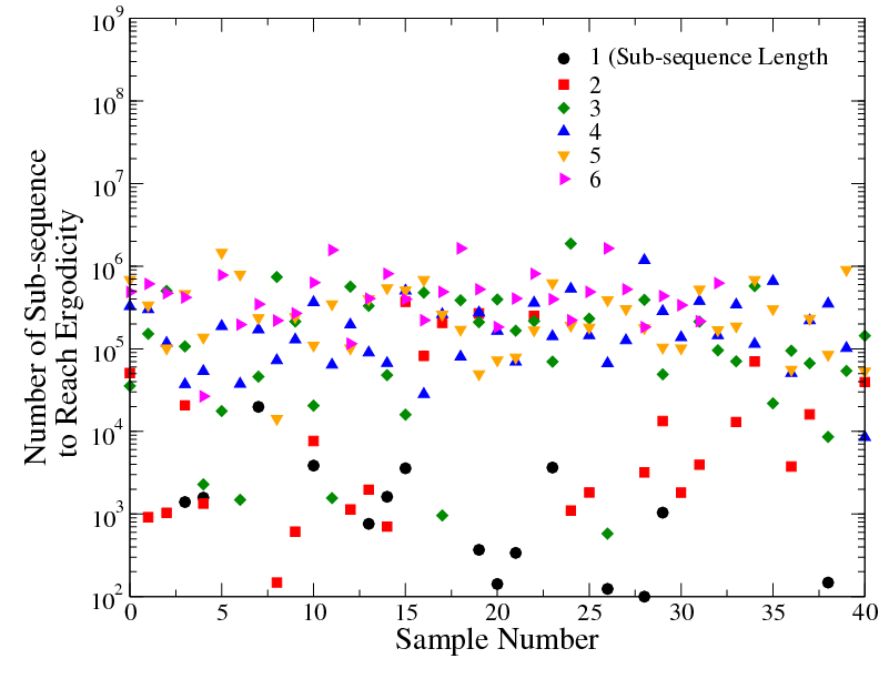
Figure 1: The sketch of measurements of the number of consecutive sub-sequences to reach ergodicity, the points where $D_{MET}$ metric reaches to value of $10^{-3}$.

4 Scaling of Ergodicity

We have measured number of sub-sequences ($k$) with increasing number of states (up to $N=6$). The measured MET and other details of the data is given in Table (1) and in Figure (1).

The scaling of MET against increasing number of states ($N$) is fitted in to an empirical law:

$$MET=\alpha\exp(\beta N^{\gamma}).$$ (3)

The scaling is shown in Figure (2). Where the value of scaling coefficients are found to be $\alpha=87.16$, $\beta=5.77$ and $\beta=0.227$. This scaling can be used to check when a binary system with large number of states reach to an ergodic behaviour.

5 Conclusions

A simple measure of scaling of ergodicity in binary systems, the length needed to reach ergodic behaviour with increasing system size, is explored by using a reliable pseudo-random binary sequence. Our result would help to determine a lower bound on how long an experiment on a binary system should be repeated until it reaches to a point to make averaging that is thermodynamically acceptable. The work presented here can also be used as a pedagogical tool in understanding ergodicity of a dynamical system.

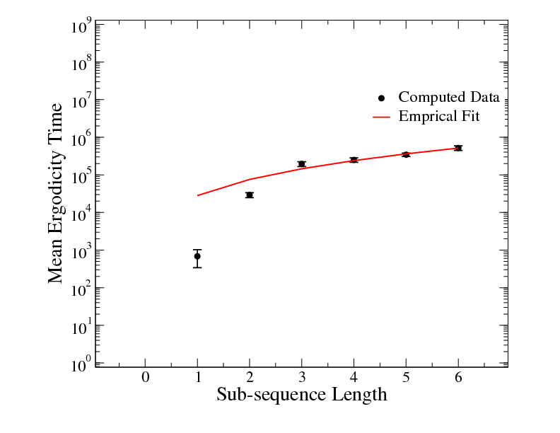
Figure 2: Scaling of ergodicity against the number of binary states (mimics the size of the state-space), averaged over many measurements summarized in Table (1), fitted to an empirical function curve given in Equation (3).

Appendix A Algorithm of MET measurements: Maxima Code

Here we present the Maxima code to generate the results. Note that given comments with a // are not valid Maxima syntax and must be removed in the actual code.

time_average(N,tolarence) := ( // N is the state size
    sub_unit:[], // initialize system
    sub_ave:[],
    for i:1 thru N step 1 do
    (
      sub_unit:append(sub_unit,[0]),  // assign dummy values initially
      sub_ave:append(sub_ave,[0])
    ),
      up:2, // initial upper bound for mean ergodicity time
    for i:1 thru up step 1 do
    (
     for j:1 thru N step 1 do
       (
         // populate system and collect for averages
           num:random(2), sub_unit[j]:sub_unit[j]+num
       ),
        sub_ave[1]:bfloat(sub_unit[1]/i), // initial time averages
        diff:abs(bfloat(0.5)-sub_ave[1]), //  and check
     for k:2 thru N step 1 do  // find out maximum difference
                               // between time average and ensemble averages
       (
        sub_ave[k]:bfloat(sub_unit[k]/i) ,
        tsub: sub_ave[k],
        difft:abs(bfloat(0.5)-sub_ave[k]),
        if difft > diff then diff:difft
       ),
      if diff >= tolarence then up:up+1 // increment for MET
                                       // otherwise algoritm stops
    ),
      print("",up), // Report MET
      print("#time_ave=",tsub) // and time average (must be close to 0.5)
);

References

- [1] R. C. Tolman. The Principles of Statistical Mechanics. Oxford U.P., New York, 1938.
- [2] I. E. Farquhar. Ergodic Theory in Statistical Mechanics. Interscience Publishers, Inc, New York, 1964.
- [3] J.P. Neirotti and David L. Freeman. Approach to ergodicity in monte carlo simulations. Physical Review E, 62(5):7445, 2000.
- [4] C. Kittel and H. Kroemer. Thermal Physics. W.H.Freeman and Company, 1980.
- [5] M. Matsumoto and T. Nishimura. Mersenne twister: A 623-dimensionally equidistributed uniform pseudo-random number generator. ACM Transactions on Modeling and Computer Simulation, 8(1):3–30, 1998.
- [6] http://maxima.sourceforge.net.
- [7] Aaldert Compagner. Definition of randomness. American Journal of Physics, 59(8):700, 1991.
- [8] W. Janke. Pseudo random numbers: Generation and quality checks. Quantum Simulations of Complex Many-Body Systems: from Theory to Algorithms, page 447, 2002.