Green-Function-Based Monte Carlo Method for Classical Fields Coupled to Fermions

Abstract

Microscopic models of classical degrees of freedom coupled to non-interacting fermions occur in many different contexts. Prominent examples from solid state physics are descriptions of colossal magnetoresistance manganites and diluted magnetic semiconductors, or auxiliary field methods for correlated electron systems. Monte Carlo simulations are vital for an understanding of such systems, but notorious for requiring the solution of the fermion problem with each change in the classical field configuration. We present an efficient, truncation-free $O(N)$ method on the basis of Chebyshev expanded local Green functions, which allows us to simulate systems of unprecedented size $N$.

The numerical simulation of quantum lattice models is a key tool in solid state research and many other fields of physics. One class of problems, which is notoriously difficult to study, are fermions coupled to classical degrees of freedom. Such microscopic models can arise if parts of a complex system are approximated classically. A prominent example is the double-exchange model, which describes the ferromagnetism of mixed-valence manganites on the basis of classical $t_{2g}$-spins whose orientation affects the kinetic energy of $e_{g}$ valence electrons. Zener (1951); Anderson and Hasegawa (1955); de Gennes (1960) Another example are Mn-doped (III,V) semiconductors, where itinerant holes trigger a ferromagnetic ordering of the Mn spins. Schliemann et al. (2001) A completely different route that leads to a coupling of fermions and classical degrees of freedom are the auxiliary field methods, which tackle the problem of interacting fermions. Here, a Hubbard-Stratonovich transformation is used to decouple the two-body interaction into non-interacting fermions in an auxiliary field, which is summed over with Monte Carlo methods. Blankenbecler et al. (1981); Hirsch and Fye (1986)

For all these systems the cause of the numerical difficulty is the requirement for a solution of the non-interacting fermion problem whenever the classical field is varied in a Monte Carlo simulation. We propose an efficient local-update algorithm, which obtains the change in fermionic energy directly from a few local Green functions. These Green functions can easily be calculated by Chebyshev expansion, superseding estimates of the density of states and thus trace calculations. We illustrate the efficiency of the approach with simulations of the double-exchange model.

The models we consider in this work are of the general form

$$H=\sum_{ij}c_{i}^{\dagger}A_{ij}(\vec{\phi})c_{j}\,,$$ (1)

where $c_{i}^{(\dagger)}$ are fermion creation (annihilation) operators at lattice site $i$, and $\vec{\phi}$ is a classical field with one or more components at each site. For example, the double-exchange model Kogan and Auslender (1988); Weiße et al. (2001) is given by the Hamiltonian

$$H=-\sum_{\langle ij\rangle}t_{ij}c_{i}^{\dagger}c_{j}\,,$$ (2)

where the summation is over nearest-neighbor sites and the hopping $t_{ij}$ depends on the orientation $\{\theta_{i},\phi_{i}\}$ of classical local spins at each site,

$$t_{ij}=\cos\tfrac{\theta_{i}-\theta_{j}}{2}\cos\tfrac{\phi_{i}-\phi_{j}}{2}+\operatorname{i}\cos\tfrac{\theta_{i}+\theta_{j}}{2}\sin\tfrac{\phi_{i}-\phi_{j}}{2}\,.$$ (3)

This complex matrix element is one for ferromagnetically aligned spins and vanishes for anti-ferromagnetic alignment. At low temperature the system favors ferromagnetism, since it can gain kinetic energy.

The thermodynamics is described by the partition function

$$Z=\operatorname{Tr}_{\text{c}}\operatorname{Tr}_{\text{f}}\exp[-\beta(H(\vec{\phi})-\mu N)]$$ (4)

and its derivatives. Here the traces $\operatorname{Tr}_{\text{c}}$ and $\operatorname{Tr}_{\text{f}}$ sum over the classical and fermionic degrees of freedom, respectively. The fermionic trace can be rewritten in terms of the single-particle eigenvalues $\epsilon_{i}$ of $H$,

$$Z=\operatorname{Tr}_{\text{c}}\exp[-S_{\text{eff}}(\vec{\phi})]\,,$$ (5)

such that the grand potential of the fermions times $\beta$,

$$S_{\text{eff}}(\vec{\phi})=-\sum_{i}\log\big{(}1+\exp[-\beta(\epsilon_{i}(\vec{\phi})-\mu)]\big{)}\,,$$ (6)

defines an effective Euclidean action for the classical degrees of freedom. The second trace over the classical field can then be calculated with a standard Monte Carlo sampling, where the weight of a configuration $\vec{\phi}$ is given by

$$P(\vec{\phi})=\exp[-S_{\text{eff}}(\vec{\phi})]/Z\,.$$ (7)

However, a non-trivial problem remains: To calculate $P(\vec{\phi})$ we need to know the spectrum $\{\epsilon_{i}\}$ of the non-interacting fermion system, or at least its change under a proposed Monte Carlo update $\vec{\phi}\to\vec{\phi}^{\prime}$.

There are different solutions to this problem: We could use brute force and calculate all eigenvalues of $A_{ij}(\vec{\phi})$ whenever $\vec{\phi}$ is modified. For local update schemes this is, of course, very expensive and imposes severe restrictions on the accessible system sizes. As a way out, hybrid approaches Scalettar et al. (1986); Duane et al. (1987); Alonso et al. (2001); Weiße et al. (2005) have been suggested, where updates of the whole field configuration are calculated with an approximate dynamics. Then, the solution of the full fermion problem in the acceptance step is required less frequently. However, if the approximate dynamics does not closely match the exact one, the acceptance rate drops markedly, in particular for increased system size. Therefore, these approaches crucially depend on the quality of the approximate action.

Staying with local updates of the classical field one can try to optimize the calculation of the fermion spectrum. Motome and Furukawa Motome and Furukawa (1999, 2000, 2001) suggested a Chebyshev expansion of the fermion density of states, which can be calculated with an effort proportional to the square of the system size $N$. A further modification Furukawa and Motome (2004); Alvarez et al. (2005), involving several truncations in the moment calculation, reduced the effort to order $N$.

In another recent approach Alvarez et al. (2007) the evolution of the eigenvalues of $A_{ij}(\vec{\phi})$ under small local changes of $\vec{\phi}$ is tracked using special techniques for low-rank matrix updates Golub and van Loan (1996). Then again, the full solution of the fermion problem is required only occasionally. In the best case this leads to $N\log N$ scaling.

In the present work we combine ideas from the last two approaches and directly calculate the change of the fermion density of states using a few real space Green functions. Relying on Chebyshev expansion these can be calculated with an effort proportional to the system size $N$. Without any truncations we arrive at an order-$N$ algorithm.

Let us start from the Hamiltonian $H$ with the Hermitian hopping matrix $A$ and ask how the spectrum changes, when a local modification $\Delta$ is added. Given $a(E)=A-E\mathbb{1}$ and its inverse $G(E)$, i.e. the Green function with $G(E)a(E)=\mathbb{1}$, the spectrum of $A+\Delta$ follows from

$$(A+\Delta)|\psi\rangle =E|\psi\rangle\,,$$ (8)

$$(a(E)+\Delta)|\psi\rangle =0\,.$$

Right multiplication with $G(E)$ yields

$$G(E)(a(E)+\Delta)|\psi\rangle=(\mathbb{1}+G(E)\Delta)|\psi\rangle=0\,.$$ (9)

The spectrum of $A+\Delta$ is given by those values of $E$ where the determinant

$$d(E):=\det(\mathbb{1}+G(E)\Delta)$$ (10)

vanishes. Recalling introductory lectures on Green functions (see e.g. Ref. Ziman, 1972) we note that this $N$-dimensional determinant reduces to one with a dimension equal to the rank of $\Delta$. For local Monte Carlo updates this is a small number. If we change, for instance, the on-site potential, $\Delta$ has a single non-zero matrix element and we merely need the local Green function of the corresponding site. For the double exchange model a single spin flip affects the hopping between the site and its nearest neighbors. Independent of the system size $N$ or the space dimension, Eq. (10) then reduces to a $2\times 2$ problem, i.e., we need only four Green functions connecting the site with its environment and both to themselves.

Before we go into the details of calculating $d(E)$, let us further analyze the meaning of this quantity. Going back to Eq. (9) we have

$$d(E) =\det[G(E)(a(E)+\Delta)]$$ (11)

$$=\det[G(E)]\det[a(E)+\Delta]\,.$$

This can be expressed in terms of the eigenvalues $\{\epsilon_{i}\}$ of $A$ and $\{\epsilon_{i}^{\prime}\}$ of $A+\Delta$,

$$d(E)=\prod_{i}\frac{1}{\epsilon_{i}-E}\prod_{i}(\epsilon_{i}^{\prime}-E)\,.$$ (12)

An important trick of our new approach consists of going to the complex plane, $E\to z:=E+\operatorname{i}\varepsilon$, and taking a logarithmic derivative. We now observe that $d(E)$ determines exactly what we need for the Monte Carlo update: the change in the density of states going from $A$ to $A+\Delta$, i.e., from $\vec{\phi}$ to $\vec{\phi}^{\prime}$,

$$\frac{1}{\pi}\operatorname{Im}\lim_{\varepsilon\to 0}\frac{d\log(d(z))}{dz} =\frac{1}{\pi}\operatorname{Im}\lim_{\varepsilon\to 0}\sum_{i}\frac{1}{\epsilon_{i}-z}-\frac{1}{\epsilon_{i}^{\prime}-z}$$ (13)

$$=\sum_{i}\delta(\epsilon_{i}-E)-\delta(\epsilon_{i}^{\prime}-E)$$

$$=\rho(E)-\rho^{\prime}(E)\,.$$

The change in the effective action then reads

$$S_{\text{eff}} (\vec{\phi}^{\prime})-S_{\text{eff}}(\vec{\phi})=$$ (14)

$$=\int\log(1+\operatorname{e}^{-\beta(E-\mu)})(\rho(E)-\rho^{\prime}(E))dE$$

$$=\frac{\beta}{\pi}\int\frac{1}{1+\operatorname{e}^{\beta(E-\mu)}}\operatorname{Im}\lim_{\varepsilon\to 0}\log(d(E+\operatorname{i}\varepsilon))dE\,,$$

where in the last line partial integration led to an integral over the Fermi function. The key role of $d(z)$ has already been noted earlier Fucito et al. (1981); Scalapino and Sugar (1981), but the evaluation of Eq. (10) becomes feasible only if we can restrict ourselves to a minimal set of Green functions and an efficient, direct method for their calculation.

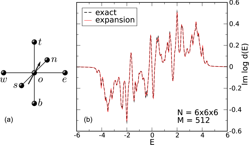
Figure 1: (color online). (a) Labeling of the nearest neighbor sites on a cubic lattice. (b) Comparison of $\operatorname{Im}\log(d(E+\operatorname{i}\varepsilon))$ calculated from exact eigenvalues $\epsilon_{i}$, $\epsilon_{i}^{\prime}$ and with Chebyshev expansion of order $M=512$ ($\varepsilon=0.0625$) for a $6^{3}$ site sample.

Let us now explain this main part of our new approach for the double exchange model on a cubic lattice. Here, a local update consists of rotating a single spin at a site $o$. This modifies the matrix element $t_{ij}$ between $o$ and its nearest neighbors to the north, east, south, and so on. Labeling the sites according to Fig. 1(a), a naïve evaluation of Eq. (10) requires all $7\times 7$ Green functions $G_{ij}(z)$ with $i,j\in\{o,n,e,s,w,t,b\}$ rem . However, we can do much better observing that

$$d(z) =\det(\mathbb{1}+G(z)\Delta)$$ (15)

$$=[1+\sum_{j\in\text{n.n.}}\Delta_{jo}G_{oj}(z)][1+\sum_{j\in\text{n.n.}}\Delta_{oj}G_{jo}(z)]$$

$$-G_{oo}(z)[\sum_{j,k\in\text{n.n.}}\Delta_{jo}\Delta_{ok}G_{kj}(z)]$$

can be expressed in terms of only $2\times 2$ Green functions,

$$d(z)=[1+G_{ov}(z)][1+G_{vo}(z)]-G_{oo}(z)G_{vv}(z)\,,$$ (16)

which connect the original site $o$ and the environment state

$$|v\rangle=\Delta|o\rangle=\sum_{j\in\text{n.n.}}\Delta_{jo}|j\rangle\,.$$ (17)

All four Green functions can be calculated easily with the Chebyshev expansion approach outlined in a recent review Weiße et al. (2006). In a nutshell, diagonal elements $G_{ii}(z)$ are expanded in terms of the Chebyshev polynomials of first and second kind, $T_{m}$ and $U_{m}$, respectively,

$$G_{ii}(E+\operatorname{i}\varepsilon)=\frac{\operatorname{i}[\mu_{0}+2\sum_{m=1}^{M-1}\mu_{m}T_{m}(E/s)]}{\sqrt{s^{2}-E^{2}}}\\ +2\sum_{m=1}^{M-1}\mu_{m}U_{m-1}(E/s)\\ =\operatorname{i}\frac{\mu_{0}+2\sum_{m=1}^{M-1}\mu_{m}\exp[-\operatorname{i}m\arccos(E/s)]}{\sqrt{s^{2}-E^{2}}}\,.$$ (18)

The expansion coefficients $\mu_{m}$ are Chebyshev moments modified by appropriate kernel factors, which improve the convergence of the truncated series and damp Gibbs oscillations,

$$\mu_{m}=\langle i|T_{m}(H/s)|i\rangle\frac{\sinh[\lambda(1-m/M)]}{\sinh\lambda}\,.$$ (19)

The scaling factor $s$ ensures that the spectrum of the Hamiltonian $H/s$ falls within the domain of the Chebyshev polynomials $[-1,1]$. For the double exchange model we can choose $s$ to be a little larger than the bare bandwidth in the ferromagnetic case, $s>6$. The kernel parameter $\lambda$ regulates the resolution of the method versus the damping of Gibbs oscillations. A good value is $\lambda=4$. The resolution at which the Green function is approximated is given by $\varepsilon=\lambda s/M$. The limit $\varepsilon\to 0$ thus corresponds to infinite expansion order $M$. In a numerical simulation, of course, $M$ is always finite and we need to extrapolate data for different $M$ to obtain the limiting value of $S_{\text{eff}}(\vec{\phi}^{\prime})-S_{\text{eff}}(\vec{\phi})$. Since in Eq. (14) we integrate a function of $G_{ij}(z)$ over the Fermi function, the maximal resolution should be better than the thermal broadening of the Fermi step, which is of the order of $1/\beta$. Low temperatures, therefore, require higher expansion orders.

The most time consuming step of the whole simulation is the calculation of the moments $\langle i|T_{m}(H/s)|i\rangle$. Using the recursion relation

$$T_{m}(x)=2xT_{m-1}(x)-T_{m-2}(x)$$ (20)

it reduces to sparse matrix-vector multiplications, the cost of which scales linearly with the system size $N$. With a further trick based on

$$T_{2m+i}=2T_{m}T_{m+i}-T_{i}\quad\text{with}\quad i=0,1$$ (21)

we obtain two moments per matrix-vector multiplication. Moreover, half of the moments vanish due to the relation $|v\rangle=\Delta|o\rangle$ and the special structure of the Chebyshev recursion (20).

At this point we should also note the advantage over approaches based on a full expansion of the density of states: For the latter the moments are given by traces, $\mu_{m}\sim\operatorname{Tr}\{T_{m}(H/s)\}$, instead of simple expectation values. Unless truncated or otherwise approximated Furukawa and Motome (2004), their calculation requires $O(N^{2})$ operations.

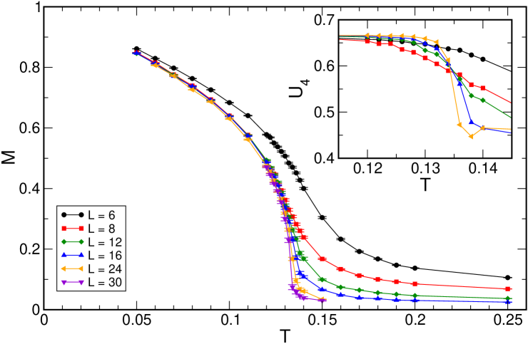
Figure 2: (color online). Main panel: Magnetization versus temperature for the double-exchange model on 3D clusters with periodic boundary conditions ($N=L^{3}$). Inset: Binder ratio $U_{4}$ showing a crossing near $T\approx 0.134$.

So far we have discussed only the diagonal Green functions $G_{ii}$. In Ref. Weiße et al., 2006 we showed that symmetric Green functions $G_{ij}=G_{ji}$ can be expanded in the same manner. However, in the double exchange model the spins induce local magnetic fields which break this symmetry. We therefore derive the off-diagonal Green functions $G_{ov}$ and $G_{vo}$ from the two diagonal functions $G_{o+v,o+v}$ and $G_{o+\operatorname{i}v,o+\operatorname{i}v}$. With all required moments at hand we can evaluate the sums in Eq. (18) with fast Fourier methods, calculate $d(E)$ with Eq. (16), and finally integrate over the Fermi function to obtain the change of $S_{\text{eff}}$. In Fig. 1(b) we show a typical example of $\operatorname{Im}\log(d(E+\operatorname{i}\varepsilon))$ and compare the expansion with the exact result from a full diagonalization.

Having explained the technical details of the approach let us now illustrate its applicability with a few results for the double-exchange model (2) at half filling, $\mu=0$. In the main panel of Fig. 2 we show the magnetization as a function of temperature, where the latter is measured in units of the maximal hopping amplitude $t\equiv 1$. As expected, we observe a phase transition to a ferromagnetically ordered phase below $T\approx 0.14$. A closer inspection based on the Binder parameter Binder (1981)

$$U_{4}=1-\frac{\langle m^{4}\rangle}{3\langle m^{2}\rangle^{2}}$$ (22)

yields the estimate $T_{c}\approx 0.134$, see the inset of Fig. 2. This agrees with previous estimates Motome and Furukawa (2001); Alonso et al. (2001); Motome and Furukawa (2003) of the critical temperature, which range between 0.128 and 0.139.

The data in Fig. 2 is based on expansions of order $M=256$ and averages over 6000 to 20000 Monte Carlo steps in the critical region, where one step corresponds to $N$ spin flips. It is the low resource consumption which allows for these far more precise calculations compared to previous studies Motome and Furukawa (2001, 2003), which were based on Chebyshev expansions of order $M\approx 20$. Note also that we can handle much larger systems with $N=30^{3}$ sites, i.e. a complex matrix dimension of $27000$.

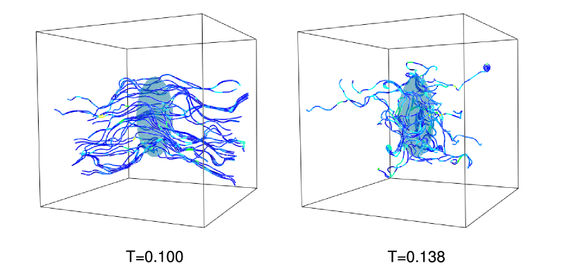
Figure 3: (color online). Structure of the 3D spin field at two different temperatures visualized with stream lines.

To visualize the spatial structure of the spin field we imagine it as a liquid flow and draw curves tangent to the velocity field. These stream lines are regular and parallel in the ordered phase, but quite irregular and swirled near and above the phase transition, see Fig. 3. Of course, this visualization method fails for truly disordered spin fields.

In summary, we have presented an efficient local update scheme for Monte Carlo simulations of classical fields coupled to fermions. At the core of the approach is an expression which relates the change of the fermion spectrum to a few local Green functions. These can be calculated easily with Chebyshev expansion. Compared to similar expansion approaches a full trace over the fermion system is spared, which directly leads to a fast and precise order-$N$ algorithm. Possibly our method can be further accelerated using the approximations inherent in the truncated polynomial expansion method Furukawa and Motome (2004); Alvarez et al. (2005). The calculations presented were performed on the TeraFLOPS cluster of the Institute for Physics at Greifswald university.

References

- Zener (1951) C. Zener, Phys. Rev. 82, 403 (1951).
- Anderson and Hasegawa (1955) P. W. Anderson and H. Hasegawa, Phys. Rev. 100, 675 (1955).
- de Gennes (1960) P.-G. de Gennes, Phys. Rev. 118, 141 (1960).
- Schliemann et al. (2001) J. Schliemann, J. König, and A. H. MacDonald, Phys. Rev. B 64, 165201 (2001).
- Blankenbecler et al. (1981) R. Blankenbecler, D. J. Scalapino, and R. L. Sugar, Phys. Rev. D 24, 2278 (1981).
- Hirsch and Fye (1986) J. E. Hirsch and R. M. Fye, Phys. Rev. Lett. 56, 2521 (1986).
- Kogan and Auslender (1988) E. M. Kogan and M. I. Auslender, Phys. Status Solidi B 147, 613 (1988).
- Weiße et al. (2001) A. Weiße, J. Loos, and H. Fehske, Phys. Rev. B 64, 054406 (2001).
- Scalettar et al. (1986) R. T. Scalettar, D. J. Scalapino, and R. L. Sugar, Phys. Rev. B 34, 7911 (1986).
- Duane et al. (1987) S. Duane, A. Kennedy, B. J. Pendleton, and D. Roweth, Phys. Lett. B 195, 216 (1987).
- Alonso et al. (2001) J. L. Alonso, L. A. Fernández, F. Guinea, V. Laliena, and V. Martín-Mayor, Nucl. Phys. B 596, 587 (2001).
- Weiße et al. (2005) A. Weiße, H. Fehske, and D. Ihle, Physica B 359–361, 702 (2005).
- Motome and Furukawa (1999) Y. Motome and N. Furukawa, J. Phys. Soc. Jpn. 68, 3853 (1999).
- Motome and Furukawa (2000) Y. Motome and N. Furukawa, J. Phys. Soc. Jpn. 69, 3785 (2000).
- Motome and Furukawa (2001) Y. Motome and N. Furukawa, J. Phys. Soc. Jpn. 70, 3186 (2001), erratum.
- Furukawa and Motome (2004) N. Furukawa and Y. Motome, J. Phys. Soc. Jpn. 73, 1482 (2004).
- Alvarez et al. (2005) G. Alvarez, C. Sen, N. Furukawa, Y. Motome, and E. Dagotto, Comp. Phys. Comm. 168, 32 (2005).
- Alvarez et al. (2007) G. Alvarez, P. K. V. V. Nukala, and E. D’Azevedo, J. Stat. Mech. p. P08007 (2007).
- Golub and van Loan (1996) G. H. Golub and C. F. van Loan, Matrix Computations (Johns Hopkins University Press, Baltimore, 1996), 3rd ed.
- Ziman (1972) J. M. Ziman, Principles of the Theory of Solids (Cambridge University Press, Cambridge, 1972), 2nd ed.
- Fucito et al. (1981) F. Fucito, E. Marinari, G. Parisi, and C. Rebbi, Nucl. Phys. B 180, 369 (1981).
- Scalapino and Sugar (1981) D. J. Scalapino and R. L. Sugar, Phys. Rev. Lett. 46, 519 (1981).
- (23) In Ref. Scalapino and Sugar, 1981 this is described as a reduction to a problem.
- Weiße et al. (2006) A. Weiße, G. Wellein, A. Alvermann, and H. Fehske, Rev. Mod. Phys. 78, 275 (2006).
- Binder (1981) K. Binder, Z. Phys. B 43, 119 (1981).
- Motome and Furukawa (2003) Y. Motome and N. Furukawa, J. Phys. Soc. Jpn. 72, 2126 (2003).