LAPTH-1325/2009
The Thermal Abundance of Semi–Relativistic Relics
Manuel Drees***drees@th.physik.uni-bonn.de, Mitsuru Kakizaki†††kakizaki@lapp.in2p3.fr and Suchita Kulkarni‡‡‡kulkarni@th.physik.uni-bonn.de
aPhysikalisches Institut and
Bethe Center for Theoretical Physics,
Universität Bonn,
D-53115 Bonn, Germany
bLAPTH, Université de Savoie, CNRS,
B.P. 110, F-74941 Annecy-le-Vieux Cedex, France
1 Introduction
The accurate determination of cosmological parameters by up–to–date observations, most notably by the Wilkinson Microwave Anisotropy Probe (WMAP) [1], increases the importance of quantitative predictions. In particular, the estimate of the cosmological relic abundances of particle species is essential, for the history of the universe depends on these quantities. One of the most important examples is the cosmological abundance of dark matter [2, 3], whose mass density is found to be [1]
| (1) |
where is the scaled Hubble parameter in units of and is the mass density in units of the critical density.
The abundance of some particle species is determined by solving the Boltzmann equation, which describes the change of the particle number caused by particle reactions as well as by the expansion of the universe [2]. However, there is no analytical general solution of this nonlinear differential equation, and therefore one needs to solve the equation numerically in many cases. In early studies, approximate analytical formulae have been found for the relativistic [4, 2] and non-relativistic [5, 6, 7] regimes.
Stable or long–lived weakly interacting massive particles (WIMPs) with weak–scale masses are examples of cold relic particles, which decouple from thermal equilibrium when they are non–relativistic. In standard cosmology, decoupling of WIMPs occurs in the radiation–dominated (RD) era after inflation, and analytic approximate formulae for the WIMP relic abundance have been derived [5, 6, 7]. In the opposite limit, where decoupling of particles from the thermal background occurs when they are relativistic, the relic abundance is approximated by its equilibrium value at the decoupling temperature, and not sensitive to details of its freeze–out [2]. The resulting relic density can therefore easily be computed analytically. On the other hand, no analytical treatment to calculate the relic abundance in the intermediate regime is known yet.
In this paper, we revisit the relic density of particles that decouple from the thermal bath when they were semi–relativistic, i.e. at freeze–out temperature . Assuming that the Maxwell–Boltzmann distribution can be used for all participating particles, we introduce an expression for the thermal average of the annihilation cross section which smoothly interpolates between the extremely relativistic and non–relativistic regimes. It is shown that our new ansatz is capable of reproducing the exact thermally–averaged annihilation cross section with accuracy of a few percent. Given this approximated cross section, we can define the freeze–out temperature by comparing the annihilation rate to the expansion rate. The assumption that the comoving density remains constant after freeze–out turns out to be a good approximation for the relic abundance of semi–relativistic particles.
We also discuss the roles such semi–relativistic particles could play in realistic cosmological scenarios. It should be emphasized that the abundance of semi–relativistically decoupled relics tends to be large because it is only very mildly Boltzmann suppressed. We point out that scenarios where semi–relativistically decoupling particles form the Dark Matter have problems with structure formation, Big Bang Nucleosynthesis (BBN) and/or laboratory measurements. Nevertheless, such semi–relativistic relics can be useful for diluting the density of other, unwanted relics by late–time out–of–equilibrium decay [8, 9]. As an example, we investigate a scenario of decaying sterile neutrino that is assumed to depart from thermal equilibrium when it is semi–relativistic, in sharp contrast to non–thermal sterile neutrino scenarios [10]. Thermal equilibrium is attained by introducing some higher–dimensional operator. It is illustrated that an enormous amount of entropy can be produced without spoiling the successful BBN prediction of the light element abundances.
This paper is organized as follows: In Sec. 2 we begin by reviewing briefly the method to calculate relic densities for relativistic and non–relativistic particles. In Sec. 3 we explain the new formalism which is applicable for all freeze–out temperatures in case of – and –wave cross sections. The way to calculate the freeze–out temperature is also shown. In Sec. 4, the possibility for semi-relativistic particles to have the observed dark matter relic density of is considered. Then, we discuss the amount of entropy produced by the decay of unstable semi–relativistic species that decay in less than a second. Finally, Sec. 6 is devoted to summary and conclusions. Some properties of modified Bessel functions are described in Appendix A. In Appendix B we argue that the use of the Maxwell–Boltzmann distribution in the definition of the thermally averaged cross section only leads to a small mistake in the final relic density.
2 Relic abundances in the non–relativistic and relativistic limits
In this Section we briefly review the standard analytical approximations for evaluating the relic abundance of hypothetical particles [2, 5, 7]. These are applicable to particles that were either non–relativistic or extremely relativistic at freeze–out.
The number density is obtained by solving the corresponding Boltzmann equation [2]. For the moment, we assume that single production and decay are forbidden by some symmetry or adequately suppressed. The Boltzmann equation takes a simple form if one further assumes that the quantum statistics factors describing the Bose enhancement or Fermi suppression of all final states can be neglected; in Appendix B it is shown that this is essentially equivalent to assuming that the distribution functions of all relevant particles are proportional to the Maxwell–Boltzmann distribution. The Boltzmann equation for can then be written as [2]
| (2) |
where is the equilibrium number density, is the thermal average of the annihilation cross section multiplied by the relative velocity between the two annihilating particles, and is the Hubble expansion rate of the universe. The second term on the left–hand side describes the dilution caused by the expansion of the universe; the first (second) term on the right–hand side decreases (increases) the number density due to annihilation into (production from) other particles, which are assumed to be in complete thermal equilibrium.
It is useful to express the above Boltzmann equation in terms of the dimensionless quantities and . The entropy density is given by , with being the effective number of relativistic degrees of freedom and the temperature of the universe. We also introduce the dimensionless ratio of mass to the temperature, . Assuming an adiabatic expansion of the universe, Eq.(2) can then be rewritten as [2]
| (3) |
The generic picture of decoupling from the thermal bath is as follows. After inflation, the universe becomes radiation–dominated with expansion rate
| (4) |
where GeV is the reduced Planck mass. The reheat temperate is assumed to be high enough for particles to reach full thermal (chemical as well as kinetic) equilibrium.***The case where the reheat temperature is too low for to attain chemical equilibrium has been discussed in [11, 12]. Thermal equilibrium is maintained as long as the interaction rate is larger than the Hubble expansion rate . As the temperature decreases, the interaction rate decreases more rapidly than the expansion rate does. When the interaction rate falls below the expansion rate, is no longer kept in thermal equilibrium and the comoving number density becomes essentially constant. This transition temperature is referred to as the freeze–out temperature .
Analytical expressions for the resulting relic density are known for the cases where decoupling happens when is non–relativistic or relativistic . We discuss these two limiting cases in the following Subsections.
2.1 Relativistic case
First, consider the case where particles decouple when they are ultra–relativistic (). In this case the equilibrium number density to entropy ratio depends on the temperature only through the number of degrees of freedom of the thermal bath. Therefore, the final relic abundance is to very good approximation equal to its equilibrium value at the time of decoupling:
| (5) |
where
| (8) |
with being the number of internal (e.g., spin or color) degrees of freedom of . Following the conventional notation, we express the relic density as , where is the present critical density of the universe, and is the present entropy density. This yields
| (9) |
It should be noted that the relic density is simply proportional to the mass of the particle in the relativistic case.
2.2 Non–relativistic case
For the non–relativistic case where , the relic abundance strongly depends on the freeze–out temperature because the equilibrium abundance is exponentially suppressed as the temperature decreases. The temperature dependence of the thermal average of the annihilation cross section is obtained using the Taylor expansion in powers of the velocity squared:
| (10) |
The numerically–evaluated correct relic abundance is reproduced with an accuracy of a few percent using the approximate analytic formula
| (11) |
For WIMPs with electroweak scale mass, freeze-out occurs at . The corresponding scaled relic density is then given by
| (12) |
Note that the relic density of a non–relativistic particle is inversely proportional to its annihilation cross section, but does not depend explicitly on its mass.
3 Abundance of semi–relativistically decoupling particles
In the previous Section, we reviewed the known relativistic and non–relativistic approximate formulae for the relic abundance. The main aim of this Section is to find a simple method applicable between the two regimes: an analytic estimate of the relic abundance of semi–relativistically decoupling particles ().
One of the key quantities that determine the freeze–out temperature is the thermally–averaged cross section. In the non–relativistic case, expressions for the equilibrium number density as well as for the thermally–averaged cross section times velocity are rather simple. For a semi–relativistic particle, however, the thermally–averaged cross section involves multiple integrals and cannot be expanded with respect to the velocity nor to the mass. Here we discuss a method of approximating the thermally-averaged cross section, by interpolating between its relativistically and non–relativistically expanded expressions. We employ the Maxwell–Boltzmann distribution for the equilibrium number density [7]:
| (13) |
The thermal average of the cross section is then obtained as [7]
| (14) |
where and is the first and second modified Bessel function of the second kind; some properties of these functions are given in Appendix A.
At first glance the use of the Maxwell–Boltzmann distribution seems improper for particles that are semi–relativistic at decoupling, let alone for ultra–relativistic particles. However, we will argue in Appendix B that this should still yield accurate results for the final relic density. This is partly due to cancellations between the numerator and denominator of Eq.(14), and partly due to the fact that the final result for becomes less sensitive to as decreases.
As examples of the annihilation of particles, we consider the pair annihilation processes of Dirac and Majorana fermions (e.g. neutrinos) into a pair of massless fermions, [4, 13, 14]. It should, however, be noticed that this assumption includes more general cases of any other species annihilating from or wave initial states. In a renormalizable model, the annihilation is mediated by some heavy particle: for example, a –boson with tiny coupling with , or a new spin- boson [15]. We assume that the mass of this exchange particle is much larger than , so that the annihilation amplitude can be described through an effective four–fermion interaction.
The annihilation of two Dirac fermions proceeds from an wave, and the resulting cross section can be parameterized as
| (15) |
where is the center–of–mass energy squared. denotes the coupling constant of the four–fermion interaction (e.g. the Fermi coupling constant, GeV-2). Finally, is the relative velocity defined as
| (16) |
where and are the four–momenta and energies of the two incident particles labeled and . The resulting thermally averaged cross section is given by
| (17) | |||||
Its relativistic and non–relativistic limits read
| (18) |
respectively. A general expression for should reproduce these results for and , respectively. A simple possibility is
| (19) |
It should be noticed that this choice is not unique.
Let us turn to the case of the annihilation from a wave initial state, which is e.g. true if is a Majorana fermion. Eq.(15) should then be replaced by
| (20) |
Thermal averaging leads to
| (21) | |||||
Following the same steps as in the wave case, we find the following interpolation:
| (22) |
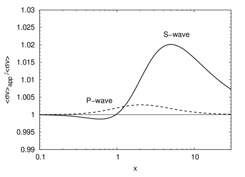
Figure 1 shows the ratio of the approximate to the exact cross section for the (solid line) and wave (dashed) cases. Note that this ratio depends only on . We see that our approximate expressions reproduce the exact ones with accuracy of better than 2% (0.5%) for annihilation from an ()wave, even in the semi–relativistic region ().
Using Eqs.(19) or (22) instead of the exact expressions (17) or (21) greatly reduces the numerical effort required to solve the Boltzmann equation (3). At the cost of some further loss of accuracy, an even faster estimate of the relic density can be obtained by using an approximate solution of the Boltzmann equation instead of the accurate evaluation of the relic abundance by solving the Boltzmann equation numerically. The determination of the temperature where some interaction decouples plays an important role in the analytical prediction of the relic abundance. Indeed, for non–relativistically decoupling particles the relic abundance is sensitive to the freeze–out temperature because of the Boltzmann suppression. In this case, a rough estimate of obtained by equalizing the interaction rate and the Hubble expansion rate is not sufficient to make an accurate prediction. Here we show that for semi–relativistically decoupling particles a simple comparison of the interaction rate and the Hubble expansion rate still gives a reasonably accurate result for the final relic density.
We define the freeze–out temperature by equalizing the interaction rate and the Hubble expansion rate,†††This definition of the freeze–out temperature should not be used for the prediction of the relic abundance through Eqs.(11) and (12).
| (23) |
We then simply assume that does not change after decoupling from the thermal bath, so that
| (24) |
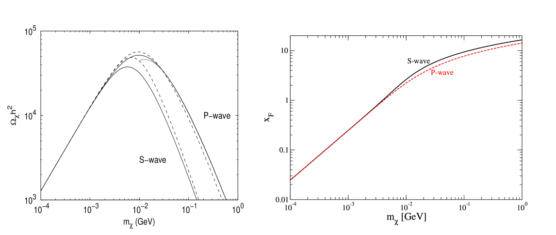
Let us see to what extent this method can reproduce the correct relic abundance. As an example, we consider the pair annihilation of neutrino–like particles via the mediation of the weak SM gauge bosons‡‡‡Our primary concern here is to test our approximation for the relic abundance, and thus, as an illustration, we take such an unrealistic setup.. In the left frame of Fig. 2 we plot the relic abundance as function of . The solid curves show predictions for the relic abundance obtained by solving the Boltzmann equation (3) numerically, while the dashed curves have been obtained using the analytic approximation described above. The upper curves are for Majorana fermions annihilating from a wave, and the lower curves are for Dirac fermions case annihilating from an wave. We take , and §§§Since we concentrate on the ratio of the exact to the approximate relic densities, we discard the temperature dependence of , which is basically an overall factor.. The right frame shows the corresponding values of .
This figure shows that our very simple analytical treatment reproduces the correct relic density with an error of at most 20% (5%) for semi–relativistically decoupling particles annihilating from an ()wave. Not surprisingly, our treatment becomes exact for particles that are relativistic at decoupling.¶¶¶We will see in Appendix B that one should use the correct Fermi–Dirac or Bose–Einstein expression for in Eq.(24) in order to accurately predict the relic density for . In the Dirac case, our approximation coincides with the exact relic abundance for GeV, corresponding to ; however, the deviation becomes larger again for larger . Therefore, our method is not applicable for the entire region of cold relics. Instead, one could switch to the usual non–relativistic treatment described in Sec. 2.2 at the cross–over value, i.e. at . In the wave case the cross–over already occurs at MeV, corresponding to . The dotted curve shows that the non–relativistic approximation is already quite reliable at this point. We can thus smoothly match our approximation to the usual non–relativistic treatment for both and wave annihilation.
4 Semi–relativistic dark matter?
As a first application, let us analyze whether semi–relativistically decoupled particles () can be a dark matter candidate, whose cosmological abundance should be . The final number density of such a particle is of order of . Combining this value with the observed amount of dark matter, the upper bound of the semi–relativistic particle turns out to be eV, which would thus decouple at temperatures of a few dozen eV. These particles would therefore still be ultra–relativistic during the formation of 4He. Moreover, the effective coupling would have to be very large, GeV-2. Such a scenario is therefore tightly constrained.
Note that a particle with eV could only annihilate into light neutrinos.***The neutrinos themselves aren’t in thermal equilibrium with the photons any more at eV. However, as long as they would still have a thermal distribution. The Boltzmann equation (2) should therefore still be applicable, if is taken to be the temperature of the neutrinos, which is somewhat lower than the photon temperature. Moreover, the exchange particle would also need to be quite light, with mass MeV if all couplings are .
The simplest case is that of a real scalar . Since it only adds a single degree of freedom, its presence would not be in serious conflict with current BBN constraints [16]. In a renormalizable theory, could then proceed either through exchange of a fermion in the or channel, or through boson exchange in the channel.
In the former case, the exchange particle would have to be an doublet, if the low–energy theory only contains left–handed, doublet neutrinos. The presence of such a light doublet fermion is excluded by LEP data. In principle the light neutrinos might also be Dirac particles, allowing annihilation via exchange of a singlet fermion, possibly itself. However, one would then need to also be in thermal equilibrium, increasing the number of additional degrees of freedom present during BBN to an unacceptable level.
For a real scalar , channel exchange could only proceed through another scalar . However, a scalar can only couple to or its hermitean conjugate. This scenario would therefore again require to have been in equilibrium. We therefore conclude that such a light particle cannot be a real scalar.†††Of course, this argument does not exclude the possibility that a much heavier real singlet scalar could be cold Dark Matter [17].
If is a complex field, one needs , which is only marginally compatible with BBN [16]. In principle, could then proceed through or channel exchange of an singlet. However, then either or this light exchange particle would have to carry hypercharge, so that it would have been produced copiously in decays. The argument against channel exchange of a scalar is the same as for real .
However, a complex , either a scalar or a Weyl fermion‡‡‡A massive two–component Weyl fermion can equivalently be described by a four–component Majorana fermion., could couple to a new gauge boson , which in turn could couple to . This new boson would contribute three additional bosonic degrees of freedom at . Since we already added two degrees of freedom in , consistency with BBN would require MeV. This in turn would require the coupling of to left–handed neutrinos to exceed 0.01, assuming its coupling to is perturbative. By invariance, would have to couple with equal strength to left–handed charged lepton. This combination of boson mass and coupling is excluded, by a large margin, for both the electron and muon family by measurements of the respective magnetic moments [15]. No analogous measurement exists for the third generation, so a boson with few MeV mass coupling exclusively to third generation leptons and particles might still be compatible with laboratory data. However, given that and neutrinos are known to mix strongly [18], a gauge invariant model where couples to but does not couple to muons is difficult, if not impossible, to construct.
Finally, such a light particle would form hot, or at least warm, Dark Matter. This possibility is strongly constrained by observations of early structures in the universe, in particular the “Lyman forest” [19]. Such a particle could thus at best form a sub–dominant component of the total Dark Matter.
In combination, these arguments strongly indicate that semi–relativistically decoupling particles should not be absolutely stable. In the next Section we will show that such particles may nevertheless have a role to play in the history of the Universe, if they are metastable.
5 Entropy production by decaying particles
In this section we demonstrate that semi–relativistically decoupling particles can be useful for producing a large amount of entropy, which could dilute the density of other relics to an acceptable level. Examples of such relics are decaying gravitinos, which can lead to problems with Big Bang nucleosynthesis [20], or supersymmetric neutralinos, whose relic density often exceeds the required Dark Matter density by one or two orders of magnitude [21]. The density of such relics will be diluted only if the entropy is released after they decouple from the thermal bath. This will simultaneously dilute any pre–existing baryon asymmetry. One thus either has to increase the efficiency of early baryogenesis, or introduce late baryogenesis after the release of the additional entropy. Both possibilities can be realized in the framework of Affleck–Dine baryogenesis [22].
Generally [8, 9], out–of–equilibrium decays of long–lived particles can only produce a significant amount of entropy if the decaying particle dominates the energy density of the Universe prior to its decay. The abundance of non–relativistically decoupling particles is suppressed by a factor , hence their contribution to the energy density is small at decoupling. However, after decoupling their energy density only drops like , while that of the dominant radiation component decreases like as the Universe cools off. Thermally produced particles can therefore dominate the energy density of the Universe only at temperature . Significant entropy production by the late decay of nonrelativistically decoupling particles is therefore only possible if they are simultaneously very massive and quite long–lived. For semi–relativistic particles, on the other hand, the abundance at decoupling is large and thus a significant amount of entropy can be produced even if their mass is small, since their density will become dominant quite soon after decoupling.
Let us consider the out–of–equilibrium decay of long–lived particles which semi–relativistically decoupled from the thermal background. For simplicity we work in the instantaneous decay approximation, i.e. we assume that all particles decay at time , where is the lifetime of . While this approximation does not describe the time dependence of the entropy (or temperature) for very well, it does reproduce the entropy enhancement factor, i.e. the entropy at , quite accurately. We assume that particles were in full thermal equilibrium for sufficiently high temperatures in the RD epoch. When the temperature decreased to , the number density froze out. At decoupling, particles contributed a few percent to the total energy density of the universe; however, as noted earlier, the ratio of the radiation and energy densities decreased by a factor between decoupling and decay of ; here refers to the temperature at time , just prior to decay. If , the energy density at the time of the decay is well approximated by , and dominated over the radiation. In this case, the ratio of the final entropy density after the decay to the initial entropy density before the decay is given by [8]
| (25) |
for . Here is proportional to the abundance just prior to its decay.
In the light of the BBN prediction of the primordial abundances of the light elements, the lifetime is constrained as [23]. Equations (12) and (25) show that the entropy ratio is proportional to the relic density that would have if it were stable. We saw in Fig. 2 that for fixed coupling this quantity is maximal if ; more accurately, the maximum of is achieved for if particles annihilate from an ()wave initial state. Entropy production by late decays is thus most efficient when the particles decoupled semi–relativistically, with their lifetime fixed to the maximal value of sec.
We can construct a feasible scenario that fulfills these conditions by introducing a sterile neutrino which mixes with an ordinary neutrino. Here we treat both and the mixing angle as free parameters. In sharp contrast to conventional cosmological scenarios with sterile neutrinos [10], the sterile neutrino is assumed to be in thermal equilibrium in the early universe. In ordinary sterile neutrino models, thermal equilibrium is not reached because the Yukawa coupling of the sterile neutrino with SM particles is tiny. One possible method for the pair production and annihilation to reach thermal equilibrium is to extend sterile neutrino models by adding another hypothetical boson . Let it have coupling with the SM fermion pair , and with the sterile neutrino pair. If the -boson mass is larger than the energy, the annihilation cross section has the form of Eq.(20) with . Although and are constrained by high energy experiments, can be as large as unity. Therefore, annihilation can be in thermal equilibrium before its semi–relativistic decoupling. Decoupling occurred at if .
In order to estimate the amount of entropy released by the decay of sterile neutrinos in this setup, we have to calculate their lifetime. For simplicity we ignore propagator effects. When the sterile neutrino mass is smaller than the boson mass GeV, it decays into three SM fermions, with decay width
| (26) |
where is the weak mixing angle. When the sterile neutrino mass is larger than the boson mass GeV, the sterile neutrino predominantly decays into a SM gauge boson and a lepton. Its decay width is then proportional to , and given by
| (27) |
In the in–between case where , we obtain
| (28) | |||||
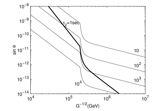
Figure 3 shows contours of the entropy increase due to sterile neutrino decay in the plane. We set the freeze–out temperature to , which maximizes ; this can be achieved by chosing the mass appropriately. The thick line indicates the BBN limit on the sterile neutrino lifetime, sec. Eq.(25) shows that for given neutrino mass, the released entropy will be maximal if is chosen such that reaches this upper limit.
The behavior of the contours in Fig. 3 is easy to understand from Eq.(25). In the relevant limit and keeping constant, we have for . The entropy ratio thus scales as for . Along the sec contour, the entropy release increases proportional to both for and for . Fig. 3 can be extended to even smaller , i.e. larger masses, so long as is smaller than the re–heat temperature after inflation, so that was in thermal equilibrium in the RD epoch. If at the same time is decreased so that sec remains constant, very large entropy dilution factors could be realized,
| (29) |
This result is only valid if the mixing–induced interactions of are not in thermal equilibrium for . Since these interactions are also responsible for decay, this assumption is satisfied whenever ; we saw in the discussion of Eq.(25) that this strong inequality is in any case a condition for significant entropy release from decay.
We finally note that for given the entropy released in decays is maximal if is so small that was ultra–relativistic at decoupling, since this maximizes . Again setting sec by appropriate choice of , this yields
| (30) |
6 Conclusion
In this paper we have developed an approximate analytic method for calculating the thermally–averaged annihilation cross section of semi–relativistically decoupling particles and for estimating their relic density. We have shown that this approximate solution can be smoothly matched to the well–known non–relativistic approximation at the point of intersection. We have argued that such relics cannot form the observed cosmological dark matter. However, we pointed out that the late decay of metastable semi–relativistically decoupling relics can be an efficient source of entropy production. As an example of this entropy production mechanism we discussed a scenario with a sterile neutrino, and illustrated to what extent entropy can be increased.
Acknowledgments
This work was partially supported by the Marie Curie Training Research Network “UniverseNet” under contract no. MRTN-CT-2006-035863, and by the European Network of Theoretical Astroparticle Physics ENTApP ILIAS/N6 under contract no. RII3-CT-2004-506222. The work of M.K. was also supported by the Marie Curie Training Research Network “HEPTools” under contract no. MRTN-CT-2006-035505.
Appendix A: Modified Bessel Functions
In this appendix, we summarize some properties of the modified Bessel function. Using an integral representation, the modified Bessel function of the second kind is defined by
| (31) |
In particular, the calculation of the relic abundance involves and ,
| (32) |
The lower order terms of the series expansion of and are given by
| (33) |
The asymptotic expansion of is given by
| (34) |
Appendix B: Validity of the Maxwell–Boltzmann Distribution
In the calculations of this paper we used the Maxwell–Boltzmann (MB) distribution also for particles that were semi–relativistic at decoupling; this assumption is e.g. implicit in Eq.(14). At first sight this seems quite dangerous. For example, at , i.e. , the MB result for overestimates the Fermi–Dirac distribution by about 7%, and underestimates the Bose–Einstein distribution by about 10%. Since annihilation always involves two particles, one might assume that the total error associated with the use of the MB distribution is about twice as large. In this Appendix we show that the MB distribution can indeed be used to compute the thermally averaged cross section and the decoupling temperature as long as . For smaller , one has to use the proper Fermi–Dirac or Bose–Einstein distribution only in the very last step, when calculating .
We begin by expanding the true distribution function,
| (35) |
where the upper (lower) sign is for fermionic (bosonic) particles. Note that the correction term in parentheses has exactly the same form as the “statistics factors” appearing in the collision term of the full Boltzmann equation [2]. For consistency these statistics factors therefore also have to be included. Up to first order in these correction factors, the temperature dependent terms in the integrand defining the collision term for processes then read for fermionic :
| (36) | |||||
here is independent of energy as long as is in kinetic equilibrium (through elastic scattering on SM particles); in that case we can equivalently write . In order to derive the full collision term, has to be multiplied with the squared matrix element and integrated over phase space [2].
In the usual treatment of WIMP decoupling, all the exponential terms in the square parentheses are neglected, so that the collision term becomes proportional to times the thermally averaged cross section defined in Eq.(14). Unfortunately the full correction term introduces additional dependence on the final state energies and . In order to keep the numerics manageable, we assume that they can be replaced by and , respectively. This is certainly true (by energy conservation) for the sum ; this has already been used in deriving Eq.(36). Note furthermore that we’ll need the collision term for temperatures , where , so that we can approximate . These approximations yield
| (37) |
where (3/2) for bosonic (fermionic) particles. In the following we will assume to be fermionic, which according to Eq.(37) should lead to larger deviations from the MB result.
Inserting this corrected collision term into the Boltzmann equation, and following the formalism of [7], finally yields a modified thermally averaged cross section times initial state velocity:
| (38) | |||||
with , and . This reduces to Eq.(14) if the expression in square parentheses is simply replaced by 1. In the following we assume that particles annihilate from an wave. wave annihilation would favor larger energies, where the correction terms in Eq.(38) are smaller. Note that we also have to use the expanded form (35) of the distribution function when calculating in Eq.(38); otherwise the solution of the Boltzmann equation will not yield , including the correction terms, at .
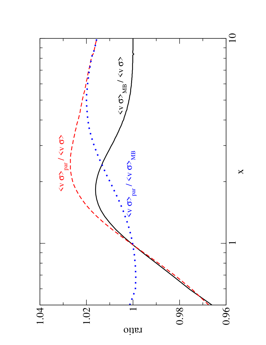
The size of the correction terms in Eq.(38) is illustrated by the solid (black) curve in Fig. 4. We see that the correction amounts to less than 2% for all . This is due to a strong cancellation between the corrections in the integrand of Eq.(38) and those in the overall factor . The dashed (red) curve shows that for the errors due to the use of the MB distribution and due to our simple parameterization (19) add up, leading to a total error of about 2.7% at most. The Fermi–Dirac corrections to the thermally averaged cross section begin to be significant for . However, here one enters the ultrarelativistic regime, where the final relic density is no longer sensitive to the decoupling temperature. We therefore expect the effect of using the MB distribution in Eq.(14) on the final prediction of the relic density to be quite small throughout.

This is illustrated in Fig. 5, where the relic density has been calculated using the simple assumption ; we have used the same parameters as in Fig. 2. The dashed (red) curve shows that using the MB distribution everywhere will overestimate the relic density for MeV, i.e. for . However, the black curve shows that this can easily be corrected by using the Fermi–Dirac distribution only in the final step, i.e. when calculating ; and can still been calculated using the MB distribution. This validates our treatment in the main text.
References
- [1] WMAP Collab., D. N. Spergel et al., Astrophys. J. Suppl. 148, 175 (2003), astro–ph/0302209; WMAP Collab., D. N. Spergel et al., Astrophys. J. Suppl. 170, 377 (2007), astro–ph/0603449; WMAP Collab., E. Komatsu et al., arXiv:0803.0547 [astro–ph].
- [2] E. W. Kolb and M. S. Turner, The Early Universe, Addison–Wesley (Redwood City, CA, 1990).
- [3] For reviews, see, e.g. G. Jungman, M. Kamionkowski and K. Griest, Phys. Rep. 267, 195 (1996); G. Bertone, D. Hooper and J. Silk, Phys. Rep. 405, 279 (2005), hep–ph/0404175.
- [4] R. Cowsik and J. McClelland, Phys. Rev. Lett. 29, 669 (1972).
- [5] R. J. Scherrer and M. S. Turner, Phys. Rev. D33, 1585 (1986), Erratum-ibid. D34, 3263 (1986).
- [6] K. Griest and D. Seckel, Phys. Rev. D43, 3191 (1991).
- [7] P. Gondolo and G. Gelmini, Nucl. Phys. B 360, 145 (1991).
- [8] P. J. Steinhardt and M. S. Turner, Phys. Lett. B 129, 51 (1983).
- [9] R. J. Scherrer and M. S. Turner, Phys. Rev. D 31, 681 (1985); G. Lazarides, R. K. Schaefer, D. Seckel and Q. Shafi, Nucl. Phys. B346, 193 (1990); J. E. Kim, Phys. Rev. Lett. 67, 3465 (1991).
- [10] S. Dodelson and L. M. Widrow, Phys. Rev. Lett. 72, 17 (1994), hep–ph/9303287; X. D. Shi and G. M. Fuller, Phys. Rev. Lett. 82, 2832 (1999), astro–ph/9810076]; A. D. Dolgov and S. H. Hansen, Astropart. Phys. 16, 339 (2002), hep–ph/0009083.
- [11] G. F. Giudice, E. W. Kolb and A. Riotto, Phys. Rev. D 64, 023508 (2001), hep-ph/0005123; G. B. Gelmini and P. Gondolo, Phys. Rev. D 74, 023510 (2006), hep-ph/0602230; G. Gelmini, P. Gondolo, A. Soldatenko and C. E. Yaguna, Phys. Rev. D 74, 083514 (2006), hep-ph/0605016.
- [12] M. Drees, H. Iminniyaz and M. Kakizaki, Phys. Rev. D 73, 123502 (2006), hep-ph/0603165.
- [13] B. W. Lee and S. Weinberg, Phys. Rev. Lett. 39, 165 (1977).
- [14] D.A. Dicus, E.W. Kolb and V.L. Teplitz, Phys. Rev. Lett. 39, 168 (1977), and Astrophys. J. 221, 327 (1978); M.I. Vysotsky, A.D. Dolgov and Ya.B. Zeldovich, Pisma Zh. Eksp. Teor. Fiz. 26, 200 (1977) [Sov. Phys. JETP Lett. 26, 188 (1977)]; D.A. Dicus, E.W. Kolb, V.L. Teplitz and R.V. Wagoner, Phys. Rev. D 17, 1529 (1978); E.W. Kolb and R.J. Scherrer, Phys. Rev. D 25, 1481 (1982); S. Sarkar and A.M. Cooper, Phys. Lett. 148B, 347 (1984).
- [15] C. Boehm, D. Hooper, J. Silk, M. Casse and J. Paul, Phys. Rev. Lett. 92, 101301 (2004), astro–ph/0309686; P. Fayet, Phys. Rev. D 70, 023514 (2004), hep-ph/0403226; N. Borodatchenkova, D. Choudhury and M. Drees, Phys. Rev. Lett. 96, 141802 (2006), hep–ph/0510147.
- [16] See e.g. the review of Big Bang Nucleosynthesis in the Particle Data Booklet, C. Amsler et al., Phys. Lett. B 667, 1 (2008).
- [17] J. McDonald, Phys. Rev. D 50,3637 (1994), hep–ph/0702143; C.P. Burgess, M. Pospelov and T. ter Veldhuis, Nucl. Phys. B 619, 709 (2001), hep–ph/0011335.
- [18] See e.g. the review on neutrino mixing in the Particle Data Booklet, C. Amsler et al., Phys. Lett. B 667, 1 (2008).
- [19] A. Boyarsky, J. Lesgourgues, O. Ruchayskiy and M. Viel, JCAP 0905, 012 (2009), arXiv:0812.0010 [astro–ph].
- [20] A recent analysis is K. Kohri, T. Moroi and A. Yotsuyanagi, Phys. Rev. D 73, 123511 (2006), hep-ph/0507245.
- [21] See e.g. J.R. Ellis, K.A. Olive, Y. Santoso and V.C. Spanos, Phys. Lett. B 565, 176 (2003), hep–ph/0303043.
- [22] For a review, see K. Enqvist and A. Mazumdar, Phys. Rep. 380, 99 (2003), hep–ph/0209244. Late Affleck–Dine baryogenesis has been discussed in E.D. Stewart, M. Kawasaki and T. Yanagida, Phys. Rev. D 54, 6032 (1996), hep-ph/9603324; M. Kawasaki and K. Nakayama, Phys. Rev. D 74, 123508 (2006), hep-ph/0608335.
- [23] M. Kawasaki, K. Kohri and N. Sugiyama, Phys. Rev. Lett. 82, 4168 (1999), astro–ph/9811437, and Phys. Rev. D62, 023506 (2000), astro–ph/0002127; S. Hannestad, Phys. Rev. D70, 043506 (2004), astro–ph/0403291; K. Ichikawa, M. Kawasaki and F. Takahashi, Phys. Rev. D72, 043522 (2005), astro–ph/0505395.