Purely Flavored Leptogenesis

D. Aristizabal Sierra^a, Luis Alfredo Muñoz^b, Enrico Nardi^a,b

^a INFN, Laboratori Nazionali di Frascati,C.P. 13, I00044 Frascati, Italy.

^b Instituto de Física, Universidad de Antioquia, A.A.1226, Medellín, Colombia.

We study a model for leptogenesis in which the total CP asymmetries in the decays and scatterings involving the $SU(2)$ singlet seesaw neutrinos $N_{\alpha}$ vanish ($\epsilon_{N_{\alpha}}=0$). Leptogenesis is possible due to non-vanishing CP violating lepton flavor asymmetries, realizing a situation in which the baryon asymmetry is due exclusively to flavor effects. We study the production of a net lepton asymmetry by solving the Boltzmann equations specific to this model, and we show that successful leptogenesis can be obtained at a scale as low as the TeV. We also discuss constraints on the model parameter space arising from current experimental upper limits on lepton flavor violating decays.

1 Introduction

Leptogenesis [1, 2] (for a comprehensive review see ref. [3]) is a theoretical mechanism that can explain the observed matter-antimatter asymmetry of the Universe. An initial lepton asymmetry, generated in the out-of-equilibrium decays of heavy singlet Majorana neutrinos, is partially converted in a baryon asymmetry by anomalous sphaleron interactions [4] that are standard model (SM) processes. Heavy Majorana singlet neutrinos are also a fundamental ingredient of the seesaw model [5], that provides an elegant explanation for the suppression of the neutrino masses with respect to all other SM mass scales. Leptogenesis can be quantitatively successful with a neutrino mass scale of the order of the atmospheric neutrino mass squared difference. This remarkable ‘coincidence’ links nicely the explanation of neutrino masses and of the baryon asymmetry within a single framework, and renders the idea that baryogenesis occurred through leptogenesis a very attractive one.

In the standard seesaw case, computations of the CP violating (CPV) asymmetries $\epsilon_{N_{\alpha}}$ in the decays of the $N_{\alpha}$ singlet neutrinos include loop diagrams in which Majorana states appear in the internal lines [6], and thus are lepton number violating quantities [7]. This is the reason why leptogenesis can proceed even when it is assumed that only one lepton flavor is relevant, as is the case at large temperatures ($T\ \hbox to0.0pt{\raise 3.0pt\hbox{$>$}\hss}{\lower 3.0pt\hbox{$\sim$}}\ 10^{12}\,$GeV). However, at temperatures below $\sim 10^{12}\,$GeV, lepton flavor dynamics plays an important role in leptogenesis, and cannot be neglected [8, 9] (See [10, 11] for earlier studies of flavor effects in leptogenesis, and [3, 12] for recent reviews). In particular, in ref. [9] it was pointed out that leptogenesis can occur even when $\epsilon_{N_{\alpha}}=0$, provided that the individual flavored CPV asymmetries $\epsilon_{N_{\alpha}\to L_{j}}$ (with $j=e,\mu,\tau$) are non vanishing.

Of course, $\epsilon_{N_{\alpha}}=\sum_{j}\epsilon_{N_{\alpha}\to L_{j}}=0$ means that total lepton number is not violated in $N_{\alpha}$ decays. The reason why leptogenesis can still occur even in this case can be understood by analogy with the generation of a baryon asymmetry $\Delta B=B-\bar{B}$ from a lepton asymmetry $\Delta L=L-\bar{L}$ that, as is well known, does not require any baryon number violating CP asymmetry. Baryon number, or more precisely $\Delta B+\Delta L$, is in fact violated in the plasma by fast sphaleron reactions, with the result that part of $\Delta L$ is converted in $\Delta B$ yielding a ratio $\Delta B/\Delta L=-28/51$.

Similarly, at $T\sim M_{N_{\alpha}}$ various interactions that are lepton and lepton flavor number violating occur in the plasma, like for example $\Phi\ell_{j}\leftrightarrow N_{\alpha}\leftrightarrow\bar{\Phi}\bar{\ell}_{k}$. Of course, these reactions must be at least slightly out-of-equilibrium, otherwise they would quickly drive the individual $\Delta L_{j}\to 0$. However, the important point here is that generically these (washout) reactions proceed with different rates for different lepton flavors, erasing more efficiently, say, $\Delta L_{\tau}$ than $\Delta L_{e,\mu}$. As a result, at $T\ll M_{N_{1}}$ ($N_{1}$ being the lightest heavy Majorana neutrino), once all washout processes are switched off, quite generically $\sum_{j}\Delta L_{j}=\Delta L\neq 0$ results. This scenario, in which leptogenesis can proceed solely because of flavor effects, is what we call Purely Flavored Leptogenesis (PFL). It is worth noticing that PFL realizes the Sakharov conditions [13] in a slightly different way that standard leptogenesis, since violation of lepton number occurs only in the washouts, while CP is violated only in the flavor charges, and the two conditions are thus disentangled.

Ref. [14] analyzed the issue of the interplay between the lepton number breaking scale and the breaking scale of a flavor symmetry (of the Froggatt-Nielsen type [15]). It was found that in the case when the flavor symmetry is still unbroken during the leptogenesis era, but the vectorlike messengers masses are larger than the Majorana neutrino mass, the total CP asymmetry vanishes and a PFL scenario arises. In this paper we show that the PFL model of ref. [14] can indeed succeed in producing the cosmological baryon asymmetry. Interestingly, in this model there is an upper limit on the leptogenesis temperature fixed by the requirement that leptogenesis must occur in the flavored regime ($T\ \hbox to0.0pt{\raise 3.0pt\hbox{$<$}\hss}{\lower 3.0pt\hbox{$\sim$}}\ 10^{12}\,$GeV) but, differently from the standard case, there is no lower limit and, as we will show, leptogenesis can be successful at a scale as low as the TeV.

The rest of the paper is organized as follows: in section 2 we recall the main features of the model, we give the expressions for the flavor CPV asymmetries and we discuss an important rescaling property of the CPV asymmetries that leaves unaffected the washout rates. In section 3 we write down the Boltzmann Equations (BE) for the model and we present the main results. In section 5 we study some relations between the flavor violating parameters of the model and the low energy limits on lepton flavor violating processes.

In our model washout and asymmetries in decays and scatterings occur at the same order in the couplings, and thus the derivation of the BE differs from the standard case in a non-trivial way. In appendix A we present a detailed derivation of the BE, that relies on the formalism introduced in ref. [16] to deal in a proper way with CPV asymmetries in scatterings. In appendix B we collect some definitions and useful formulae.

2 The Model

The model we consider here [14] is a simple extension of the SM containing a set of $SU(2)_{L}\times U(1)_{Y}$ fermion singlets, namely three right-handed neutrinos ($N_{\alpha}=N_{\alpha R}+N_{\alpha R}^{c}$) and three heavy vectorlike fields ($F_{a}=F_{aL}+F_{aR}$). In addition, we assume that at some high energy scale, taken to be of the order of the leptogenesis scale $M_{N_{1}}$, an exact $U(1)_{X}$ horizontal symmetry forbids direct couplings of the lepton $\ell_{i}$ and Higgs $\Phi$ doublets to the heavy Majorana neutrinos $N_{\alpha}$. At lower energies, $U(1)_{X}$ gets spontaneously broken by the vacuum expectation value $\sigma$ of a $SU(2)_{L}$ singlet scalar field $S$. Accordingly, the Yukawa interactions of the high energy Lagrangian read

$$-{\cal L}_{Y}=\frac{1}{2}\bar{N}_{\alpha}M_{N_{\alpha}}N_{\alpha}+\bar{F}_{a}M_{F_{a}}F_{a}+h_{ia}\bar{\ell}_{i}P_{R}F_{a}\Phi+\bar{N}_{\alpha}\left(\lambda_{\alpha a}+\lambda^{(5)}_{\alpha a}\gamma_{5}\right)F_{a}S+\mbox{h.c.}$$ (1)

We use Greek indices $\alpha,\beta\dots=1,2,3$ to label the heavy Majorana neutrinos, Latin indices $a,b\dots=1,2,3$ for the vectorlike messengers, and $i,j,k,\dots$ for the lepton flavors $e,\mu,\tau$. Following reference [14] we chose the simple $U(1)_{X}$ charge assignments $X(\ell_{L_{i}},F_{L_{a}},F_{R_{a}})=+1$, $X(S)=-1$ and $X(N_{\alpha},\Phi)=0$. This assignment is sufficient to enforce the absence of $\bar{N}\ell\Phi$ terms, but clearly it does not constitute an attempt to reproduce the fermion mass pattern, and accordingly we will also avoid assigning specific charges to the right-handed leptons and quark fields that have no relevance for our analysis. The important point is that it is likely that any flavor symmetry (of the Froggatt-Nielsen type) will forbid the the same tree-level couplings, and will reproduce an overall model structure similar to the one we are assuming here. Therefore we believe that our results, that are focused on a new realization of the leptogenesis mechanism, can hint to a general possibility that could well occur also in a complete model of flavor.

As it was discussed in [14], depending on the hierarchy between the relevant scales of the model ($M_{N_{1}},\,M_{F_{a}},\,\sigma$), quite different scenarios for leptogenesis can arise. PFL arises when the relevant scales satisfy the hierarchy $\sigma<M_{N_{1}}<M_{F_{a}}$ that is, when the flavor symmetry $U(1)_{X}$ is still unbroken during the leptogenesis era and at the same time the messengers $F_{a}$ are too heavy to be produced in $N_{1}$ decays and scatterings, and can be integrated away. As is explicitely shown by the last term in eq. (1), in general the vectorlike fields can couple to the heavy singlet neutrinos via scalar and pseudoscalar couplings, In ref. [14] it was assumed for simplicity a strong hierarchy $\lambda\gg\lambda^{(5)}$ which allowed us to neglect all the $\lambda^{(5)}$. However, in all the relevant quantities (scatterings, CP asymmetries, light neutrino masses) at leading order the scalar and pseudoscalar couplings always appear in the combination $\lambda+\lambda^{(5)}$, and thus such an assumption is not necessary. The replacement $\lambda\to\lambda+\lambda^{(5)}$ would suffice to include in the analysis the effects of both type of interactions.

2.1 Extended seesaw and light neutrino masses

Figure 1: Effective seesaw operator for the light neutrino masses

After $U(1)_{X}$ and electroweak symmetry breaking the Lagrangian eq. (1) generates masses for the light neutrinos through the effective mass operator depicted in figure 1. The resulting mass matrix reads [14]

$$-{\cal M}_{ij}=\left[h^{*}\frac{\sigma}{M_{F}}\lambda^{T}\frac{v^{2}}{M_{N}}\lambda\frac{\sigma}{M_{F}}h^{\dagger}\right]_{ij}=\left[\tilde{\lambda}^{T}\frac{v^{2}}{M_{N}}\tilde{\lambda}\right]_{ij}\,,$$ (2)

where we have introduced effective seesaw-like couplings defined as

$$\tilde{\lambda}_{\alpha i}=\left(\lambda\frac{\sigma}{M_{F}}h^{\dagger}\right)_{\alpha i}=\frac{\sigma}{M_{N_{1}}}\left(\lambda.r.h^{\dagger}\right)_{\alpha i}\,.$$ (3)

Note that, differently from standard seesaw, the neutrino mass matrix is of fourth order in the fundamental couplings ($h$ and $\lambda$) and includes an additional suppression factor of $(\sigma/M_{F})^{2}$.

2.2 $N_{1}$ decays and CPV asymmetries

Differently from standard leptogenesis in the present case, since $M_{F}>M_{N_{1}}$, two-body $N_{1}$ decays are kinematically forbidden. However, via off-shell exchange of the heavy $F_{a}$ fields, $N_{1}$ can decay to the three body final states $S\Phi l$ and $\bar{S}\bar{\Phi}\bar{l}$. The corresponding Feynman diagram is depicted in figure 2$(a)$. At leading order in $r_{a}=M_{N_{1}}/M_{F_{a}}$, the total decay width reads [14]

$$\Gamma_{N_{1}}\equiv\sum_{j}\Gamma(N_{1}\to S\Phi l_{j}+\bar{S}\bar{\Phi}\bar{l}_{j})=\frac{M_{N_{1}}}{192\pi^{3}}\left(\frac{M_{N_{1}}}{\sigma}\right)^{2}(\tilde{\lambda}\tilde{\lambda}^{\dagger})_{11}\,.$$ (4)

As usual, CPV asymmetries in $N_{1}$ decays arise from the interference between tree-level and one-loop amplitudes. As was noted in [14], in this model at one-loop there are no contributions from vertex corrections, and the only contribution to the CPV asymmetries comes from the self-energy diagram 2$(b)$. Summing over the leptons and vectorlike fields running in the loop, at leading order in $r_{a}$ the CPV asymmetry for $N_{1}$ decays into leptons of flavor $j$ can be written as

$$\epsilon_{1j}\equiv\epsilon_{N_{1}\to\ell_{j}}=\frac{3}{128\pi}\frac{\sum_{m}\mbox{Im}\left[\left(hr^{2}h^{\dagger}\right)_{mj}\tilde{\lambda}_{1m}\tilde{\lambda}^{*}_{1j}\right]}{\left(\tilde{\lambda}\tilde{\lambda}^{\dagger}\right)_{11}}\,.$$ (5)

Note that since the loop correction does not violate lepton number, the total CPV asymmetry that is obtained by summing over the flavor of the final state leptons vanishes [7], that is $\epsilon_{1}\equiv\sum_{j}\epsilon_{1j}=0$. This is the condition that defines PFL; namely there is no CPV and lepton number violating asymmetry, and the CPV lepton flavor asymmetries are the only seed of the Cosmological lepton and baryon asymmetries.

It is important to note that the effective couplings $\tilde{\lambda}$ defined in eq. (3) are invariant under the reparameterization

$$\lambda\to\lambda\cdot(rU)^{-1},\quad h^{\dagger}\to(Ur)\cdot h^{\dagger}\,,$$ (6)

where $U$ is an arbitrary $3\times 3$ non-singular matrix. Clearly the light neutrino mass matrix is invariant under this transformation. Moreover, also the flavor dependent washout processes, that correspond to tree level amplitudes that are determined, to a good approximation, by the effective $\tilde{\lambda}$ couplings, are left essentially unchanged. On the contrary, the flavor CPV asymmetries eq. (5), that are determined by loop amplitudes containing an additional factor of $hr^{2}h^{\dagger}$, get rescaled as $hr^{2}h^{\dagger}\to h(rUr)^{\dagger}(rUr)h^{\dagger}$. Clearly, this rescaling affects in the same way all the lepton flavors (as it should be to guarantee that the PFL conditions $\epsilon_{\alpha}\equiv\sum\epsilon_{\alpha j}=0$ are not spoiled), and thus for simplicity we will consider only rescaling by a global scalar factor $r.U=U.r=\kappa\,I$ (with $I$ the $3\times 3$ identity matrix) that, for our purposes, is completely equivalent to the more general transformation (6). Thus, while rescaling the Yukawa couplings through

$$\lambda\to\lambda\,\kappa^{-1},\quad h^{\dagger}\to\kappa\,h^{\dagger}\,,$$ (7)

does not affect neither low energy neutrino physics nor the washout processes, the CPV asymmetries get rescaled as:

$$\epsilon_{1j}\to\kappa^{2}\epsilon_{1j}\,.$$ (8)

By choosing $\kappa>1$, all the CPV asymmetries get enhanced as $\kappa^{2}$ and, being the Cosmological asymmetries generated through leptogenesis linear in the CPV asymmetries, the final result gets enhanced by the same factor. Therefore, for any given set of couplings, one can always find an appropriate rescaling such that the correct amount of Cosmological lepton asymmetry is generated. In practice, the rescaling factors $\kappa$ cannot be arbitrarily large: first, they should respect the condition that all the fundamental Yukawa couplings remain in the perturbative regime; second, as will be discussed in section 5, the size of the $h$ couplings (and thus also of the rescaling parameter $\kappa$) is also constrained by experimental limits on lepton flavor violating decays.

Figure 2: Feynman diagrams responsible for the CPV asymmetry.

3 Boltzmann Equations

In this section we compute the lepton asymmetry by solving the appropriate BE. In general, to consistently derive the evolution equation of the lepton asymmetry all the possible processes at a given order in the couplings have to be included. In the present case $1\leftrightarrow 3$ decays and inverse decays, and $2\leftrightarrow 2$ $s$, $t$ and $u$ channel scatterings all occur at the same order in the couplings and must be included altogether in the BE. The Feynman diagrams for these processes are shown in Figure 3. In addition, the CPV asymmetries of some higher order multiparticle reactions involving the exchange of one off-shell $N_{1}$, also contribute to the source term of the asymmetries at the same order in the couplings than the CPV asymmetries of decays and $2\leftrightarrow 2$ scatterings. More precisely, for a proper derivation of the BE it is essential that the CPV asymmetries of the off-shell $3\leftrightarrow 3$ and $2\leftrightarrow 4$ scattering processes depicted in figures 7, and 8 in appendix A, are also taken into account. In order to do this, we follow Ref. [16] and we split the BE for the evolution of the density asymmetry of the flavor $\ell_{i}$ as:

$$\dot{Y}_{\Delta L_{i}}=(\dot{Y}_{\Delta L_{i}})_{1\leftrightarrow 3}+(\dot{Y}_{\Delta L_{i}})_{2\leftrightarrow 2}+(\dot{Y}_{\Delta L_{i}})_{3\leftrightarrow 3}^{\mbox{\tiny{sub}}}+(\dot{Y}_{\Delta L_{i}})_{2\leftrightarrow 4}^{\mbox{\tiny{sub}}}\,,$$ (9)

where $Y_{\Delta L_{i}}=(n_{\ell_{i}}-n_{\bar{\ell}_{i}})/s$ with $n_{\ell_{i}}$ ($n_{\bar{\ell}_{i}}$) the number density of $\ell_{i}$ (anti)leptons, and $s$ the entropy density. The time derivative is defined as $\dot{Y}\equiv s\,H\,z\,dY/dz$ where $z=M_{N_{1}}/T$ and $H$ is the Hubble parameter. The first term on the r.h.s. of eq. (9) represents the contribution of three body decays and inverse decays, the second term that of $2\leftrightarrow 2$ scatterings, the third term is defined in terms of the off-shell (pole subtracted) $3\leftrightarrow 3$ multiparticle density rates $\gamma_{3\leftrightarrow 3}^{\mbox{\tiny{sub}}}=\gamma_{3\leftrightarrow 3}-\gamma_{3\leftrightarrow 3}^{\mbox{\tiny{on-shell}}}$, and similarly for the fourth term. The BE for $Y_{\Delta_{\ell_{i}}}$ is derived by taking into account in full the first two terms on the r.h.s., while for the remaining two terms only the corresponding CP asymmetry is important, since non-resonant contributions to the washouts from multiparticle processes are always negligible.

As regards the equation for the evolution of the heavy neutrino density $Y_{N_{1}}$, only the diagrams in fig. 3, that are of leading order in the couplings, are important. We refer to appendix A for a detailed derivation of the equations. The final result reads

$$\dot{Y}_{N_{1}} =-\left(y_{N_{1}}-1\right)\gamma_{\text{tot}}$$ (10)

$$\dot{Y}_{\Delta L_{i}} =\left(y_{N_{1}}-1\right)\epsilon_{i}\gamma_{\text{tot}}-\Delta y_{i}\left[\gamma_{i}+\left(y_{N_{1}}-1\right)\gamma^{N_{1}\bar{\ell}_{i}}_{S\Phi}\right]\,,$$ (11)

where in the last term of the second equation we have used the compact notation for the reaction densities $\gamma^{N_{1}\bar{\ell}_{i}}_{S\Phi}=\gamma(N_{1}\bar{\ell}_{i}\to{S\Phi})$. $\gamma_{i}$ and $\gamma_{\text{tot}}$ are defined as

$$\gamma_{i} = \gamma^{N_{1}}_{S\ell_{i}\Phi}+\gamma^{N_{1}\bar{S}}_{\Phi\ell_{i}}+\gamma^{N_{1}\bar{\Phi}}_{S\ell_{i}}+\gamma_{S\Phi}^{N_{1}\bar{\ell}_{i}}$$ (12)

$$\gamma_{\text{tot}} = \sum_{i=e,\mu,\tau}\gamma_{i}+\bar{\gamma}_{i},$$ (13)

where in the second equation $\bar{\gamma}_{i}$ represents the sum of the CP conjugates of the processes summed in $\gamma_{i}$.

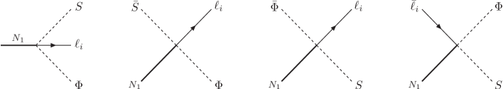
Figure 3: Feynman diagrams for $1\leftrightarrow 3$ and $2\leftrightarrow 2$ $s$, $t$ and $u$ channel processes after integrating out the heavy vectorlike fields $F_{a}$.

Since in this model $N_{1}$ decays are of the same order in the couplings than scatterings (that is ${\cal O}(\tilde{\lambda}^{2})$), the appropriate condition that defines the strong washout regime in the case at hand reads:

$$\left.\frac{\gamma_{\text{tot}}}{z\,H\,s}\right|_{z\sim 1}>1\,\qquad{\rm(strong\ washout)},$$ (14)

and conversely $\gamma_{\text{tot}}/(z\,H\,s)|_{z\sim 1}<1$ defines the weak washout regime. Note that this is different from standard leptogenesis, where at $z\sim 1$ two body decays generally dominate over scatterings, and e.g. the condition for the strong washout regime can be approximated as $\gamma_{\text{tot}}/(z\,H\,s)|_{z\sim 1}\sim\Gamma_{N_{1}}/H|_{z\sim 1}>1$.

4 Results

In this section we discuss a typical example of successful leptogenesis at the scale of a few TeV. The example presented is a general one. No particular choice of the parameters has been performed, except for the fact that the low energy neutrino data are reproduced within errors, and that the choice yields an interesting washout dynamics well suited to illustrate how PFL works. The numerical value of the final lepton asymmetry ($Y_{\Delta L}\sim-5.4\times 10^{-10}$) is about a factor of 3 larger than what is indicated by measurements of the Cosmic baryon asymmetry. This is however irrelevant since, as was discussed in section 2., it would be sufficient a minor rescaling of the couplings (or a slight change in the CPV phases) to obtain the precise experimental result. In the numerical analysis we have neglected the dynamics of the heavier singlet neutrinos since the $N_{\alpha}$ masses are sufficiently hierarchical to ensure that $N_{2,3}$ related washouts do not interfere with $N_{1}$ dynamics. Moreover, in the (strong washout) fully flavored regime (that is effective as long as $T<10^{9}\,$GeV) the $N_{2,3}$ CPV asymmetries do not contribute to the final lepton number asymmetry [18].

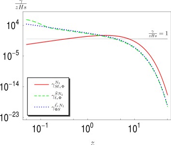
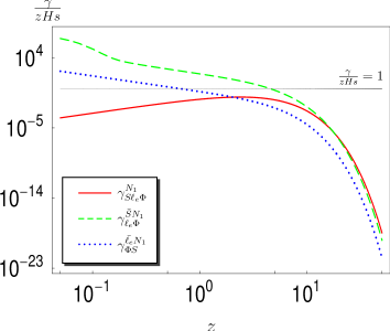
Figure 4: Reaction densities normalized to $zHs$ for $N_{1}\to S\ell\Phi$ decays (red solid lines), $s$-channel $\bar{S}N_{1}\leftrightarrow\ell\Phi$ scatterings (green dashed lines), and $t,u$-channel scatterings in the point-like approximation (blue dotted lines). Left panel: $\tau$ flavor. Right panel: electron flavor.

In figure 4 we show the behavior of the various reaction densities for decays and scatterings, normalized to $sHz$, as a function of $z=M_{N_{1}}/T$. The results correspond to a mass of the lightest singlet neutrino fixed to $M_{N_{1}}=2.5\,\text{TeV}$, the heavier neutrino masses are $M_{N_{2}}=10\,$TeV and $M_{N_{3}}=15\,$TeV, and the relevant mass ratios $r_{a}=M_{N_{1}}/M_{F_{a}}$ for the messenger fields are $r_{1,2,3}=0.1,0.01,0.001$ (the effects of the lightest $F$ resonances can be seen in the $s$-channel rates in both panels in fig. 4). The fundamental Yukawa couplings $h$ and $\lambda$ are chosen to satisfy the requirement that the seesaw formula eq. (2) reproduces within $2\,\sigma$ the low energy data on the neutrino mass squared differences and mixing angles [19]. Typically, when this requirement is fulfilled, one also ends up with a dynamics for all the lepton flavors in the strong washout regime. This is shown in the left panel in fig. 5 where we present the total rates for the three flavors.

The left panel in fig. 4 refers to the decay and scattering rates involving the $\tau$-flavor that, in our example, is the flavor more strongly coupled to $N_{1}$, and that thus suffers the strongest washout. It is worth noticing that, due to the fact that in this model scatterings are not suppressed by additional coupling constants with respect to the decays, the decay rate starts dominating the washouts only at $z\ \hbox to0.0pt{\raise 3.0pt\hbox{$>$}\hss}{\lower 3.0pt\hbox{$\sim$}}\ 1$. The right panel in fig. 4 depicts the reaction rates for the electron flavor, that is the more weakly coupled, and for which the strong washout condition eq. (14) is essentially ensured by sizeable $s$-channel scatterings. Scatterings and decay rates for the $\mu$-flavor are not shown, but they are in between the ones of the previous two flavors.

The total reaction densities that determine the washout rates for the different flavors are shown in the first panel in figure 5. The evolution of these rates with $z$ should be confronted with the evolution of (the absolute value of) the asymmetry densities for each flavor, depicted in the second panel on the right. Since, as already stressed several times, PFL is defined by the condition that the sum of the flavor CPV asymmetry vanishes ($\sum_{j}\epsilon_{1j}=0$), it is the hierarchy between these washout rates that in the end is the responsible for generating a net lepton number asymmetry. In the case at hand, the absolute values of the flavor CPV asymmetries satisfy the condition $|\epsilon_{\mu}|<|\epsilon_{e}|<|\epsilon_{\tau}|$, as can be inferred directly by the fact that at $z<0.1$, when the effects of the washouts are still negligible, the asymmetry densities satisfy this hierarchy. Moreover, since $\epsilon_{\mu,e}<0$ while $\epsilon_{\tau}>0$, initially the total lepton number asymmetry, that is dominated by $Y_{\Delta L_{\tau}}$, is positive. As washout effects become important, the $\tau$-related reactions (blue dotted line in the left panel) start erasing $Y_{\Delta L_{\tau}}$ more efficiently than what happens for the other two flavors, and thus the initial positive asymmetry is driven towards zero, and eventually changes sign around $z=0.2$. This change of sign corresponds to the steep valley in the absolute value $|Y_{\Delta L}|$ that is drawn in the figure with a black solid line. Note that when all flavors are in the strong washout regime, as in the present case, the condition for the occurrence of this ‘sign inversions’ is simply given by ${\rm max_{j\in e,\mu}}\left(|\epsilon_{j}|/|\tilde{\lambda}_{1j}|^{2}\right)\ \hbox to0.0pt{\raise 3.0pt\hbox{$>$}\hss}{\lower 3.0pt\hbox{$\sim$}}\ \epsilon_{\tau}/|\tilde{\lambda}_{1\tau}|^{2}$. From this point onwards, the asymmetry remains negative, and since the electron flavor is the one that suffers the weakest washout, $Y_{\Delta L_{e}}$ ends up dominating all the other density asymmetries. In fact, as can be seen from the right panel in fig. 5, it is $Y_{\Delta L_{e}}$ that determines to a large extent the final value of the lepton asymmetry $Y_{\Delta L}=-5.4\times 10^{-10}$.

A few comments are in order regarding the role played by the $F_{a}$ fields. Even if $M_{N_{1}}\ll M_{F_{a}}$, at large temperatures $z\gg 1$ the tail of the thermal distributions of the $N_{1},\,S$ and $\Phi$ particles allows the on-shell production of the lightest $F$ states. A possible asymmetry generated in the decays of the $F$ fields can be ignored for two reasons: first because due to the rather large $h$ and $\lambda$ couplings $F$ decays occur to a good approximation in thermal equilibrium, ensuring that no sizeable asymmetry can be generated, and second because the strong washout dynamics that characterizes $N_{1}$ leptogenesis at lower temperatures is in any case insensitive to changes in the initial conditions.

In conclusion, it is clear from the results of this section that the model encounters no difficulties to allow for the possibility of generating the Cosmic baryon asymmetry at a scale of a few TeVs. Moreover, our analysis provides a concrete example of PFL, and shows that the condition $\epsilon_{1}\neq 0$ is by no means required for successful leptogenesis.

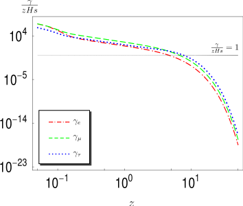
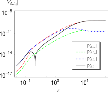
Figure 5: Left panel: the total washout rates for each lepton flavor normalized to $zHs$ as a function of $z$. Right panel: the evolution of the absolute value of the flavored density asymmetries and of the lepton number asymmetry (black solid line). The flavor CPV asymmetries are $\epsilon_{1e}=-4.7\times 10^{-4}$, $\epsilon_{1\mu}=-1.9\times 10^{-4}$ and $\epsilon_{1\tau}=6.6\times 10^{-4}$. The final values of the asymmetry densities (at $z\gg 1$) are $Y_{\Delta L_{e}}=-7.1\times 10^{-10}$, $Y_{\Delta L_{\mu}}=-0.3\times 10^{-10}$, $Y_{\Delta L_{\tau}}=2.0\times 10^{-10}$.

5 Lepton Flavor Violating Decays

We have seen that a particular feature of this model is that the rescaling of the couplings eq. (7) can enhance the CPV asymmetry by a factor $\kappa^{2}$ (see eq. (8)) without affecting neither the low energy neutrino physics nor the washout rates. In practice, it is this decoupling of the CPV asymmetries from the washouts that renders possible lowering the leptogenesis scale down to the TeV. It is then natural to ask how large the rescaling factor $\kappa$ can be, or in other words how large the $h$ couplings can become, without incurring in the violation of some phenomenological bound. To this aim, in this section we will derive upper bounds on the Yukawa couplings $h_{ia}$ from the non-observation of Lepton Flavor Violating (LFV) decays. The set of Yukawa interactions involving the heavy vectorlike fields $F_{a}$, the $SU(2)$ Higgs scalar $\Phi$ and lepton doublets $\ell_{i}$, can induce lepton flavor violating radiative decays $\ell_{i}\to\ell_{j}\gamma$. Here we will concentrate on $\mu\to e\gamma$ that is the most constrained process. Note that, with respect to the radiative decays, lepton flavor violating decays like $\ell^{\prime}\to 3\ell$ are more suppressed since they are induced by box diagrams rather then by penguin-type diagrams. Therefore we will not consider them.

The partial decay width for the lepton flavor violating decay $\ell_{i}\to\ell_{j}\gamma$ reads

$$\Gamma(\ell_{i}\to\ell_{j}\gamma)=\frac{\alpha}{1024\pi^{4}}\frac{m_{i}^{5}}{M_{W}^{4}}\left|\sum_{a=1}^{3}h_{ia}^{*}h_{ja}F(M_{W}^{2}/M_{F_{a}}^{2})\right|^{2}\,.$$ (15)

Here $M_{W}$ is the $W^{\pm}$ $SU(2)$ gauge boson mass which enter the loop through its longitudinal component $\Phi^{\pm}$ and $m_{i}$ is the mass of the decaying lepton (the mass of the final state lepton $m_{j}$ has been neglected). $F(x)$ is a loop function given by

$$F(x)=\frac{x}{12(1-x)^{4}}\left(2+3x-6x^{2}+x^{3}+6x\log x\right)$$ (16)

and for $x\to 0$, $F(x)\to x/6$. Since $M_{F_{a}}\gg M_{W}$, $F(M_{W}^{2}/M_{F_{a}}^{2})$ strongly suppresses the LFV radiative decays and thus, in general, the Yukawa couplings $h_{ia}$ will not be strongly constrained by the current experimental upper limits. In fact, as is shown in fig. 6, for $M_{F}>$ a few TeVs and Yukawa couplings $\ \hbox to0.0pt{\raise 3.0pt\hbox{$<$}\hss}{\lower 3.0pt\hbox{$\sim$}}\ .5$, the radiative LFV decay rates always remain far below the present limits. Only for $h\ \hbox to0.0pt{\raise 3.0pt\hbox{$>$}\hss}{\lower 3.0pt\hbox{$\sim$}}\ 2$ (that is close to the perturbative limit represented by the hatched region in fig. 6) and $M_{F_{1}}\sim 25\,$TeV (that was our choice in the numerical example) the $\mu\to e\gamma$ decay rate becomes comparable to the present sensitivity, and is well within the reach of future experiments [20]. Thus we can safely conclude that present limits on LFV decays do not place any serious constraint on the viability of TeV scale leptogenesis within the PFL model discussed in this paper.

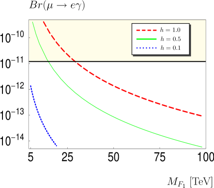
Figure 6: $Br(\mu\to e\gamma)$ as a function of the mass of the lightest vectorlike field $F_{1}$. No hierarchy for the $h$ couplings and a mild hierarchy for the $F$ masses ($M_{F_{3}}=1.3\cdot M_{F_{2}}=2\cdot M_{F_{1}}$) has been assumed. The region above the horizontal line is excluded by current experimental limits. The hatched region corresponds to non-perturbative couplings $h>\sqrt{4\pi}$.

6 Conclusions

Variations of the standard leptogenesis scenario can arise from the presence of additional (flavor) symmetries broken around or below the scale at which lepton number is effectively broken. Quite generically, the resulting scenarios can yield new qualitative and quantitative changes on the way leptogenesis is realized. Here we have considered a model in which an Abelian $U(1)_{X}$ flavor symmetry, still unbroken during the leptogenesis era, is added to the SM gauge symmetry group. We have also assumed that the messengers fields responsible for the effective mass operators of the light particles are heavier that the lightest Majorana neutrino $N_{1}$ and thus, during leptogenesis, cannot be produced. The model has the remarkable feature that the total CPV asymmetry in $N_{1}$ decays vanishes, while the lepton flavor asymmetries are generically nonvanishing, and thus it constitutes an explicit realization of the scenario that we have called purely flavored leptogenesis.

By using the BE specific for this model, we have studied the evolution of the asymmetry densities for the different lepton flavors as the temperature changes, and we have found that successful leptogenesis can occur at a scale as low as a few TeVs. This possibility is due to the fact that the size of the flavored CPV asymmetries is decoupled from the strength of the washouts and from low energy neutrino physics. This allows to rescale the CPV asymmetries up to rather large values, leaving unaffected the washout rates as well as the light neutrino masses and mixings. Our model shows that if new unbroken symmetries are present at a scale below the leptogenesis scale, this could have a very interesting and even surprising impact on the way leptogenesis is realized.

7 Acknowledgments

LAM would like to thank short term training fellowships from the EU HELEN program and hospitality from the INFN-LNF Theory Group in Frascati (Rome). The work of EN is supported in part by Colciencias under contract 1115-333-18739.

Appendix A Boltzmann Equations

Following mainly ref. [16], we start by introducing a set of compact notations. We normalize particle densities to the equilibrium densities, $y_{a}\equiv Y_{a}/Y_{a}^{\text{eq}}$ where $Y_{a}=n_{a}/s$ with $n_{a}$ the particle number density and $s$ the entropy density, and we define the time derivative as $\dot{Y}=sHz\,dY/dz$. Reaction densities are denoted by $\gamma_{B}^{A}$ where $A$ and $B$ are respectively the initial and final states of the specific decay or scattering process. As in eq. (9), we divide he BE for the evolution of the density asymmetry of the flavor $\ell_{i}$ ${Y}_{\Delta L_{i}}\equiv Y_{\ell_{i}}-Y_{\bar{\ell}_{i}}$ into different contributions

$$\dot{Y}_{\Delta L_{i}}=(\dot{Y}_{\Delta L_{i}})_{1\leftrightarrow 3}+(\dot{Y}_{\Delta L_{i}})_{2\leftrightarrow 2}+(\dot{Y}_{\Delta L_{i}})_{3\leftrightarrow 3}^{\mbox{\tiny{sub}}}+(\dot{Y}_{\Delta L_{i}})_{2\leftrightarrow 4}^{\mbox{\tiny{sub}}}\,,$$ (17)

and we derive the explicit form of the different contributions in the following sections.

A.1 $1\leftrightarrow 3$ and $2\leftrightarrow 2$ processes

The contributions $(\dot{Y}_{\Delta L_{i}})_{1\leftrightarrow 3}$ and $(\dot{Y}_{\Delta L_{i}})_{2\leftrightarrow 2}$ in eq. (17) arise from the $1\leftrightarrow 3$ and $2\leftrightarrow 2$ reactions depicted in figure 3, that are all of ${\cal O}(\lambda^{2}h^{2})$. Using CPT invariance ($\gamma^{A}_{B}=\gamma^{\bar{B}}_{\bar{A}}$) and after linearizing in the CPV asymmetries and in the asymmetry densities $\Delta y_{a}\equiv y_{a}-y_{\bar{a}}$ they can be written as:

$$(\dot{Y}_{\Delta L_{i}})_{N_{1}\leftrightarrow\Phi S\ell_{i}} =(y_{N_{1}}+1)\Delta\gamma^{N_{1}}_{S\ell_{i}\Phi}-(\Delta y_{S}+\Delta y_{\Phi}+\Delta y_{\ell_{i}})\gamma^{N_{1}}_{S\ell_{i}\Phi},$$ (18)

$$(\dot{Y}_{\Delta L_{i}})_{N\bar{S}\leftrightarrow\Phi\ell_{i}} =(y_{N_{1}}+1)\Delta\gamma^{N_{1}\bar{S}}_{\Phi\ell_{i}}-(y_{N_{1}}\Delta y_{S}+\Delta y_{\Phi}+\Delta y_{\ell_{i}})\gamma^{N_{1}\bar{S}}_{\Phi\ell_{i}},$$ (19)

$$(\dot{Y}_{\Delta L_{i}})_{N\bar{\Phi}\leftrightarrow S\ell_{i}} =(y_{N_{1}}+1)\Delta\gamma^{N_{1}\bar{\Phi}}_{S\ell_{i}}-(\Delta y_{S}+y_{N_{1}}\Delta y_{\Phi}+\Delta y_{\ell_{i}})\gamma^{N_{1}\bar{\Phi}}_{S\ell_{i}},$$ (20)

$$(\dot{Y}_{\Delta L_{i}})_{N\bar{\ell}_{i}\leftrightarrow\Phi S} =(y_{N_{1}}+1)\Delta\gamma_{S\Phi}^{N_{1}\bar{\ell_{i}}}-(\Delta y_{S}+\Delta y_{\Phi}+y_{N_{1}}\Delta y_{\ell_{i}})\gamma_{S\Phi}^{N_{1}\bar{\ell_{i}}}\,,$$ (21)

where $(\dot{Y}_{\Delta\ell_{i}})_{N\bar{S}\leftrightarrow\Phi\ell_{i}}$, $(\dot{Y}_{\Delta L_{i}})_{N\bar{\Phi}\leftrightarrow S\ell_{i}}$ and $(\dot{Y}_{\Delta L_{i}})_{N\bar{\ell}_{i}\leftrightarrow\Phi S}$ are the $s$, $t$ and $u$ channel contributions to the $2\leftrightarrow 2$ scattering term $(\dot{Y}_{\Delta L_{i}})_{2\leftrightarrow 2}$. For completeness, in these equations as well as in the following we keep trace of the density asymmetries $\Delta y_{\Phi}$ and $\Delta y_{S}$ of the Higgs and of the $S$-scalar. This is needed if one wishes to take into account spectator processes [21]. The related effects (that can be as large as 40%  [21]) depend, however, on the specific interactions of $S$ with other particles (quarks) and are thus model dependent, and have been neglected in the present analysis. After summing up eqs. (18-21) we obtain

$$(\dot{Y}_{\Delta L_{i}})_{1\leftrightarrow 3}+(\dot{Y}_{\Delta L_{i}})_{2\leftrightarrow 2} =(y_{N_{1}}+1)(\Delta\gamma^{N_{1}}_{S\ell_{i}\Phi}+\Delta\gamma^{N_{1}\bar{S}}_{\Phi\ell_{i}}+\Delta\gamma^{N_{1}\bar{\Phi}}_{S\ell_{i}}+\Delta\gamma_{S\Phi}^{N_{1}\bar{\ell}_{i}})$$

$$-\Delta y_{\ell_{i}}(\gamma^{N_{1}}_{S\ell_{i}\Phi}+\gamma^{N_{1}\bar{s}}_{\Phi\ell_{i}}+\gamma^{N_{1}\bar{\Phi}}_{s\ell_{i}}+y_{N_{1}}\gamma_{S\Phi}^{N_{1}\bar{\ell}_{i}})$$

$$-\Delta y_{\Phi}(\gamma^{N_{1}}_{S\ell_{i}\Phi}+\gamma^{N_{1}\bar{S}}_{\Phi\ell_{i}}+y_{N_{1}}\gamma^{N_{1}\bar{\Phi}}_{S\ell_{i}}+\gamma_{S\Phi}^{N_{1}\bar{\ell}_{i}})$$

$$-\Delta y_{S}(\gamma^{N_{1}}_{S\ell_{i}\Phi}+y_{N_{1}}\gamma^{N_{1}\bar{S}}_{\Phi\ell_{i}}+\gamma^{N_{1}\bar{\Phi}}_{S\ell_{i}}+\gamma_{S\Phi}^{N_{1}\bar{\ell}_{i}})\,.$$ (22)

As is usual when only lowest order processes are included in the BE, the factor $(y_{N_{1}}+1)$ signals an incorrect thermodynamical behavior (generation of an asymmetry in thermal equilibrium). In order to get the correct result we need to include in the BE also the CPV asymmetries of higher order processes, like the $3\leftrightarrow 3$ and $2\leftrightarrow 4$ scatterings in which one $N_{1}$ is exchanged as a virtual state in the internal lines. This is carried out in the following two sections.

A.2 $3\leftrightarrow 3$ processes

Multiparticle tree level processes in which one $N_{1}$ is exchanged in one internal line can be divided into on-shell and off-shell parts. For the on-shell parts, when the $N_{1}$ line in the amplitude is cut, we obtain either the $1\leftrightarrow 3$ or the $2\leftrightarrow 2$ diagrams in fig. 3 which were already accounted for in eq. (A.1). We then have to consider only the off-shell contributions, denoted as $\gamma^{\prime}$, where the superscript is a reminder that the given reaction has the on-shell piece subtracted out. The contribution of these off-shell processes to the washouts is negligible; however, the contribution of their CPV asymmetries cannot be neglected. Figure 7 shows the set of Feynman diagrams for $3\leftrightarrow 3$ scattering processes yielding $|\Delta L_{i}|=2$. They are of two types: $\ell_{i}\leftrightarrow\bar{\ell}_{i}$ and $\ell_{i}\ell_{i}\leftrightarrow 0$. We do not show the analogous $|\Delta L_{i}|=1$ diagrams, since they can have either one $\bar{\ell}_{j}$ or one $\ell_{j}$ ($j\neq i$) attached to one external leg, and for this reason their number is rather large.

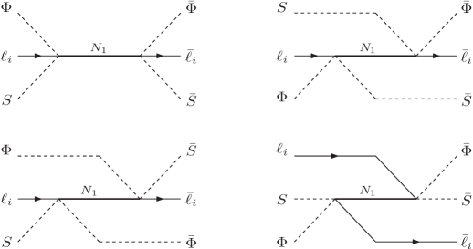
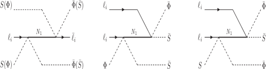
Figure 7: Feynman diagrams for $3\leftrightarrow 3$ scattering processes yielding $|\Delta L_{i}|=2$. $\Phi\ell_{i}S\leftrightarrow\bar{\Phi}\bar{\ell}_{i}\bar{S}$ (first four diagrams); $S\ell_{i}S\leftrightarrow\bar{\Phi}\bar{\ell}_{i}\bar{\Phi}$ (and $\Phi\ell_{i}\Phi\leftrightarrow\bar{S}\bar{\ell}_{i}\bar{S}$) (fifth diagram); $\ell_{i}\ell_{i}\Phi\leftrightarrow\bar{\Phi}\bar{S}\bar{S}$ and $\ell_{i}\ell_{i}S\leftrightarrow\bar{\Phi}\bar{\Phi}\bar{S}$ (last two diagrams).

Since the CPV asymmetries of the full processes are of higher order in the couplings, at ${\cal O}(\lambda^{2}h^{4})$ the asymmetries of the off-shell parts are equal in magnitude and opposite in sign to the CPV asymmetries of their on-shell parts. In turn, the latter’s are directly related to the CPV asymmetry in $N_{1}$ decays and scatterings. Denoting the on shell parts of the rates as $\gamma^{(\text{on})}$, we then have:

$$\Delta\gamma^{\prime A}_{B}=-\Delta\gamma^{(\text{on})\,A}_{B}\,.$$ (23)

The on-shell pieces of the $3\leftrightarrow 3$ reactions for $|\Delta L_{i}|=2$ processes can be written as

$$\gamma^{(\text{on})\,\Phi\ell_{i}S}_{\bar{\Phi}\bar{\ell}_{i}\bar{S}} =\gamma^{\Phi\ell_{i}S}_{N_{1}}P^{N_{1}}_{\bar{\Phi}\bar{\ell}_{i}\bar{S}}+\gamma^{\Phi\ell_{i}}_{\bar{S}N_{1}}P^{SN_{1}}_{\bar{\Phi}\bar{\ell}_{i}}+\gamma^{S\ell_{i}}_{\bar{\Phi}N_{1}}P^{\Phi N_{1}}_{\bar{S}\bar{\ell}_{i}}+\gamma^{S\Phi}_{\bar{\ell}_{i}N_{1}}P^{\ell_{i}N_{1}}_{\bar{S}\bar{\Phi}},$$ (24)

$$\gamma^{(\text{on})\,S\ell_{i}S}_{\bar{\Phi}\bar{\ell}_{i}\bar{\Phi}} =\gamma^{S\ell_{i}}_{\bar{\Phi}N_{1}}P^{SN_{1}}_{\bar{\ell}_{i}\bar{\Phi}},$$ (25)

$$\gamma^{(\text{on})\,\Phi\ell_{i}\Phi}_{\bar{S}\bar{\ell}_{i}\bar{S}} =\gamma^{\Phi\ell_{i}}_{\bar{S}N_{1}}P^{\Phi N_{1}}_{\bar{\ell}_{i}\bar{S}},$$ (26)

$$\gamma^{(\text{on})\,\Phi SS}_{\bar{\ell}_{i}\bar{\ell}_{i}\bar{\Phi}} =\gamma^{\Phi S}_{\bar{\ell}_{i}N_{1}}P^{SN_{1}}_{\bar{\ell}_{i}\bar{\Phi}},$$ (27)

$$\gamma^{(\text{on})\,\Phi S\Phi}_{\bar{\ell}_{i}\bar{\ell}_{i}\bar{S}} =\gamma^{\Phi S}_{\bar{\ell}_{i}N_{1}}P^{\Phi N_{1}}_{\bar{\ell}_{i}\bar{S}}\,.$$ (28)

The $P^{A}_{B}$ represents the (decay or scattering) probability for the transition $A\to B$, and were introduced in [16] to generalize the zero temperature branching ratios to the finite temperature case, when the $N_{1}$’s have a finite probability to scatter inelastically with particles in the plasma before decaying. We have for example:

$$P^{N_{1}}_{\bar{\Phi}\bar{\ell}_{i}\bar{S}}=\frac{\gamma^{N_{1}}_{\bar{\Phi}\bar{\ell}_{i}\bar{S}}}{\gamma_{\text{tot}}},\qquad P^{SN_{1}}_{\bar{\Phi}\bar{\ell}_{i}}=\frac{\gamma^{SN_{1}}_{\bar{\Phi}\bar{\ell}_{i}}}{\gamma_{\text{tot}}},\qquad{\rm etc.},$$ (29)

where

$$\gamma_{\text{tot}}=\sum_{i}\left(\gamma_{S\Phi\ell_{i}}^{N_{1}}+\gamma_{\bar{S}\bar{\Phi}\bar{\ell}_{i}}^{N_{1}}+\gamma_{\ell_{i}\Phi}^{\bar{S}N_{1}}+\gamma_{\bar{\ell}_{i}\bar{\Phi}}^{SN_{1}}+\gamma_{\ell_{i}S}^{\bar{\Phi}N_{1}}+\gamma_{\bar{\ell}_{i}\bar{S}}^{\Phi N_{1}}+\gamma_{\Phi S}^{\ell_{i}N_{1}}+\gamma_{\bar{\Phi}\bar{S}}^{\bar{\ell}_{i}N_{1}}\right)\,.$$ (30)

Using the set of equations (24-28) together with the corresponding CP conjugate equations, including the contributions from $|\Delta L_{i}|=1$ processes, and defining ${\cal P}^{a}_{b}\equiv P^{a}_{b}+P^{\bar{a}}_{\bar{b}}$, the different contributions to $(\dot{Y}_{\Delta\ell_{i}})_{3\leftrightarrow 3}^{\mbox{\tiny{sub}}}$ can be written as:

$$(\dot{Y}_{\Delta L_{i}})_{\Phi\ell_{i}S\leftrightarrow\bar{\Phi}\bar{\ell_{j}}\bar{S}} =-\Delta\gamma^{N_{1}}_{S\Phi\ell_{i}}\sum_{j}{\cal P}^{N_{1}}_{S\Phi\ell_{j}}-\Delta\gamma^{N_{1}\bar{\Phi}}_{S\ell_{i}}\sum_{j}{\cal P}^{N_{1}\bar{\Phi}}_{S\ell_{j}}$$

$$\quad-\Delta\gamma^{N_{1}\bar{S}}_{\Phi\ell_{i}}\sum_{j}{\cal P}^{N_{1}\bar{S}}_{\Phi\ell_{j}}-\Delta\gamma^{\bar{\Phi}\bar{S}}_{N_{1}\ell_{i}}\sum_{j}{\cal P}^{N_{1}\bar{\ell}_{j}}_{\Phi S}\,,$$

$$(\dot{Y}_{\Delta\ell_{i}})_{\Phi\ell_{i}S\leftrightarrow\Phi\ell_{j}S} =-\Delta\gamma^{N_{1}}_{S\Phi\ell_{i}}\sum_{j}{\cal P}^{N_{1}}_{S\Phi\ell_{j}}\,,$$

$$(\dot{Y}_{\Delta\ell_{i}})_{\Phi\ell_{i}\bar{S}\leftrightarrow\Phi\ell_{j}\bar{S}} =-\Delta\gamma^{N_{1}\bar{S}}_{\Phi\ell_{i}}\sum_{j}{\cal P}^{N_{1}\bar{S}}_{\Phi\ell_{j}}\,,$$

$$(\dot{Y}_{\Delta\ell_{i}})_{\bar{\Phi}\ell_{i}S\leftrightarrow\bar{\Phi}\ell_{j}S} =-\Delta\gamma^{N_{1}\bar{\Phi}}_{S\ell_{i}}\sum_{j}{\cal P}^{N_{1}\bar{\Phi}}_{S\ell_{j}}\,,$$

$$(\dot{Y}_{\Delta\ell_{i}})_{\bar{\Phi}\ell_{i}\bar{S}\leftrightarrow\bar{\Phi}\ell_{j}\bar{S}} =-\Delta\gamma^{\bar{\Phi}\bar{S}}_{N_{1}\ell_{i}}\sum_{j}{\cal P}^{N_{1}\bar{\ell}_{j}}_{\Phi S}\,,$$

$$(\dot{Y}_{\Delta L_{i}})_{S\ell_{i}S\leftrightarrow\bar{\Phi}\bar{\ell}_{j}\bar{\Phi}} =-\Delta\gamma^{N_{1}\bar{\Phi}}_{S\ell_{i}}\sum_{j}{\cal P}^{N_{1}\bar{S}}_{\Phi\ell_{j}}\,,$$

$$(\dot{Y}_{\Delta L_{i}})_{\Phi\ell_{i}\Phi\leftrightarrow\bar{S}\bar{\ell}_{j}\bar{S}} =-\Delta\gamma^{N_{1}\bar{S}}_{\Phi\ell_{i}}\sum_{j}{\cal P}^{N_{1}\bar{\Phi}}_{S\ell_{j}}\,,$$

$$(\dot{Y}_{\Delta L_{i}})_{\ell_{i}\ell_{j}\Phi\leftrightarrow\bar{S}\bar{\Phi}\bar{S}} =-\Delta\gamma^{N_{1}\bar{S}}_{\Phi\ell_{i}}\sum_{j}{\cal P}^{N_{1}\bar{\ell}_{j}}_{\Phi S}-\Delta\gamma^{\bar{\Phi}\bar{S}}_{N_{1}\ell_{i}}\sum_{j}{\cal P}^{N_{1}\bar{S}}_{\Phi\ell_{j}}\,,$$

$$(\dot{Y}_{\Delta L_{i}})_{\ell_{i}\ell_{j}S\leftrightarrow\bar{\Phi}\bar{S}\bar{\Phi}} =-\Delta\gamma^{N_{1}\bar{\Phi}}_{S\ell_{i}}\sum_{j}{\cal P}^{N_{1}\bar{\ell}_{j}}_{\Phi S}-\Delta\gamma^{\bar{\Phi}\bar{S}}_{N_{1}\ell_{i}}\sum_{j}{\cal P}^{N_{1}\bar{\Phi}}_{S\ell_{j}}\,,$$

$$(\dot{Y}_{\Delta L_{i}})_{S\ell_{i}\bar{S}\leftrightarrow\Phi\ell_{j}\bar{\Phi}} =-\Delta\gamma^{N_{1}\bar{\Phi}}_{S\ell_{i}}\sum_{j}{\cal P}^{N_{1}\bar{S}}_{\Phi\ell_{j}}-\Delta\gamma^{N_{1}\bar{S}}_{\Phi\ell_{i}}\sum_{j}{\cal P}^{N_{1}\bar{\Phi}}_{S\ell_{j}}\,,$$

$$(\dot{Y}_{\Delta L_{i}})_{\ell_{i}\bar{\ell_{j}}\Phi\leftrightarrow S\Phi\bar{S}} =-\Delta\gamma^{N_{1}\bar{S}}_{\Phi\ell_{i}}\sum_{j}{\cal P}^{N_{1}\bar{\ell}_{j}}_{\Phi S}-\Delta\gamma^{\bar{\Phi}\bar{S}}_{N_{1}\ell_{i}}\sum_{j}{\cal P}^{N_{1}\bar{S}}_{\Phi\ell_{j}}\,,$$

$$(\dot{Y}_{\Delta L_{i}})_{\ell_{i}\bar{\ell_{j}}S\leftrightarrow\Phi S\bar{\Phi}} =-\Delta\gamma^{N_{1}\bar{\Phi}}_{S\ell_{i}}\sum_{j}{\cal P}^{N_{1}\bar{\ell}_{j}}_{\Phi S}-\Delta\gamma^{\bar{\Phi}\bar{S}}_{N_{1}\ell_{i}}\sum_{j}{\cal P}^{N_{1}\bar{\Phi}}_{S\ell_{j}},$$ (31)

where in the l.h.s., of these equations, whenever the $\ell_{i}\leftrightarrow\ell_{j}$ transition is involved, it is left understood that $i\neq j$. To write the above relations, we have first completed the sums over flavor. For example for the second equation in (A.2):

$$(\dot{Y}_{\Delta\ell_{i}})_{\Phi\ell_{i}S\leftrightarrow\Phi\ell_{j}S} =-\Delta\gamma^{N_{1}}_{S\Phi\ell_{i}}\sum_{j\neq i}{\cal P}^{N_{1}}_{S\Phi\ell_{j}}+{\cal P}^{N_{1}}_{S\Phi\ell_{i}}\sum_{j\neq i}\Delta\gamma^{N_{1}}_{S\Phi\ell_{j}}$$

$$=-\Delta\gamma^{N_{1}}_{S\Phi\ell_{i}}\sum_{j}{\cal P}^{N_{1}}_{S\Phi\ell_{j}}+{\cal P}^{N_{1}}_{S\Phi\ell_{i}}\sum_{j}\Delta\gamma^{N_{1}}_{S\Phi\ell_{j}}\,.$$ (32)

We have then used the specific relations valid for PFL (equivalent to $\sum_{j}\epsilon_{j}=0$)

$$\sum_{j}\Delta\gamma^{N_{1}}_{S\Phi\ell_{j}}=\sum_{j}\Delta\gamma^{N_{1}\bar{S}}_{\Phi\ell_{j}}=\sum_{j}\Delta\gamma^{N_{1}\bar{\Phi}}_{S\ell_{j}}=\sum_{j}\Delta\gamma^{\bar{\Phi}\bar{S}}_{N_{1}\ell_{j}}=0.$$ (33)

Thus, the last term in the second line of eq. (A.2) vanishes, and the expression for $(\dot{Y}_{\Delta\ell_{i}})_{\Phi\ell_{i}S\leftrightarrow\Phi\ell_{j}S}$ given in (A.2) is obtained.

A.3 $2\leftrightarrow 4$ processes

The inclusion of $2\leftrightarrow 4$ processes proceeds along similar lines than for $3\leftrightarrow 3$ processes. As is shown by the diagrams in figure 8, there are three types of $|\Delta L_{i}|=2$ contributions to the evolution equation for $Y_{\Delta L_{i}}$. The on-shell pieces of these contributions can be written as:

$$\gamma^{(\text{on})\,\ell_{i}S}_{\bar{\Phi}\bar{S}\bar{\ell}_{i}\bar{\Phi}}=P^{\ell_{i}S}_{\bar{\Phi}N_{1}}\gamma^{N_{1}}_{\bar{S}\bar{\ell}_{i}\bar{\Phi}},\qquad\gamma^{(\text{on})\,\ell_{i}\Phi}_{\bar{S}\bar{S}\bar{\ell}_{i}\bar{\Phi}}=P^{\ell_{i}\Phi}_{\bar{S}N_{1}}\gamma^{N_{1}}_{\bar{S}\bar{\ell}_{i}\bar{\Phi}},\qquad\gamma^{(\text{on})\,\Phi S}_{\bar{\ell}_{i}\bar{S}\bar{\ell}_{i}\bar{\Phi}}=P^{\Phi S}_{\bar{\ell}_{i}N_{1}}\gamma^{N_{1}}_{\bar{S}\bar{\ell}_{i}\bar{\Phi}}\,.$$ (34)

By using again eq. (23) to relate the on-shell parts to the relevant off-shell pieces, including the CP conjugate relations and including also the $2\leftrightarrow 4$ processes with $|\Delta L_{i}|=1$, we obtain the following contributions:

$$(\dot{Y}_{\Delta L_{i}})_{\Phi\ell_{i}S\Phi\leftrightarrow\bar{S}\bar{\ell}_{j}} =-\Delta\gamma^{N_{1}\bar{\Phi}}_{S\ell_{i}}\sum_{j}{\cal P}^{N_{1}}_{S\Phi\ell_{j}}-\Delta\gamma^{N_{1}}_{S\Phi\ell_{i}}\sum_{j}{\cal P}^{N_{1}\bar{\Phi}}_{S\ell_{j}}$$

$$(\dot{Y}_{\Delta L_{i}})_{\Phi\ell_{i}SS\leftrightarrow\bar{\Phi}\bar{\ell}_{j}} =-\Delta\gamma^{N_{1}\bar{S}}_{\Phi\ell_{i}}\sum_{j}{\cal P}^{N_{1}}_{S\Phi\ell_{j}}-\Delta\gamma^{N_{1}}_{S\Phi\ell_{i}}\sum_{j}{\cal P}^{N_{1}\bar{S}}_{\Phi\ell_{j}}$$

$$(\dot{Y}_{\Delta L_{i}})_{\Phi\ell_{i}S\ell_{j}\leftrightarrow\bar{S}\bar{\Phi}} =-\Delta\gamma^{\bar{\Phi}\bar{S}}_{N_{1}\ell_{i}}\sum_{j}{\cal P}^{N_{1}}_{S\Phi\ell_{j}}-\Delta\gamma^{N_{1}}_{S\Phi\ell_{i}}\sum_{j}{\cal P}^{N_{1}\bar{\ell}_{j}}_{\Phi S}$$

$$(\dot{Y}_{\Delta L_{i}})_{\Phi\ell_{i}S\bar{\Phi}\leftrightarrow S\ell_{j}} =-\Delta\gamma^{N_{1}}_{S\Phi\ell_{i}}\sum_{j}{\cal P}^{N_{1}\bar{\Phi}}_{S\ell_{j}}-\Delta\gamma^{N_{1}\bar{\Phi}}_{S\ell_{i}}\sum_{j}{\cal P}^{N_{1}}_{S\Phi\ell_{j}}$$

$$(\dot{Y}_{\Delta L_{i}})_{\Phi\ell_{i}S\bar{S}\leftrightarrow\Phi\ell_{j}} =-\Delta\gamma^{N_{1}}_{S\Phi\ell_{i}}\sum_{j}{\cal P}^{N_{1}\bar{S}}_{\Phi\ell_{j}}-\Delta\gamma^{N_{1}\bar{S}}_{\Phi\ell_{i}}\sum_{j}{\cal P}^{N_{1}}_{S\Phi\ell_{j}}$$

$$(\dot{Y}_{\Delta L_{i}})_{\Phi\ell_{i}S\bar{\ell}_{j}\leftrightarrow S\Phi} =-\Delta\gamma^{N_{1}}_{S\Phi\ell_{i}}\sum_{j}{\cal P}^{N_{1}\bar{\ell}_{j}}_{\Phi S}-\Delta\gamma^{\bar{\Phi}\bar{S}}_{N_{1}\ell_{i}}\sum_{j}{\cal P}^{N_{1}}_{S\Phi\ell_{j}}.$$ (35)

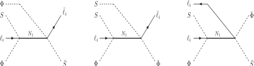
Figure 8: Feynman diagrams for the $2\leftrightarrow 4$ with $|\Delta L_{i}|=2$ reactions $S\ell_{i}\leftrightarrow\bar{\Phi}\bar{S}\bar{\ell}_{i}\bar{\Phi}$, $\ell_{i}\Phi\leftrightarrow\bar{S}\bar{S}\bar{\ell}_{i}\bar{\Phi}$ and $\Phi S\leftrightarrow\bar{\ell}_{i}\bar{S}\bar{\ell}_{i}\bar{\Phi}$.

From the sets of equations (A.1), (A.2) and (A.3), and using $\sum_{j}({\cal P}^{N_{1}}_{\Phi\ell_{j}S}+{\cal P}^{N_{1}\bar{S}}_{\ell_{j}\Phi}+{\cal P}^{N_{1}\bar{\Phi}}_{\ell_{j}S}+{\cal P}^{N_{1}\bar{\ell}_{j}}_{S\Phi})=1$, we finally obtain the BE for the evolution of $Y_{\Delta L_{i}}$:

$$\dot{Y}_{\Delta L_{i}} =(y_{N_{1}}-1)(\Delta\gamma^{N_{1}}_{S\ell_{i}\Phi}+\Delta\gamma^{N_{1}\bar{S}}_{\Phi\ell_{i}}+\Delta\gamma^{N_{1}\bar{\Phi}}_{S\ell_{i}}+\Delta\gamma_{S\Phi}^{N_{1}\bar{\ell}_{i}})$$ (36)

$$-\Delta y_{\ell_{i}}(\gamma^{N_{1}}_{S\ell_{i}\Phi}+\gamma^{N_{1}\bar{S}}_{\Phi\ell_{i}}+\gamma^{N_{1}\bar{\Phi}}_{S\ell_{i}}+y_{N_{1}}\gamma_{S\Phi}^{N_{1}\bar{\ell}_{i}})$$

$$-\Delta y_{\Phi}(\gamma^{N_{1}}_{S\ell_{i}\Phi}+\gamma^{N_{1}\bar{S}}_{\Phi\ell_{i}}+y_{N_{1}}\gamma^{N_{1}\bar{\Phi}}_{S\ell_{i}}+\gamma_{S\Phi}^{N_{1}\bar{\ell}_{i}})$$

$$-\Delta y_{S}(\gamma^{N_{1}}_{S\ell_{i}\Phi}+y_{N_{1}}\gamma^{N_{1}\bar{S}}_{\Phi\ell_{i}}+\gamma^{N_{1}\bar{\Phi}}_{S\ell_{i}}+\gamma_{S\Phi}^{N_{1}\bar{\ell}_{i}})\,.$$

where the term $(y_{N_{1}}-1)$ in the r.h.s. shows that the correct thermodynamical behavior is recovered.

Finally, using the approximate equalities between the scatterings and the decay asymmetries  [16]

$$\frac{\Delta\gamma^{N_{1}}_{\ell_{i}\Phi S}}{\gamma^{N_{1}}_{\ell_{i}\Phi S}}\simeq\frac{\Delta\gamma^{N_{1}\bar{\Phi}}_{\ell_{i}S}}{\gamma^{N_{1}\bar{\Phi}}_{\ell_{i}S}}\simeq\frac{\Delta\gamma^{N_{1}\bar{S}}_{\ell_{i}\Phi}}{\gamma^{N_{1}\bar{S}}_{\ell_{i}\Phi}}\simeq\frac{\Delta\gamma^{N_{1}\bar{\ell}_{i}}_{\Phi S}}{\gamma^{N_{1}\bar{\ell}_{i}}_{\Phi S}}\,,$$ (37)

the source term in equation (36) can be rewritten as

$$\left(\dot{Y}_{\Delta L_{i}}\right)_{\rm source}=(y_{N_{1}}-1)\frac{\Delta\gamma^{N_{1}}_{\ell_{i}\Phi S}}{\gamma^{N_{1}}_{\ell_{i}\Phi S}}\>\gamma_{i}\,,$$ (38)

where $\gamma_{i}=\gamma^{N_{1}}_{\ell_{i}\Phi S}+\gamma^{N_{1}\bar{\Phi}}_{\ell_{i}S}+\gamma^{N_{1}\bar{S}}_{\ell_{i}\Phi}+\gamma^{N_{1}\bar{\ell}_{i}}_{\Phi S}$. By using the relation

$$\frac{\gamma^{N_{1}}_{\ell_{i}\Phi S}}{\sum_{j}(\gamma^{N_{1}}_{\ell_{j}\Phi S}+\gamma^{N_{1}}_{\bar{\ell}_{i}\bar{\Phi}\bar{S}})}=\frac{\gamma_{i}}{\sum_{j}(\gamma_{j}+\bar{\gamma}_{j})}\,,$$ (39)

and recalling that the flavored CPV asymmetries are given by

$$\epsilon_{i}=\frac{\Delta\gamma^{N_{1}}_{\ell_{i}\Phi S}}{\sum_{j}(\gamma^{N_{1}}_{\ell_{j}\Phi S}+\gamma^{N_{1}}_{\bar{\ell}_{j}\bar{\Phi}\bar{S}})}$$ (40)

the evolution equation in (38) can be recast as

$$\dot{Y}_{\Delta L_{i}}= \epsilon_{i}\left(y_{N_{1}}-1\right)\gamma_{\text{tot}}-\Delta y_{i}\left[\gamma_{i}+\left(y_{N_{1}}-1\right)\gamma^{N_{1}\bar{\ell}_{i}}_{S\Phi}\right]$$

$$-\Delta y_{\Phi}\left[\gamma_{i}+\left(y_{N_{1}}-1\right)\gamma^{N_{1}\bar{\Phi}}_{S\ell_{i}}\right]-\Delta y_{S}\left[\gamma_{i}+\left(y_{N_{1}}-1\right)\gamma^{N_{1}\bar{S}}_{\Phi\ell_{i}}\right]\,,$$ (41)

where $\gamma_{\text{tot}}$ is given in eq. (30). Neglecting the terms in the second line proportional to $\Delta y_{\Phi}$ and $\Delta y_{S}$ amounts to neglect ${\cal O}(1)$ effects [21], and still yields a quite reasonable approximation. Finally, the evolution equation for the heavy Majorana neutrino can be simply written as:

$$\dot{Y}_{N_{1}}=-(y_{N_{1}}-1)\,\gamma_{\text{tot}}\,.$$ (42)

Appendix B Decay and Scatterings

The thermally averaged reaction density for $N_{1}\leftrightarrow\ell_{i}\Phi S$ is given by [2, 17]

$$\gamma^{N_{1}}_{\ell_{i}\Phi S}=N_{N_{1}}^{\text{eq}}\,\frac{K_{1}(z)}{K_{2}(z)}\,\Gamma^{N_{1}}_{\ell_{\Phi}S}\,,$$ (43)

where $N_{N_{1}}^{\text{eq}}$ is the equilibrium number density for $N_{1}$, $K_{1,2}(z)$ are Bessel functions (see appendix B in ref. [3]) and $\Gamma^{N_{1}}_{\ell_{\Phi}S}$ is the decay width given in (4). The thermally averaged $2\to 2$ reaction densities are given by

$$\gamma_{2\to 2}=\frac{M^{4}_{N_{1}}}{512\pi^{5}z}\int^{\infty}_{1}dx\sqrt{x}K_{1}\left(z\sqrt{x}\right)\hat{\sigma}\left(x\right)\,.$$ (44)

Here $\hat{\sigma}(x)$ is the dimensionless reduced cross section

$$\hat{\sigma}(x)=\sum_{a}r^{2}_{a}h^{*}_{ia}h_{ia}\lambda^{*}_{1a}\lambda_{1a}F^{a}(x)+2\sum_{a<b}r_{a}r_{b}\,\mathbb{R}\text{e}[h^{*}_{ia}h_{ib}\lambda^{*}_{1a}\lambda_{1b}G^{a,b}(x)].$$ (45)

The explicit form of the kinematical functions $F^{a}(x)$ and $G^{a,b}(x)$ depends on the specific $s$, $t$ or $u$ channel processes. In practice, for the $t$ and $u$ channels it is always a good approximation to use point-like interactions obtained by integrating out the heavy vectorlike fields. In this approximation, $\gamma^{N_{1}\bar{\Phi}}_{S\ell_{i}}=\gamma^{N_{1}\bar{\ell}_{i}}_{\Phi S}=\gamma^{t,u}_{2\to 2}$ where

$$\gamma_{2\to 2}^{t,u}=\frac{M^{4}_{N_{1}}}{1024\pi^{5}z}\left[\sum_{a}r^{2}_{a}h^{*}_{ia}h_{ia}\lambda^{*}_{1a}\lambda_{1a}+2\sum_{a<b}r_{a}r_{b}\,\mathbb{R}\text{e}(h^{*}_{ia}h_{ib}\lambda^{*}_{1a}\lambda_{1b})\right]\,f(z),$$ (46)

with

$$f(z)=\int_{1}^{\infty}\,dx\,\frac{x^{2}-1}{\sqrt{x}}\,K_{1}(z\sqrt{x})\,.$$ (47)

For $s$-channel scatterings ($N_{1}\bar{S}\leftrightarrow\ell_{i}\Phi$) the pointlike approximation is not sufficiently accurate, expecially at high temperatures $T>M_{N_{1}}$, and the complete expression for the kinematical functions has to be used. We define

$$G^{a,b}_{s}(x)=\frac{x-1}{H^{a,b}_{s,1}}\times[(1-x)\,H^{a,b}_{s,2}+(1+x)\,H^{a,b}_{s,3}]\,,$$ (48)

with

$$H^{a,b}_{s,1}(x) =2x(1-r_{a}^{2}x-2ir_{a}\eta_{a})(1-r_{b}^{2}x+2ir_{b}\eta_{b}),$$ (49)

$$H^{a,b}_{s,2}(x) =2r_{a}r_{b}+r_{a}+r_{b}+ir_{a}r_{b}(\eta_{a}-\eta_{b})+r_{a}r_{b}(x-1),$$ (50)

$$H^{a,b}_{s,3}(x) =r_{a}r_{b}+r_{a}+r_{b}+ir_{a}r_{b}(\eta_{a}-\eta_{b})+(1+ir_{a}\eta_{a})(1-ir_{b}\eta_{b})\,,$$ (51)

and

$$F^{a}_{s}(x)=G^{a,a}_{s}(x)\,.$$ (52)

The dimensionless parameter $\eta_{a}$ introduced in the equations above corresponds to the total decay widths of the messenger fields $F_{a}$ normalized to the $N_{1}$ neutrino mass:

$$\eta_{a}=\frac{\Gamma_{a}}{M_{N_{1}}}=\frac{1}{8\pi r_{a}}\left[(1-r^{2}_{a})(1+r_{a})^{2}\lambda^{*}_{1a}\lambda_{1a}+\frac{1}{2}\sum_{i}h^{*}_{ia}h_{ia}\right]\,.$$ (53)

References

- [1] M. Fukugita and T. Yanagida, Phys. Lett. B 174, 45 (1986).
- [2] M. A. Luty, Phys. Rev. D 45, 455 (1992).
- [3] S. Davidson, E. Nardi and Y. Nir, Phys. Rept. 466, 105 (2008) [arXiv:0802.2962 [hep-ph]].
- [4] V. A. Kuzmin, V. A. Rubakov and M. E. Shaposhnikov, Phys. Lett. B 155, 36 (1985).
- [5] P. Minkowski, Phys. Lett. B 67 421 (1977); T. Yanagida, in Proc. of Workshop on Unified Theory and Baryon number in the Universe, eds. O. Sawada and A. Sugamoto, KEK, Tsukuba, (1979) p.95; M. Gell-Mann, P. Ramond and R. Slansky, in Supergravity, eds P. van Niewenhuizen and D. Z. Freedman (North Holland, Amsterdam 1980) p.315; P. Ramond, Sanibel talk, retroprinted as hep-ph/9809459; S. L. Glashow, in Quarks and Leptons, Cargèse lectures, eds M. Lévy, (Plenum, 1980, New York) p. 707; R. N. Mohapatra and G. Senjanović, Phys. Rev. Lett. 44, 912 (1980).
- [6] L. Covi, E. Roulet and F. Vissani, Phys. Lett. B 384, 169 (1996) [arXiv:hep-ph/9605319].
- [7] E. W. Kolb and S. Wolfram, Nucl. Phys. B 172, 224 (1980) [Erratum-ibid. B 195, 542 (1982)].
- [8] A. Abada, S. Davidson, F. X. Josse-Michaux, M. Losada and A. Riotto, JCAP 0604 (2006) 004 [arXiv:hep-ph/0601083]; A. Abada, S. Davidson, A. Ibarra, F. X. Josse-Michaux, M. Losada and A. Riotto, JHEP 0609 (2006) 010 arXiv:hep-ph/0605281.
- [9] E. Nardi, Y. Nir, E. Roulet and J. Racker, JHEP 0601 (2006) 164 [arXiv:hep-ph/0601084].
- [10] R. Barbieri, P. Creminelli, A. Strumia and N. Tetradis, Nucl. Phys. B 575, 61 (2000) (for the updated version of this paper see [arXiv:hep-ph/9911315]).
- [11] T. Endoh, T. Morozumi and Z. h. Xiong, Prog. Theor. Phys. 111, 123 (2004) [arXiv:hep-ph/0308276]; T. Fujihara, S. Kaneko, S. Kang, D. Kimura, T. Morozumi and M. Tanimoto, Phys. Rev. D 72, 016006 (2005) [arXiv:hep-ph/0505076].
- [12] A. Strumia, arXiv:hep-ph/0608347; E. Nardi, arXiv:hep-ph/0702033; Y. Nir, arXiv:hep-ph/0702199; M. C. Chen, arXiv:hep-ph/0703087; E. Nardi, arXiv:0706.0487 [hep-ph].
- [13] A. D. Sakharov, Pisma Zh. Eksp. Teor. Fiz. 5 (1967) 32 [JETP Lett. 5 (1967 SOPUA,34,392-393.1991 UFNAA,161,61-64.1991) 24].
- [14] D. Aristizabal Sierra, M. Losada and E. Nardi, Phys. Lett. B 659, 328 (2008) [arXiv:0705.1489 [hep-ph]]; D. Aristizabal Sierra, Luis Alfredo Muñoz and Enrico Nardi, arXiv:0904.3052 [hep-ph].
-
[15]
C. D. Froggatt and H. B. Nielsen,
Nucl. Phys. B 147, 277 (1979).
- [16] E. Nardi, J. Racker and E. Roulet, JHEP 0709, 090 (2007) [arXiv:0707.0378 [hep-ph]].
- [17] G. F. Giudice, A. Notari, M. Raidal, A. Riotto and A. Strumia, Nucl. Phys. B 685, 89 (2004) [arXiv:hep-ph/0310123].
- [18] G. Engelhard, Y. Grossman, E. Nardi and Y. Nir, Phys. Rev. Lett. 99, 081802 (2007) [arXiv:hep-ph/0612187].
- [19] T. Schwetz, M. Tortola and J. W. F. Valle, New J. Phys. 10, 113011 (2008) [arXiv:0808.2016 [hep-ph]].
- [20] ‘MEG collaboration home page: http://meg.web.psi.ch/index.html.
- [21] E. Nardi, Y. Nir, J. Racker and E. Roulet, JHEP 0601, 068 (2006) [arXiv:hep-ph/0512052].