Quadrilateral-Octagon Coordinates for
Almost Normal Surfaces

Abstract

Normal and almost normal surfaces are essential tools for algorithmic 3-manifold topology, but to use them requires exponentially slow enumeration algorithms in a high-dimensional vector space. The quadrilateral coordinates of Tollefson alleviate this problem considerably for normal surfaces, by reducing the dimension of this vector space from $7n$ to $3n$ (where $n$ is the complexity of the underlying triangulation). Here we develop an analogous theory for octagonal almost normal surfaces, using quadrilateral and octagon coordinates to reduce this dimension from $10n$ to $6n$. As an application, we show that quadrilateral-octagon coordinates can be used exclusively in the streamlined 3-sphere recognition algorithm of Jaco, Rubinstein and Thompson, reducing experimental running times by factors of thousands. We also introduce joint coordinates, a system with only $3n$ dimensions for octagonal almost normal surfaces that has appealing geometric properties.

AMS Classification 57N10 (57Q35)

Keywords  Normal surfaces, almost normal surfaces, quadrilateral-octagon coordinates, joint coordinates, Q-theory, 3-sphere recognition

1 Introduction

The theory of normal surfaces, introduced by Kneser [17] and developed by Haken [8, 9], is central to algorithmic 3-manifold topology. In essence, normal surface theory allows us to search for “interesting” embedded surfaces within a 3-manifold triangulation $\mathcal{T}$ by enumerating the vertices of a polytope in a high-dimensional vector space. Normal surfaces are defined by their intersections with the tetrahedra of $\mathcal{T}$, which must be collections of disjoint triangles and/or quadrilaterals, collectively referred to as normal discs.

In the early 1990s, Rubinstein introduced the concept of an almost normal surface, for use with problems such as 3-sphere recognition and finding Heegaard splittings [21]. Almost normal surfaces are essentially normal surfaces with a single unusual intersection piece, which may be either an octagon or a tube. Thompson subsequently refined the 3-sphere recognition algorithm to remove any need for tubes [23], and since then almost normal surfaces have appeared in algorithms such as determining Heegaard genus [18], recognising small Seifert fibred spaces [22], and finding bridge surfaces in knot complements [27].

In this paper we focus on octagonal almost normal surfaces; that is, almost normal surfaces in which the unusual intersection piece is an octagon, not a tube. The reason for this restriction is that octagonal almost normal surfaces are both tractable and useful, and have important applications beyond 3-manifold topology. In detail:

• For practical computation, octagonal almost normal surfaces are significantly easier to deal with than general almost normal surfaces. In particular, the translation between surfaces and high-dimensional vectors becomes much simpler, and the enumeration of these vectors is less fraught with complications.

• As shown by Thompson [23], octagonal almost normal surfaces are sufficient for running the 3-sphere recognition algorithm.

• Following on from the previous point, an efficient 3-sphere recognition algorithm is important for computation in 4-manifold topology. For example, answering even the basic question “is $\mathcal{T}$ a 4-manifold triangulation?” requires us to run the 3-sphere recognition algorithm over a neighbourhood of each vertex of $\mathcal{T}$. Therefore, improving the efficiency of 3-sphere recognition is an important step towards a general efficient computational framework for working with 4-manifold triangulations.

As suggested above, our focus here is on the efficiency of working with almost normal surfaces. The fundamental problem that we face is that the underlying polytope vertex enumeration can grow exponentially slowly in the number of tetrahedra. This means that in practice normal surface algorithms cannot be run on large triangulations. Moreover, this exponential growth is not the fault of the algorithms, but an unavoidable feature of the problems that they try to solve. For illustrations of this, see [7] which describes cases in which the underlying vertex enumeration problem has exponentially many solutions, or see the proof by Agol et al. that computing 3-manifold knot genus (one of the many applications of normal surface theory) is NP-complete [1].

For almost normal surfaces, our efficiency troubles are even worse than for normal surfaces. This is because the polytope vertex enumeration is not just exponentially slow in the number of tetrahedra $n$, but also in the dimension of the underlying vector space. For normal surfaces this dimension is $7n$, whereas for octagonal almost normal surfaces this dimension is $10n$, a significant difference when dealing with an exponential algorithm.

In the realm of normal surfaces, much progress has been made in improving the efficiency of enumeration algorithms [5, 6, 26]. One key development has been Tollefson’s quadrilateral coordinates [26], in which we work only with quadrilateral normal discs and then reconstruct the triangular discs afterwards. This allows us to perform our expensive polytope vertex enumeration in dimension $3n$ instead of $7n$, which yields substantial efficiency improvements.

There are two complications with Tollefson’s approach:

• When reconstructing a normal surface from its quadrilateral discs, we cannot recover any vertex linking components (these components lie at the frontiers of small regular neighbourhoods of vertices of the triangulation). This is typically not a problem, since such components are rarely of interest.

• When we use quadrilateral coordinates for the underlying polytope vertex enumeration, some solutions are “lost”. That is, the resulting set of normal surfaces (called vertex normal surfaces) is a strict subset of what we would obtain using the traditional $7n$-dimensional framework of Haken.

  This latter issue can be resolved in two different ways. For some high-level topological algorithms, such as the detection of two-sided incompressible surfaces [26], it has been proven that at least one of the surfaces that we need to find will not be lost. As a more general resolution to this problem, there is a fast quadrilateral-to-standard conversion algorithm through which we can recover all of the lost surfaces [6].

The main purpose of this paper is to develop an analogous theory for octagonal almost normal surfaces. Specifically, we show that we can work with only quadrilateral normal discs and octagonal almost normal discs, and then reconstruct the triangular discs afterwards. As a consequence, the dimension for our vertex enumeration drops from $10n$ to $6n$.

We run into the same complications as before—vertex linking components cannot be recovered, and we may lose some of our original solutions. Here we show that, as with quadrilateral coordinates, these are not serious problems. In particular, we show that despite this loss of information, quadrilateral-octagon coordinates suffice for the 3-sphere recognition algorithm. More generally, we observe that the fast quadrilateral-to-standard conversion algorithm of [6] works seamlessly with octagonal almost normal surfaces.

As a practical measure of benefit, we use the software package Regina [2, 4] to compare running times for the 3-sphere recognition algorithm with and without quadrilateral-octagon coordinates. Here we see quadrilateral-octagon coordinates improving performance by factors of thousands in several cases. Readers can experiment with quadrilateral-octagon coordinates for themselves by downloading Regina version 4.6 or later.

We finish this paper by introducing joint coordinates, in which we exploit natural relationships between quadrilaterals and octagons to reduce our $6n$ dimensions for octagonal almost normal surfaces down to just $3n$ dimensions. Although these coordinates cannot be used with existing enumeration algorithms (due to a loss of convexity in the underlying polytope), they have appealing geometric properties that make them useful for visualisation, and which may help develop intuition about the structure of the corresponding solution space.

All of the results in this paper apply only to compact 3-manifold triangulations. In particular, they do not cover the ideal triangulations of Thurston [24], where the reconstruction of triangular discs can result in pathological (but nevertheless useful) objects such as spun normal surfaces, which contain infinitely many discs [25].

The layout of this paper is as follows. Section 2 begins with an overview of normal surfaces and Tollefson’s quadrilateral coordinates, and Section 3 follows with an overview of almost normal surfaces. In Section 4 we develop the core theory for quadrilateral-octagon coordinates, including necessary and sufficient conditions for a $6n$-dimensional vector to represent an octagonal almost normal surface.

For the remainder of the paper we focus on applications and extensions of this theory. In Section 5 we describe the streamlined 3-sphere recognition algorithm of Jaco, Rubinstein and Thompson [15], and show that this algorithm remains correct when we work in quadrilateral-octagon coordinates instead of the original $10n$-dimensional vector space. Section 6 focuses on the underlying polytope vertex enumeration algorithm, where we observe that state-of-the-art algorithms for enumerating normal surfaces [5, 6] can be used seamlessly with octagonal almost normal surfaces and quadrilateral-octagon coordinates. In Section 7 we offer experimental measures of running time that show how quadrilateral-octagon coordinates improve the 3-sphere recognition algorithm in practice, and in Section 8 we finish with a discussion of joint coordinates.

The author is grateful to the Victorian Partnership for Advanced Computing for the use of their excellent computing resources, to the University of Melbourne for their continued support for the software package Regina, and to the anonymous referees for their thoughtful suggestions.

2 Normal Surfaces

We assume that the reader is already familiar with the theory of normal surfaces (if not, a good overview can be found in [10]). In this section we outline the relevant aspects of the theory, concentrating on the differences between Haken’s original formulation [8] and Tollefson’s quadrilateral coordinates [26]. For a more detailed discussion of these two formulations and the relationships between them, the reader is referred to [6].

Throughout this paper we assume that we are working with a compact 3-manifold triangulation $\mathcal{T}$ formed from $n$ tetrahedra. By a compact triangulation, we mean that every vertex of $\mathcal{T}$ has a small neighbourhood whose frontier is a sphere or a disc. This ensures that $\mathcal{T}$ is a triangulation of a compact 3-manifold (possibly with boundary), and rules out the ideal triangulations of Thurston [24] in which vertices form higher-genus cusps.

To help keep the number of tetrahedra in $\mathcal{T}$ small, we allow different faces of a tetrahedron to be identified (and likewise with edges and vertices). Some authors refer to triangulations with this property as pseudo-triangulations or semi-simplicial triangulations. Faces, edges and vertices of $\mathcal{T}$ that lie entirely within the 3-manifold boundary are called boundary faces, boundary edges and boundary vertices of $\mathcal{T}$ respectively.

An embedded normal surface in $\mathcal{T}$ is a properly embedded surface (possibly disconnected or empty) that intersects each tetrahedron of $\mathcal{T}$ in a collection of disjoint normal discs. Each normal disc is either a triangle or a quadrilateral, with a boundary consisting of three or four arcs respectively that cross distinct faces of the tetrahedron. Figure 1 illustrates several disjoint triangles and quadrilaterals within a tetrahedron.

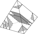
Figure 1: Several normal discs within a single tetrahedron

The triangles and quadrilaterals within a tetrahedron can be grouped into seven normal disc types, according to which edges of the tetrahedron they intersect. This includes four triangular disc types and three quadrilateral disc types, all of which are illustrated in Figure 2.

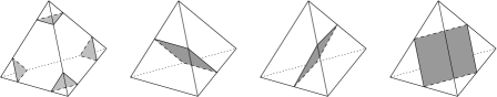
Figure 2: The seven different normal disc types within a tetrahedron

Equivalence of normal surfaces is defined by normal isotopy, which is an ambient isotopy that preserves each simplex of the triangulation $\mathcal{T}$. Throughout this paper, any two surfaces that are related by normal isotopy are regarded as the same surface.

Vertex links are normal surfaces that play an important role in the discussion that follows. If $V$ is a vertex of the triangulation $\mathcal{T}$ then the vertex link of $V$, denoted $\ell(V)$, is the normal surface at the frontier of a small regular neighbourhood of $V$. This surface is formed entirely from triangular discs (one copy of each triangular disc type surrounding $V$). Here we follow the nomenclature of Jaco and Rubinstein [15]; Tollefson refers to vertex links as trivial surfaces.

A core strength of normal surface theory is its ability to reduce difficult problems in topology to simpler problems in linear algebra. This is where the formulations of Haken and Tollefson differ, and so we slow down from here onwards to give full details. The key difference between the two formulations is that Haken works in a $7n$-dimensional vector space with coordinates based on triangle and quadrilateral disc types, whereas Tollefson works in a $3n$-dimensional space based on quadrilateral disc types only.

Definition 2.1 (Vector Representations)

Let $\mathcal{T}$ be a compact 3-manifold triangulation formed from the $n$ tetrahedra $\Delta_{1},\ldots,\Delta_{n}$, and let $S$ be an embedded normal surface in $\mathcal{T}$. For each tetrahedron $\Delta_{i}$, let $t_{i,1}$, $t_{i,2}$, $t_{i,3}$ and $t_{i,4}$ denote the number of triangular discs of $S$ of each type in $\Delta_{i}$, and let $q_{i,1}$, $q_{i,2}$ and $q_{i,3}$ denote the number of quadrilateral discs of $S$ of each type in $\Delta_{i}$.

Then the standard vector representation of $S$, denoted $\mathbf{v}(S)$, is the $7n$-dimensional vector

$$\mathbf{v}(S)~{}=\,\left(\ t_{1,1},t_{1,2},t_{1,3},t_{1,4},\ q_{1,1},q_{1,2},q_{1,3}\ ;\ t_{2,1},t_{2,2},t_{2,3},t_{2,4},\ q_{2,1},q_{2,2},q_{2,3}\ ;\ \ldots,q_{n,3}\ \right),$$

and the quadrilateral vector representation of $S$, denoted $\mathbf{q}(S)$, is the $3n$-dimensional vector

$$\mathbf{q}(S)~{}=\,\left(\ q_{1,1},q_{1,2},q_{1,3}\ ;\ q_{2,1},q_{2,2},q_{2,3}\ ;\ \ldots,q_{n,3}\ \right).$$

When we are working with $\mathbf{v}(S)$, we say we are working in standard coordinates (or standard normal coordinates if we wish to distinguish between normal and almost normal surfaces). Likewise, when working with $\mathbf{q}(S)$ we say we are working in quadrilateral coordinates. The following uniqueness results are due to Haken [8] and Tollefson [26]:

Lemma 2.2

Let $\mathcal{T}$ be a compact 3-manifold triangulation, and let $S$ and $S^{\prime}$ be embedded normal surfaces in $\mathcal{T}$.

• The standard vector representations $\mathbf{v}(S)$ and $\mathbf{v}(S^{\prime})$ are equal if and only if the surfaces $S$ and $S^{\prime}$ are normal isotopic (i.e., they are the “same” normal surface).

• The quadrilateral vector representations $\mathbf{q}(S)$ and $\mathbf{q}(S^{\prime})$ are equal if and only if either (i) $S$ and $S^{\prime}$ are normal isotopic, or (ii) $S$ and $S^{\prime}$ can be made normal isotopic by adding or removing vertex linking components.

Since we are rarely interested in vertex linking components, Lemma 2.2 shows that the standard and quadrilateral vector representations each contain everything we might want to know about an embedded normal surface.

Not every integer vector $\mathbf{w}\in\mathbb{R}^{7n}$ or $\mathbf{w}\in\mathbb{R}^{3n}$ is the vector representation of a normal surface. The necessary conditions on $\mathbf{w}$ include a set of matching equations as well as a set of quadrilateral constraints, which we define as follows.

Definition 2.3 (Standard Matching Equations)

Let $\mathcal{T}$ be a compact 3-manifold triangulation formed from the $n$ tetrahedra $\Delta_{1},\ldots,\Delta_{n}$, and let $\mathbf{w}\in\mathbb{R}^{7n}$ be any $7n$-dimensional vector whose coordinates we label

$$\mathbf{w}~{}=\,\left(\ t_{1,1},t_{1,2},t_{1,3},t_{1,4},\ q_{1,1},q_{1,2},q_{1,3}\ ;\ t_{2,1},t_{2,2},t_{2,3},t_{2,4},\ q_{2,1},q_{2,2},q_{2,3}\ ;\ \ldots,q_{n,3}\ \right).$$

For each non-boundary face of $\mathcal{T}$ and each of the three edges surrounding it, we obtain a standard matching equation on $\mathbf{w}$ as follows.

Let $F$ be some non-boundary face of $\mathcal{T}$, and let $e$ be one of the three edges surrounding $F$. Suppose that $\Delta_{i}$ and $\Delta_{j}$ are the two tetrahedra on either side of $F$. Then there is precisely one triangular disc type and one quadrilateral disc type in each of $\Delta_{i}$ and $\Delta_{j}$ that meets $F$ in an arc parallel to $e$, as illustrated in Figure 3. Suppose these disc types correspond to coordinates $t_{i,a}$, $q_{i,b}$, $t_{j,c}$ and $q_{j,d}$ respectively. Then we obtain the matching equation

$$t_{i,a}+q_{i,b}=t_{j,c}+q_{j,d}.$$

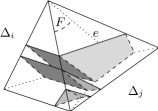
Figure 3: Building the standard matching equations

Essentially, the standard matching equations ensure that all of the normal discs on either side of a non-boundary face $F$ can be joined together. In Figure 3, the four coordinates are $(t_{i,a},q_{i,b},t_{j,c},q_{j,d})=(1,2,2,1)$, giving the equation $1+2=2+1$ which is indeed satisfied. If $\mathcal{T}$ is a closed triangulation (i.e., it has no boundary), then there are precisely $6n$ standard matching equations for $\mathcal{T}$ (three for each of the $2n$ faces of $\mathcal{T}$).

Definition 2.4 (Quadrilateral Matching Equations)

Let $\mathcal{T}$ be a compact 3-manifold triangulation formed from the $n$ tetrahedra $\Delta_{1},\ldots,\Delta_{n}$, and let $\mathbf{w}\in\mathbb{R}^{3n}$ be any $3n$-dimensional vector whose coordinates we label

$$\mathbf{w}~{}=\,\left(\ q_{1,1},q_{1,2},q_{1,3}\ ;\ q_{2,1},q_{2,2},q_{2,3}\ ;\ \ldots,q_{n,3}\ \right).$$

For each non-boundary edge of $\mathcal{T}$, we obtain a quadrilateral matching equation on $\mathbf{w}$ as follows.

Let $e$ be some non-boundary edge of $\mathcal{T}$, and arbitrarily label the two ends of $e$ as upper and lower. The tetrahedra containing edge $e$ are arranged in a cycle around $e$, as illustrated in Figure 4. Choose some arbitrary direction around this cycle, and suppose that the tetrahedra that we encounter as we travel in this direction around the cycle are labelled $\Delta_{i_{1}},\ldots,\Delta_{i_{t}}$.

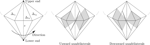
Figure 4: Building the quadrilateral matching equations

For each tetrahedron in this cycle, there are two quadrilateral types meeting edge $e$: one that rises from the lower end of $e$ to the upper as we travel around the cycle in the chosen direction, and one that falls from the upper end of $e$ to the lower. We call these the upward quadrilaterals and downward quadrilaterals respectively; these are again illustrated in Figure 4.

Suppose now that the coordinates corresponding to the upward and downward quadrilateral types are $q_{i_{1},u_{1}},q_{i_{2},u_{2}},\ldots,q_{i_{t},u_{t}}$ and $q_{i_{1},d_{1}},q_{i_{2},d_{2}},\ldots,q_{i_{t},d_{t}}$ respectively. Then we obtain the matching equation

$$q_{i_{1},u_{1}}+q_{i_{2},u_{2}}+\ldots+q_{i_{t},u_{t}}=q_{i_{1},d_{1}}+q_{i_{2},d_{2}}+\ldots+q_{i_{t},d_{t}}.$$ (2.1)

In other words, the total number of upward quadrilaterals surrounding $e$ equals the total number of downward quadrilaterals surrounding $e$.

Note that a single tetrahedron might appear multiple times in the cycle around $e$, in which case a single coordinate $q_{i,j}$ might appear more than once in the equation (2.1). For a closed triangulation $\mathcal{T}$ with $v$ vertices, a quick Euler characteristic calculation shows that we have precisely $n+v$ edges in our triangulation and therefore precisely $n+v$ quadrilateral matching equations.

Definition 2.5 (Quadrilateral Constraints)

Let $\mathcal{T}$ be a compact 3-manifold triangulation formed from the $n$ tetrahedra $\Delta_{1},\ldots,\Delta_{n}$, and consider any vector

$$\mathbf{w}~{} =\,\left(\ t_{1,1},t_{1,2},t_{1,3},t_{1,4},\ q_{1,1},q_{1,2},q_{1,3}\ ;\ \ldots,q_{n,3}\ \right)\in\mathbb{R}^{7n}\ \mbox{or}$$

$$\mathbf{w}~{} =\,\left(\ q_{1,1},q_{1,2},q_{1,3}\ ;\ \ldots,q_{n,3}\ \right)\in\mathbb{R}^{3n}.$$

We say that $\mathbf{w}$ satisfies the quadrilateral constraints if, for every tetrahedron $\Delta_{i}$, at most one of the quadrilateral coordinates $q_{i,1}$, $q_{i,2}$ and $q_{i,3}$ is non-zero.

We can now describe a full set of necessary and sufficient conditions for a vector $\mathbf{w}\in\mathbb{R}^{7n}$ or $\mathbf{w}\in\mathbb{R}^{3n}$ to be the vector representation of some embedded normal surface. The following result is due to Haken [8] and Tollefson [26].

Theorem 2.6

Let $\mathcal{T}$ be a compact 3-manifold triangulation formed from $n$ tetrahedra. An integer vector ($\mathbf{w}\in\mathbb{R}^{7n}$ or $\mathbf{w}\in\mathbb{R}^{3n}$) is the (standard or quadrilateral) vector representation of an embedded normal surface in $\mathcal{T}$ if and only if:

• The coordinates of $\mathbf{w}$ are all non-negative;

• $\mathbf{w}$ satisfies the (standard or quadrilateral) matching equations for $\mathcal{T}$;

• $\mathbf{w}$ satisfies the quadrilateral constraints for $\mathcal{T}$.

Such a vector is referred to as an admissible vector.

Essentially, the non-negativity constraint ensures that the coordinates of $\mathbf{w}$ can be used to count normal discs, the matching equations ensure that these discs can be joined together to form a surface, and the quadrilateral constraint ensures that this surface is embedded (since any two quadrilaterals of different types within the same tetrahedron must intersect).

Many high-level algorithms in 3-manifold topology involve the enumeration of vertex normal surfaces, which form a basis from which we can reconstruct all embedded normal surfaces within a triangulation $\mathcal{T}$. The relevant definitions are as follows.

Definition 2.7 (Projective Solution Space)

Let $\mathcal{T}$ be a compact 3-manifold triangulation formed from $n$ tetrahedra. The set of all non-negative vectors in $\mathbb{R}^{7n}$ that satisfy the standard matching equations for $\mathcal{T}$ forms a rational polyhedral cone in $\mathbb{R}^{7n}$. The standard projective solution space for $\mathcal{T}$ is the rational polytope formed by intersecting this cone with the hyperplane $\{\mathbf{w}\in\mathbb{R}^{7n}\,|\,\sum w_{i}=1\}$.

The quadrilateral projective solution space for $\mathcal{T}$ is defined in a similar fashion by working in $\mathbb{R}^{3n}$ and using the quadrilateral matching equations instead.

Definition 2.8 (Vertex Normal Surface)

Let $\mathcal{T}$ be a compact 3-manifold triangulation, and let $S$ be an embedded normal surface in $\mathcal{T}$. If the standard vector representation $\mathbf{v}(S)$ is a positive multiple of some vertex of the standard projective solution space, then we call $S$ a standard vertex normal surface. Likewise, if the quadrilateral vector representation $\mathbf{q}(S)$ is a positive multiple of some vertex of the quadrilateral projective solution space, then we call $S$ a quadrilateral vertex normal surface.

It should be noted that the definition of a vertex normal surface varies between authors. Definition 2.8 is consistent with Jaco and Rubinstein [15], as well as earlier work of this author [6]. Other authors impose additional conditions, such as Tollefson [26] who requires $S$ to be connected and two-sided, or Jaco and Oertel [14] who require the elements of $\mathbf{v}(S)$ to have no common factor (and who use the alternate name fundamental edge surface).

Although vertex normal surfaces can be used as a basis for reconstructing all embedded normal surfaces within a triangulation, this is typically not feasible since there are infinitely many such surfaces. Instead we frequently find that, when searching for an embedded normal surface with some desirable property, we can restrict our attention only to vertex normal surfaces. For instance, Jaco and Oertel [14] prove for closed irreducible 3-manifolds that if a two-sided incompressible surface exists then one can be found as a standard vertex normal surface. Likewise, Jaco and Tollefson [16] prove that if a 3-manifold contains an essential disc or sphere then one can be found as a standard vertex normal surface.

Using results of this type, a typical high-level algorithm based on normal surface theory includes the following steps:

1. Enumerate the (finitely many) vertices of the projective solution space for a given triangulation $\mathcal{T}$, using techniques from linear programming (see [5] for details).

2. Eliminate those vertices that do not satisfy the quadrilateral constraints, and then reconstruct the vertex normal surfaces of $\mathcal{T}$ by taking multiples of those vertices that remain. Although there are infinitely many such multiples, only finitely many will yield connected normal surfaces, which is typically what we are searching for.

3. Test each of these vertex normal surfaces for some desirable property (such as incompressibility, or being an essential disc or sphere).

Here we can see the real benefit of working in quadrilateral coordinates—the enumeration of step (i) takes place in a vector space of dimension $7n$ for standard coordinates, but only $3n$ for quadrilateral coordinates. Since both the running time and memory usage can become exponential in this dimension [5], a reduction from $7n$ to $3n$ can yield dramatic improvements in performance.

However, there is a trade-off for using quadrilateral coordinates. Although every connected quadrilateral vertex normal surface is also a standard vertex normal surface [6], the converse is not true in general. Instead, there might be standard vertex normal surfaces (perhaps including the incompressible surfaces, essential discs and spheres or whatever else we are searching for) that do not show up as quadrilateral vertex normal surfaces. These “lost surfaces” can undermine the correctness of our algorithms, which we maintain in one of two ways:

• We can resolve the problem using theory. This requires us to prove that, if the surface we are searching for exists, then it exists not only as a standard vertex normal surface but also as a quadrilateral vertex normal surface.

  Such results can be more difficult to prove in quadrilateral coordinates than in standard coordinates, partly because important functions such as Euler characteristic are no longer linear. Nevertheless, examples can be found—Tollefson [26] proves such a result for two-sided incompressible surfaces, and Jaco et al. [13] refer to similar results for essential discs and spheres.

• We can resolve the problem using algorithms and computation. There is a fast algorithm described in [6] that converts a full set of quadrilateral vertex normal surfaces to a full set of standard vertex normal surfaces, thereby recovering those surfaces that were lost. This algorithm is found to have a negligible running time, which means that we are able to work with standard vertex normal surfaces yet still enjoy the significantly greater performance of quadrilateral coordinates.

The main part of this paper is concerned with the development of quadrilateral-octagon coordinates for almost normal surfaces, where we face a similar trade-off. In Section 5 we resolve this problem for the 3-sphere recognition algorithm using the theoretical route, and in Section 6 we show how the more general algorithmic solution can be used.

3 Almost Normal Surfaces

Almost normal surfaces are an extension of normal surfaces whereby, in addition to the usual normal discs, we allow one tetrahedron of the triangulation to contain a single unusual intersection piece. Introduced by Rubinstein for use with the 3-sphere algorithm and related problems [20, 21], almost normal surfaces also enjoy other applications such as the determination of Heegaard genus [18], the recognition of small Seifert fibred spaces [22], and finding bridge surfaces in knot complements [27].

We begin this section by defining almost normal surfaces, whereupon we restrict our attention to octagonal almost normal surfaces. Octagonal almost normal surfaces are significantly easier to deal with, and Thompson has proven that they are sufficient for use with the 3-sphere recognition algorithm [23].

In the remainder of this section, we define concepts similar to those seen in Section 2, such as vector representation, matching equations and vertex almost normal surfaces. These concepts and their corresponding results are well-known extensions to traditional normal surface theory; see Lackenby [18] or Rubinstein [21] for a brief sketch. The details however are not explicitly laid down in the current literature, and so we present these details here.

Definition 3.1 (Almost Normal Surface)

Let $\mathcal{T}$ be a compact 3-manifold triangulation, and let $\Delta$ be some tetrahedron of $\mathcal{T}$. A normal octagon in $\Delta$ is a properly embedded disc in $\Delta$ whose boundary consists of eight normal arcs running across the faces of $\Delta$, as illustrated in Figure 5. A normal tube in $\Delta$ is a properly embedded annulus in $\Delta$ consisting of any two disjoint normal discs joined by an unknotted tube, again illustrated in Figure 5.

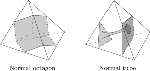
Figure 5: Examples of exceptional pieces in almost normal surfaces

An almost normal surface in $\mathcal{T}$ is a properly embedded surface whose intersection with the tetrahedra of $\mathcal{T}$ consists of (i) zero or more normal discs, plus (ii) in precisely one tetrahedron of $\mathcal{T}$, either a single normal octagon or a single normal tube (but not both). This single octagon or tube is referred to as the exceptional piece of the almost normal surface.

Although Definition 3.1 requires that almost normal surfaces be properly embedded, for brevity’s sake we do not include the word “embedded” in their name. For the remainder of this paper we concern ourselves only with octagonal almost normal surfaces, which are defined as follows.

Definition 3.2 (Octagonal Almost Normal Surface)

An octagonal almost normal surface is an almost normal surface whose exceptional piece is a normal octagon (not a tube). For contrast, we will often refer to the almost normal surfaces of Definition 3.1 (where the exceptional piece may be either an octagon or a tube) as general almost normal surfaces.

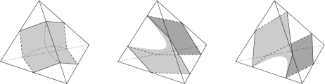
Figure 6: The three different octagon types within a tetrahedron

The possible normal octagons within a tetrahedron can be grouped into three octagon types, according to how many times they intersect each edge of the tetrahedron. All three octagon types are illustrated in Figure 6.

As with “embedded”, we will sometimes drop the word “octagonal” from definitions to avoid excessively long names; see for instance the standard almost normal matching equations and vertex almost normal surfaces (Definitions 3.3 and 3.5), which refer exclusively to octagonal almost normal surfaces.

At this early stage we can already see one reason why octagonal almost normal surfaces are substantially easier to deal with than general almost normal surfaces—while there are only three octagon types within a tetrahedron, there are $25$ distinct types of normal tube, giving $28$ types of exceptional piece in the general case. Not only is this messier to implement on a computer, but it can lead to significant increases in running time and memory usage. We return to this issue at the end of this section.

Definition 3.3 (Standard Vector Representation)

Let $\mathcal{T}$ be a compact 3-manifold triangulation formed from the $n$ tetrahedra $\Delta_{1},\ldots,\Delta_{n}$, and let $S$ be an octagonal almost normal surface in $\mathcal{T}$. For each tetrahedron $\Delta_{i}$, let $t_{i,1}$, $t_{i,2}$, $t_{i,3}$ and $t_{i,4}$ denote the number of triangular discs of each type, let $q_{i,1}$, $q_{i,2}$ and $q_{i,3}$ denote the number of quadrilateral discs of each type, and let $k_{i,1}$, $k_{i,2}$ and $k_{i,3}$ denote the number of octagonal discs of each type in $\Delta_{i}$ contained in the surface $S$.

Then the standard vector representation of $S$, denoted $\mathbf{v}(S)$, is the $10n$-dimensional vector

$$\mathbf{v}(S)~{}=\,(~{} t_{1,1},t_{1,2},t_{1,3},t_{1,4},\ q_{1,1},q_{1,2},q_{1,3},\ k_{1,1},k_{1,2} ,k_{1,3}\ ;$$

$$t_{2,1},t_{2,2},t_{2,3},t_{2,4},\ q_{2,1},q_{2,2},q_{2,3},\ k_{2,1},k_{2,2} ,k_{2,3}\ ;$$

$$\ldots ,k_{n,3}\ ).$$

Lemma 3.4

Let $\mathcal{T}$ be a compact 3-manifold triangulation, and let $S$ and $S^{\prime}$ be octagonal almost normal surfaces in $\mathcal{T}$. Then the standard vector representations $\mathbf{v}(S)$ and $\mathbf{v}(S^{\prime})$ are equal if and only if the surfaces $S$ and $S^{\prime}$ are normal isotopic (i.e., they are the “same” almost normal surface).

This result is the almost normal counterpart to Lemma 2.2. The proof is the same, and so we do not present the details here. The key observation is that, given some number of triangles, quadrilaterals and/or octagons of various types in a single tetrahedron, if these discs can be packed into the tetrahedron disjointly then this packing is unique up to normal isotopy.

This brings us to another reason why octagonal almost normal surfaces are simpler to deal with than general almost normal surfaces. In the general case, this packing need not be unique. In particular, a tube that joins two normal discs of the same type can be interchanged with some other normal disc of the same type without creating intersections (see Figure 7 for an illustration). Because of this, the extension of Lemma 3.4 to general almost normal surfaces fails to hold.

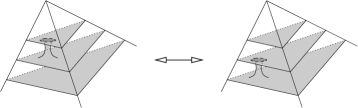
Figure 7: Packing a triangle and a tube into a tetrahedron in two distinct ways

To determine precisely which vectors in $\mathbb{R}^{10n}$ represent octagonal almost normal surfaces, we develop a set of matching equations and quadrilateral-octagon constraints in a similar fashion to Definitions 2.3 and 2.5.

Definition 3.5 (Standard Almost Normal Matching Equations)

Let $\mathcal{T}$ be a compact 3-manifold triangulation formed from the $n$ tetrahedra $\Delta_{1},\ldots,\Delta_{n}$, and let $\mathbf{w}\in\mathbb{R}^{10n}$ be any $10n$-dimensional vector whose coordinates we label

$$\mathbf{w}~{}=\,\left(\ t_{1,1},t_{1,2},t_{1,3},t_{1,4},\ q_{1,1},q_{1,2},q_{1,3},\ k_{1,1},k_{1,2},k_{1,3}\ ;\ \ldots,k_{n,3}\ \right).$$

For each non-boundary face of $\mathcal{T}$ and each of the three edges surrounding it, we obtain a standard almost normal matching equation on $\mathbf{w}$ as follows.

Let $F$ be some non-boundary face of $\mathcal{T}$, and let $e$ be one of the three edges surrounding $F$. Suppose that $\Delta_{i}$ and $\Delta_{j}$ are the two tetrahedra on either side of $F$. Precisely one triangular disc type, one quadrilateral disc type and two octagonal disc types in each of $\Delta_{i}$ and $\Delta_{j}$ meet $F$ in an arc parallel to $e$. Suppose these correspond to coordinates $t_{i,a}$, $q_{i,b}$, $k_{i,c}$ and $k_{i,d}$ for $\Delta_{i}$ and $t_{j,e}$, $q_{j,f}$, $k_{j,g}$ and $k_{j,h}$ for $\Delta_{j}$. Then we obtain the matching equation

$$t_{i,a}+q_{i,b}+k_{i,c}+k_{i,d}=t_{j,e}+q_{j,f}+k_{j,g}+k_{j,h}.$$ (3.2)

These matching equations are the obvious extension to the original standard matching equations of Definition 2.3—we ensure that all of the discs on one side of a non-boundary face can be joined to all of the discs on the other side. As with normal surfaces, if $\mathcal{T}$ is a closed triangulation then there are precisely $6n$ standard almost normal matching equations (three for each of the $2n$ faces of $\mathcal{T}$).

Definition 3.6 (Quadrilateral-Octagon Constraints)

Let $\mathcal{T}$ be a compact 3-manifold triangulation formed from the $n$ tetrahedra $\Delta_{1},\ldots,\Delta_{n}$, and consider any vector

$$\mathbf{w}~{}=\,\left(\ t_{1,1},t_{1,2},t_{1,3},t_{1,4},\ q_{1,1},q_{1,2},q_{1,3},\ k_{1,1},k_{1,2},k_{1,3}\ ;\ \ldots,k_{n,3}\ \right)\in\mathbb{R}^{10n}.$$

We say that $\mathbf{w}$ satisfies the quadrilateral-octagon constraints if and only if:

1. For every tetrahedron $\Delta_{i}$, at most one of the six quadrilateral and octagonal coordinates $q_{i,1}$, $q_{i,2}$, $q_{i,3}$, $k_{i,1}$, $k_{i,2}$ and $k_{i,3}$ is non-zero;

2. In the entire triangulation $\mathcal{T}$, at most one of the $3n$ octagonal coordinates $k_{1,1},\ldots,k_{n,3}$ is non-zero.

Like the quadrilateral constraints of Definition 2.5, condition (i) of the quadrilateral-octagon constraints ensures that the discs within a single tetrahedron can be embedded without intersecting. Condition (ii) ensures that we have at most one octagon type within a triangulation—although this condition is not strong enough to ensure at most one octagonal disc, it does have the useful property of invariance under scalar multiplication.

Note that a vector can still satisfy the quadrilateral-octagon constraints even if all its octagonal coordinates are zero. This is necessary for the vertex enumeration algorithms to function properly; we return to this issue in Section 6.

We can now give a full set of necessary and sufficient conditions for a vector in $\mathbb{R}^{10n}$ to represent an octagonal almost normal surface.

Theorem 3.7

Let $\mathcal{T}$ be a compact 3-manifold triangulation formed from $n$ tetrahedra. An integer vector $\mathbf{w}\in\mathbb{R}^{10n}$ is the standard vector representation of an octagonal almost normal surface in $\mathcal{T}$ if and only if:

• The coordinates of $\mathbf{w}$ are all non-negative;

• $\mathbf{w}$ satisfies the standard almost normal matching equations for $\mathcal{T}$;

• $\mathbf{w}$ satisfies the quadrilateral-octagon constraints for $\mathcal{T}$;

• There is precisely one non-zero octagonal coordinate in $\mathbf{w}$, and this coordinate is set to one.

Once again, such a vector is called an admissible vector.

Again the proof is essentially the same as for the corresponding theorem in normal surface theory (Theorem 2.6), and so we do not reiterate the details here. The only difference is that we now have a global condition in the quadrilateral-octagon constraints (at most one non-zero octagonal coordinate in the entire triangulation), as well as an extra constraint for admissibility (precisely one non-zero octagonal coordinate with value one). These are to satisfy Definition 3.1, which requires an almost normal surface to have precisely one exceptional piece.

It is occasionally useful to consider surfaces with any number of octagonal discs, though still at most one octagonal disc type. In this case the vector representation, matching equations and quadrilateral-octagon constraints all remain the same; the only change appears in Theorem 3.7, where we remove the final condition (the one that requires a unique non-zero octagonal coordinate with a value of one).

We finish by defining a vertex almost normal surface in a similar fashion to Definition 2.8. We are careful here to specify our coordinate system—in Section 4 we define a similar concept in quadrilateral-octagon coordinates, and (as with normal surfaces) a vertex surface in one coordinate system need not be a vertex surface in another.

Definition 3.8 (Standard Vertex Almost Normal Surface)

Let $\mathcal{T}$ be a compact 3-manifold triangulation formed from $n$ tetrahedra. The standard almost normal projective solution space for $\mathcal{T}$ is the rational polytope formed by (i) taking the polyhedral cone of all non-negative vectors in $\mathbb{R}^{10n}$ that satisfy the standard almost normal matching equations for $\mathcal{T}$, and then (ii) intersecting this cone with the hyperplane $\{\mathbf{w}\in\mathbb{R}^{10n}\,|\,\sum w_{i}=1\}$.

Let $S$ be an octagonal almost normal surface in $\mathcal{T}$. If the standard vector representation $\mathbf{v}(S)$ is a positive multiple of some vertex of the standard almost normal projective solution space, then we call $S$ a standard vertex almost normal surface.

As with normal surfaces, we can use the enumeration of vertex almost normal surfaces as a basis for high-level topological algorithms. The streamlined 3-sphere recognition of Jaco, Rubinstein and Thompson [15] does just this—given a “sufficiently nice” 3-manifold triangulation $\mathcal{T}$, we (i) enumerate all standard vertex almost normal surfaces within $\mathcal{T}$, and then (ii) search amongst these vertex surfaces for an almost normal 2-sphere. We return to this algorithm in detail in Section 5.

This suggests yet another reason to prefer octagonal almost normal surfaces over general almost normal surfaces. Whereas octagonal almost normal surfaces have $10n$-dimensional vector representations, in the general case we would need $35n$ dimensions (allowing for $25$ types of tube in addition to the ten octagons, quadrilaterals and triangles in each tetrahedron). Since both the running time and memory usage for vertex enumeration can grow exponential in the dimension of the underlying vector space [5], increasing this dimension from $10n$ to $35n$ could well have a crippling effect on performance.

4 Quadrilateral-Octagon Coordinates

At this stage we are ready to develop quadrilateral-octagon coordinates, which form the main focus of this paper. Quadrilateral-octagon coordinates act as an almost normal analogy to Tollefson’s quadrilateral coordinates, in that we “forget” all information regarding triangular discs. As with quadrilateral coordinates, we happily find that—except for vertex linking components—all of the forgotten information can be successfully recovered.

The main results of this section are (i) to show that vectors in quadrilateral-octagon coordinates uniquely identify surfaces up to vertex linking components (Lemma 4.2), and (ii) to develop a set of necessary and sufficient conditions for a vector in quadrilateral-octagon coordinates to represent an octagonal almost normal surface (Theorem 4.5). Although these mirror Tollefson’s original results in quadrilateral coordinates, the proofs follow a different course—in this sense the author hopes that this paper and Tollefson’s paper [26] make complementary reading.

Definition 4.1 (Quadrilateral-Octagon Vector Representation)

Let $\mathcal{T}$ be a compact 3-manifold triangulation formed from the $n$ tetrahedra $\Delta_{1},\ldots,\Delta_{n}$, and let $S$ be an octagonal almost normal surface in $\mathcal{T}$. For each tetrahedron $\Delta_{i}$, let $q_{i,1}$, $q_{i,2}$ and $q_{i,3}$ denote the number of quadrilateral discs of each type, and let $k_{i,1}$, $k_{i,2}$ and $k_{i,3}$ denote the number of octagonal discs of each type in $\Delta_{i}$ contained in the surface $S$.

Then the quadrilateral-octagon vector representation of $S$, denoted $\mathbf{k}(S)$, is the $6n$-dimensional vector

$$\mathbf{k}(S)~{}=\,\left(~{}q_{1,1},q_{1,2},q_{1,3},\ k_{1,1},k_{1,2},k_{1,3}\ ;\ q_{2,1},q_{2,2},q_{2,3},\ k_{2,1},k_{2,2},k_{2,3}\ ;\ \ldots,k_{n,3}\ \right).$$

Our first result in quadrilateral-octagon coordinates is a uniqueness lemma, analogous to Lemma 2.2 for normal surfaces and Lemma 3.4 for standard almost normal coordinates.

Lemma 4.2

Let $\mathcal{T}$ be a compact 3-manifold triangulation, and let $S$ and $S^{\prime}$ be octagonal almost normal surfaces in $\mathcal{T}$. Then the quadrilateral-octagon vector representations $\mathbf{k}(S)$ and $\mathbf{k}(S^{\prime})$ are equal if and only if either (i) the surfaces $S$ and $S^{\prime}$ are normal isotopic, or (ii) $S$ and $S^{\prime}$ can be made normal isotopic by adding or removing vertex linking components.

Proof.

The “if” direction is straightforward. If $S$ and $S^{\prime}$ are normal isotopic or can be made so by adding or removing vertex linking components, it follows from Lemma 3.4 that their standard vector representations $\mathbf{v}(S)$ and $\mathbf{v}(S^{\prime})$ differ only in their triangular coordinates (since vertex links consist entirely of triangular discs). Therefore the quadrilateral and octagonal coordinates are identical in both $\mathbf{v}(S)$ and $\mathbf{v}(S^{\prime})$, and we have $\mathbf{k}(S)=\mathbf{k}(S^{\prime})$.

For the “only if” direction, suppose that $\mathbf{k}(S)=\mathbf{k}(S^{\prime})$. Let $\mathbf{d}=\mathbf{v}(S)-\mathbf{v}(S^{\prime})$ in standard almost normal coordinates; it follows then that

$$\mathbf{d}~{}=\,\left(\ t_{1,1},t_{1,2},t_{1,3},t_{1,4},\ 0,0,0,\ 0,0,0\ ;\ t_{2,1},t_{2,2},t_{2,3},t_{2,4},\ 0,0,0,\ 0,0,0\ ;\ \ldots\ \right)\in\mathbb{R}^{10n}$$

for some set of triangular coordinates $\{t_{i,j}\}$. In other words, all of the quadrilateral and octagonal coordinates of $\mathbf{d}$ are zero.

We know from Theorem 2.6 that $\mathbf{v}(S)$ and $\mathbf{v}(S^{\prime})$ both satisfy the standard almost normal matching equations, and because these equations are linear it follows that $\mathbf{d}$ satisfies them also. However, with the quadrilateral and octagonal coordinates of $\mathbf{d}$ equal to zero, we find that each matching equation (3.2) reduces to the form $t_{i,a}=t_{j,e}$, where $t_{i,a}$ and $t_{j,e}$ represent triangular disc types surrounding a common vertex of the triangulation in adjacent tetrahedra (illustrated in Figure 8).

Figure 8: Adjacent triangles surrounding a common vertex

By following these matching equations around each vertex of the triangulation $\mathcal{T}$, we find that for each vertex $V$ of $\mathcal{T}$, the coordinates $\{t_{i,j}\}$ for all triangular disc types surrounding $V$ are equal. That is, $\mathbf{d}=\mathbf{v}(S)-\mathbf{v}(S^{\prime})$ is a linear combination of standard almost normal vector representations of vertex links. It follows then from Theorem 3.7 that the surfaces $S$ and $S^{\prime}$ can be made normal isotopic only by adding or removing vertex linking components. ∎

Following the pattern established in previous sections, we now turn our attention to building a set of necessary and sufficient conditions for a $6n$-dimensional vector to represent an almost normal surface in quadrilateral-octagon coordinates. These conditions include a set of matching equations modelled on the original quadrilateral matching equations of Tollefson (Definition 4.3), and a recasting of the quadrilateral-octagon constraints in $6n$ dimensions (Definition 4.4). The full set of necessary and sufficient conditions is laid down and proven in Theorem 4.5.

Definition 4.3 (Quadrilateral-Octagon Matching Equations)

Let $\mathcal{T}$ be a compact 3-manifold triangulation formed from the $n$ tetrahedra $\Delta_{1},\ldots,\Delta_{n}$, and let $\mathbf{w}\in\mathbb{R}^{6n}$ be any $6n$-dimensional vector whose coordinates we label

$$\mathbf{w}~{}=\,\left(\ q_{1,1},q_{1,2},q_{1,3},\ k_{1,1},k_{1,2},k_{1,3}\ ;\ \ldots,k_{n,3}\ \right).$$

For each non-boundary edge of $\mathcal{T}$, we obtain a quadrilateral-octagon matching equation on $\mathbf{w}$ as follows.

Let $e$ be some non-boundary edge of $\mathcal{T}$. As with Tollefson’s original quadrilateral matching equations, we arbitrarily label the two ends of $e$ as upper and lower. The tetrahedra containing edge $e$ are arranged in a cycle around $e$, as illustrated in the leftmost diagram of Figure 9. Choose some arbitrary direction around this cycle, and suppose that the tetrahedra that we encounter as we travel in this direction around the cycle are labelled $\Delta_{i_{1}},\ldots,\Delta_{i_{t}}$.

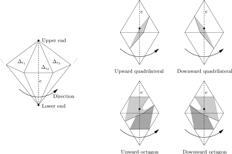
Figure 9: Building the quadrilateral-octagon matching equations

Consider any tetrahedron $\Delta_{i_{j}}$ in this cycle. Within this tetrahedron, there are two quadrilateral types and two octagon types that meet edge $e$ precisely once. For one quadrilateral and one octagon type, the intersection with $e$ acts as a “hinge” about which two adjacent edges of the disc rise from the lower end of $e$ to the upper end of $e$ as we travel around the cycle in the chosen direction. We call these disc types the upward quadrilateral and the upward octagon in $\Delta_{i_{j}}$, and we call the remaining two disc types the downward quadrilateral and the downward octagon in $\Delta_{i_{j}}$. All four disc types are illustrated in the rightmost portion of Figure 9.

Suppose now that the coordinates corresponding to the upward quadrilateral and octagon types are $q_{i_{1},u_{1}},q_{i_{2},u_{2}},\ldots,q_{i_{t},u_{t}}$ and $k_{i_{1},u_{1}^{\prime}},k_{i_{2},u_{2}^{\prime}},\ldots,k_{i_{t},u_{t}^{\prime}}$ respectively, and that the coordinates corresponding to the downward quadrilateral and octagon types are $q_{i_{1},d_{1}},q_{i_{2},d_{2}},\ldots,q_{i_{t},d_{t}}$ and $k_{i_{1},d_{1}^{\prime}},\allowbreak k_{i_{2},d_{2}^{\prime}},\ldots,k_{i_{t},d_{t}^{\prime}}$ respectively. Then we obtain the matching equation

$$q_{i_{1},u_{1}}+\ldots+q_{i_{t},u_{t}}+k_{i_{1},u_{1}^{\prime}}+\ldots+k_{i_{t},u_{t}^{\prime}}=q_{i_{1},d_{1}}+\ldots+q_{i_{t},d_{t}}+k_{i_{1},d_{1}^{\prime}}+\ldots+k_{i_{t},d_{t}^{\prime}}.$$ (4.3)

In other words, the total number of upward quadrilaterals and octagons surrounding $e$ equals the total number of downward quadrilaterals and octagons surrounding $e$.

Note that each tetrahedron surrounding $e$ contains a third quadrilateral type and a third octagon type, neither of which appears in equation (4.3). The third quadrilateral type is missing because it does not intersect with the edge $e$ at all. The third octagon type is missing because, although it intersects $e$ twice, these intersections behave in a similar fashion to two triangular discs (one at each end of $e$). Details can be found in the proof of Theorem 4.5.

As with Tollefson’s original quadrilateral matching equations, if our triangulation $\mathcal{T}$ is closed and has precisely $v$ vertices then we obtain a total of $n+v$ quadrilateral-octagon matching equations (one for each of the $n+v$ edges of $\mathcal{T}$).

Definition 4.4 (Quadrilateral-Octagon Constraints)

Let $\mathcal{T}$ be a compact 3-manifold triangulation formed from the $n$ tetrahedra $\Delta_{1},\ldots,\Delta_{n}$, and consider any vector

$$\mathbf{w}~{}=\,\left(\ q_{1,1},q_{1,2},q_{1,3},\ k_{1,1},k_{1,2},k_{1,3}\ ;\ \ldots,k_{n,3}\ \right)\in\mathbb{R}^{6n}.$$

We say that $\mathbf{w}$ satisfies the quadrilateral-octagon constraints if and only if:

1. For every tetrahedron $\Delta_{i}$, at most one of the six quadrilateral and octagonal coordinates $q_{i,1}$, $q_{i,2}$, $q_{i,3}$, $k_{i,1}$, $k_{i,2}$ and $k_{i,3}$ is non-zero;

2. In the entire triangulation $\mathcal{T}$, at most one of the $3n$ octagonal coordinates $k_{1,1},\ldots,k_{n,3}$ is non-zero.

Note that Definition 4.4 is essentially a direct copy of the quadrilateral-octagon constraints for standard almost normal coordinates (Definition 3.6), merely recast in $6n$ dimensions instead of $10n$.

We can now describe the full set of necessary and sufficient conditions for a vector to represent an almost normal surface in quadrilateral-octagon coordinates. The resulting theorem incorporates aspects of both Theorem 2.6 (which uses Tollefson’s original quadrilateral matching equations) and Theorem 3.7 (which introduces the quadrilateral-octagon constraints).

Theorem 4.5

Let $\mathcal{T}$ be a compact 3-manifold triangulation formed from $n$ tetrahedra. An integer vector $\mathbf{w}\in\mathbb{R}^{6n}$ is the quadrilateral-octagon vector representation of an octagonal almost normal surface in $\mathcal{T}$ if and only if:

• The coordinates of $\mathbf{w}$ are all non-negative;

• $\mathbf{w}$ satisfies the quadrilateral-octagon matching equations for $\mathcal{T}$;

• $\mathbf{w}$ satisfies the quadrilateral-octagon constraints for $\mathcal{T}$;

• There is precisely one non-zero octagonal coordinate in $\mathbf{w}$, and this coordinate is set to one.

Yet again, such a vector is called an admissible vector.

Proof.

We begin by showing that the four conditions listed in Theorem 4.5 are necessary. Let $S$ be some octagonal almost normal surface in $\mathcal{T}$. It is clear from Theorem 3.7 that the quadrilateral-octagon vector representation $\mathbf{k}(S)$ is a non-negative vector that satisfies the quadrilateral-octagon constraints, and that there is precisely one non-zero octagonal coordinate in $\mathbf{k}(S)$ whose value is set to one. All that remains then is to show that $\mathbf{k}(S)$ satisfies the quadrilateral-octagon matching equations, which is a simple matter of combining the standard almost normal matching equations appropriately. The details are as follows.

Suppose that $S$ has standard vector representation

$$\mathbf{v}(S)~{}=\,\left(\ t_{1,1},t_{1,2},t_{1,3},t_{1,4},\ q_{1,1},q_{1,2},q_{1,3},\ k_{1,1},k_{1,2},k_{1,3}\ ;\ \ldots,k_{n,3}\ \right).$$

Let $e$ be any non-boundary edge of $\mathcal{T}$, and arbitrarily label the two ends of $e$ as upper and lower. Following Definition 4.3, let the tetrahedra containing $e$ be labelled $\Delta_{i_{1}},\ldots,\Delta_{i_{t}}$ as we cycle in some arbitrary direction around $e$, let coordinates $q_{i_{1},u_{1}},q_{i_{2},u_{2}},\ldots,q_{i_{t},u_{t}}$ and $k_{i_{1},u_{1}^{\prime}},k_{i_{2},u_{2}^{\prime}},\ldots,k_{i_{t},u_{t}^{\prime}}$ correspond to the upward quadrilateral and octagon types, and let coordinates $q_{i_{1},d_{1}},q_{i_{2},d_{2}},\ldots,q_{i_{t},d_{t}}$ and $k_{i_{1},d_{1}^{\prime}},k_{i_{2},d_{2}^{\prime}},\ldots,k_{i_{t},d_{t}^{\prime}}$ correspond to the downward quadrilateral and octagon types.

We continue labelling coordinates as follows. Suppose that $t_{i_{1},a_{1}},t_{i_{1},a_{2}},\ldots,t_{i_{1},a_{t}}$ correspond to the triangular disc types surrounding the upper end of $e$, as illustrated in the left-hand portion of Figure 10. Furthermore, suppose that $k_{i_{1},b_{1}},k_{i_{2},b_{2}},\ldots,k_{i_{t},b_{t}}$ correspond to the octagonal disc types in each tetrahedron that are neither upward nor downward octagons, as illustrated in the right-hand portion of Figure 10.

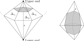
Figure 10: Triangles and octagons for the coordinates $t_{i_{j},a_{j}}$ and $k_{i_{j},b_{j}}$

Calling on Theorem 3.7 again, we know that $\mathbf{v}(S)$ satisfies the standard almost normal matching equations (Definition 3.5). Amongst those matching equations that involve the adjacent pairs of tetrahedra $(\Delta_{i_{1}},\Delta_{i_{2}})$, $(\Delta_{i_{2}},\Delta_{i_{3}})$, …, $(\Delta_{i_{t}},\Delta_{i_{1}})$, we find the $t$ equations

$$\begin{split}t_{i_{1},a_{1}}+q_{i_{1},u_{1}}+k_{i_{1},u_{1}^{\prime}}+k_{i_{1},b_{1}}&=t_{i_{2},a_{2}}+q_{i_{2},d_{2}}+k_{i_{2},d_{2}^{\prime}}+k_{i_{2},b_{2}},\\ t_{i_{2},a_{2}}+q_{i_{2},u_{2}}+k_{i_{2},u_{2}^{\prime}}+k_{i_{2},b_{2}}&=t_{i_{3},a_{3}}+q_{i_{3},d_{3}}+k_{i_{3},d_{3}^{\prime}}+k_{i_{3},b_{3}},\\ &\ \,\vdots\\ t_{i_{t},a_{t}}+q_{i_{t},u_{t}}+k_{i_{t},u_{t}^{\prime}}+k_{i_{t},b_{t}}&=t_{i_{1},a_{1}}+q_{i_{1},d_{1}}+k_{i_{1},d_{1}^{\prime}}+k_{i_{1},b_{1}}.\end{split}$$ (4.4)

Summing these together and cancelling the common terms $\{t_{i_{j},a_{j}}\}$ and $\{k_{i_{j},b_{j}}\}$, we obtain

$$q_{i_{1},u_{1}}+\ldots+q_{i_{t},u_{t}}+k_{i_{1},u_{1}^{\prime}}+\ldots+k_{i_{t},u_{t}^{\prime}}=q_{i_{1},d_{1}}+\ldots+q_{i_{t},d_{t}}+k_{i_{1},d_{1}^{\prime}}+\ldots+k_{i_{t},d_{t}^{\prime}}.$$

That is, the quadrilateral-octagon vector representation $\mathbf{k}(S)$ satisfies the quadrilateral-octagon matching equations.

We now turn to the more interesting task of proving that our list of conditions is sufficient for an integer vector $\mathbf{w}\in\mathbb{R}^{6n}$ to represent an octagonal almost normal surface. Let

$$\mathbf{w}~{}=\,\left(\ q_{1,1},q_{1,2},q_{1,3},\ k_{1,1},k_{1,2},k_{1,3}\ ;\ \ldots,k_{n,3}\ \right)\in\mathbb{R}^{6n}$$

be an arbitrary integer vector that satisfies the four conditions listed in the statement of this theorem. Our aim is to extend $\mathbf{w}$ to an integer vector

$$\mathbf{w}^{\prime}~{}=\,\left(\ t_{1,1},t_{1,2},t_{1,3},t_{1,4},\ q_{1,1},q_{1,2},q_{1,3},\ k_{1,1},k_{1,2},k_{1,3}\ ;\ \ldots,k_{n,3}\ \right)\in\mathbb{R}^{10n}$$

that satisfies the conditions of Theorem 3.7. If we can do this, it will follow from Theorem 3.7 that $\mathbf{w}^{\prime}$ is the standard almost normal vector representation of some octagonal almost normal surface in $\mathcal{T}$, whereupon $\mathbf{w}$ must be the quadrilateral-octagon vector representation of this same surface.

Given our conditions on $\mathbf{w}\in\mathbb{R}^{6n}$, it is clear that any non-negative extension $\mathbf{w}^{\prime}\in\mathbb{R}^{10n}$ will satisfy the quadrilateral-octagon constraints, and will have precisely one non-zero octagonal coordinate whose value is set to one. All we must do then is show that we can find a set of non-negative triangular coordinates $\{t_{i,j}\}$ that satisfy the standard almost normal matching equations of Definition 3.5.

Our broad strategy is to use the vertex links of $\mathcal{T}$ as a “canvas” on which we write the triangular coordinates $t_{i,j}$, and to reformulate the matching equations as local constraints on this canvas. In doing this, we show that the standard almost normal matching equations describe a cochain $\alpha\in C^{1}(\mathcal{D})$, where $\mathcal{D}$ is the dual polygonal decomposition of the vertex links, and that a solution $\{t_{i,j}\}$ exists if and only if $\alpha$ is a coboundary. Using the quadrilateral-octagon matching equations we then find that $\alpha$ is a cocycle, whereupon the result follows from the trivial homology of the vertex links. The details are as follows.

Because $\mathcal{T}$ is a compact triangulation, each of its vertex links is a triangulated sphere or disc, as illustrated in the left-hand diagram of Figure 11. Each triangular disc type appears once and only once amongst the vertex links, and so we can write each integer $t_{i,j}$ on the corresponding vertex link triangle as illustrated in the right-hand diagram of Figure 11. This is the sense in which we use the vertex links as a “canvas”.

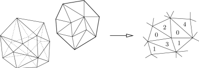
Figure 11: Writing the coordinates $t_{i,j}$ on the triangulated vertex links

We can now reformulate the standard almost normal matching equations as constraints on this canvas. Recall that each standard matching equation involves a face $F$ of $\mathcal{T}$ and arcs parallel to some edge $e$ of this face, as illustrated in the left-hand diagram of Figure 12. We can associate every such equation with a single non-boundary edge $g$ of a triangulated vertex link, where this edge $g$ also appears as an arc of the face $F$ parallel to $e$, as illustrated in the right-hand diagram of Figure 12. In this way, the standard almost normal matching equations and the non-boundary edges of the triangulated vertex links are in one-to-one correspondence.

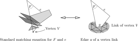
Figure 12: Associating a standard matching equation with an edge of a vertex link

Now consider some standard matching equation $t_{i,a}+q_{i,b}+k_{i,c}+k_{i,d}=t_{j,e}+q_{j,f}+k_{j,g}+k_{j,h}$ (as seen in Definition 3.5), and let $g$ be the corresponding edge of the triangulated vertex links. The coordinates $t_{i,a}$ and $t_{j,e}$ correspond to the triangles on either side of $g$, and so we can write this equation in the form

$$t_{i,a}-t_{j,e}=K,$$

where $K$ depends only on the quadrilateral and octagonal coordinates of $\mathbf{w}$. In other words, $K$ is a fixed quantity (dependent on the chosen edge $g$) that we can evaluate by looking at our original vector $\mathbf{w}\in\mathbb{R}^{6n}$. We express this equation on our canvas by drawing an arrow from the triangle containing $t_{j,e}$ to the triangle containing $t_{i,a}$, and by labelling this arrow with the constant $K$. This procedure is illustrated in Figure 13.

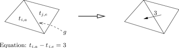
Figure 13: Representing a standard matching equation by a labelled arrow

Our situation is now as follows. On our canvas—the triangulated vertex links of $\mathcal{T}$—we have a labelled arrow crossing each non-boundary edge, and our task is to fill each triangle with an integer such that the difference across each edge matches the label on the corresponding arrow. An example of such a solution for a triangulated disc is illustrated in Figure 14. It is clear at this point that we do not need to worry about our non-negativity condition, since we can always add a constant to every triangle without changing the differences across the edges.

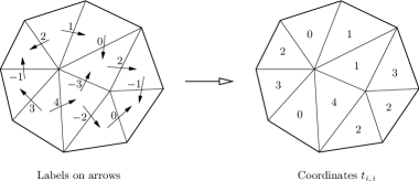
Figure 14: Solving the standard matching equations

We can rephrase this using the language of cohomology. Let $\mathcal{D}$ be the dual polygonal decomposition of the set of all vertex links, so that each triangle of a vertex link becomes a vertex of $\mathcal{D}$ and each labelled arrow becomes a directed edge of $\mathcal{D}$. Then together the arrows describe a cochain $\alpha\in C^{1}(\mathcal{D})$ that maps each dual edge to the corresponding label. A solution $\{t_{i,j}\}$ corresponds to a cochain $\beta\in C^{0}(\mathcal{D})$ that maps each dual vertex to the integer in the corresponding triangle, and the “difference condition” that such a solution must satisfy is simply $\alpha=\delta\beta$. That is, a solution $\{t_{i,j}\}$ exists if and only if $\alpha$ is a coboundary.

We now turn to the quadrilateral-octagon matching equations, which we assume hold for our original vector $\mathbf{w}\in\mathbb{R}^{6n}$. These equations do not involve the triangular coordinates at all. Instead they tell us about the relations between different quadrilateral and octagonal coordinates of $\mathbf{w}$, which means they give us information about the labels on our arrows.

Consider some vertex $V$ of the triangulation $\mathcal{T}$, let $U$ be some non-boundary vertex of the triangulated link $\ell(V)$, and let $e$ be the edge of $\mathcal{T}$ that runs through $U$ and $V$ as illustrated in Figure 15. Let $K_{1},\ldots,K_{t}$ be the labels on the arrows surrounding $U$, as seen in the right-hand diagram of this figure (where we make all arrows point in the same direction around $U$ by reversing arrows and negating labels as necessary). Recall that by construction, each label $K_{i}$ is a linear combination of two quadrilateral and four octagonal coordinates of $\mathbf{w}$.

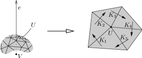
Figure 15: The triangles surrounding some vertex $U$ of the vertex link $\ell(V)$

Now consider the quadrilateral-octagon matching equation constructed from edge $e$. By declaring $V$ to be at the upper end of $e$, we can invert the procedure used earlier in equation (4.4) to express our matching equation as

$$K_{1}+\ldots+K_{t}=0.$$

In other words, the quadrilateral-octagon matching equations tell us that around every non-boundary vertex of a triangulated vertex link, the sum of labels on arrows is zero. We see this for instance in Figure 14—by walking clockwise around each internal vertex and negating labels when arrows point backwards, the left internal vertex gives $1+0-(-3)-4+3+(-1)-2=0$, and the right internal vertex gives $2+(-1)-0-(-2)+(-3)=0$.

Returning to our cohomology formulation, this simply tells us that $\delta\alpha=0$, where $\alpha\in C^{1}(\mathcal{D})$ is the cochain described earlier. That is, $\alpha$ is a cocycle. However, because each vertex link is a sphere or a disc, the cohomology group $H^{1}(\mathcal{D})$ is trivial. Therefore $\alpha$ is also a coboundary, as required. ∎

The final step of this proof shows why we must exclude the ideal triangulations of Thurston [24] from our consideration. In an ideal triangulation, vertices form higher-genus cusps, whereupon the vertex links become higher-genus surfaces with non-trivial homology. Therefore, although the quadrilateral-octagon matching equations still show that $\alpha\in C^{1}(\mathcal{D})$ is a cocycle in the proof above, we can no longer conclude from this that $\alpha$ is a coboundary and that the solution $\{t_{i,j}\}$ exists.

To finish this section, we define a vertex surface in our new coordinate system using the same pattern that we have employed several times already.

Definition 4.6 (Quadrilateral-Octagon Vertex Almost Normal Surface)

Let $\mathcal{T}$ be a compact 3-manifold triangulation, The quadrilateral-octagon projective solution space for $\mathcal{T}$ is the rational polytope formed by (i) taking the polyhedral cone of all non-negative vectors in $\mathbb{R}^{6n}$ that satisfy the quadrilateral-octagon matching equations for $\mathcal{T}$, and then (ii) intersecting this cone with the hyperplane $\{\mathbf{w}\in\mathbb{R}^{6n}\,|\,\sum w_{i}=1\}$.

Let $S$ be an octagonal almost normal surface in $\mathcal{T}$. If the quadrilateral-octagon vector representation $\mathbf{k}(S)$ is a positive multiple of some vertex of the quadrilateral-octagon projective solution space, then we call $S$ a quadrilateral-octagon vertex almost normal surface.

It should be noted that, whilst it can be shown that a connected quadrilateral-octagon vertex almost normal surface is also a standard vertex almost normal surface, the converse is not necessarily true. We address this problem for the 3-sphere recognition algorithm in the following section by proving that the surface we seek does indeed appear as a vertex surface in quadrilateral-octagon coordinates. More generally, we describe in Section 6 how the conversion algorithm of [6] can reconstruct the set of all standard vertex almost normal surfaces, given the set of all quadrilateral-octagon vertex almost normal surfaces as input.

5 3-Sphere Recognition

The algorithm to recognise the 3-sphere has seen a significant evolution since it was first introduced by Rubinstein in 1992. Rubinstein’s original algorithm [21] involved finding a maximal disjoint collection of embedded normal 2-spheres within a triangulation $\mathcal{T}$, slicing $\mathcal{T}$ open along these 2-spheres, and then searching for almost normal 2-spheres within the complementary regions. Thompson [23] gave an alternate proof of this algorithm using Gabai’s concept of thin position, and also showed that it was only necessary to consider octagonal almost normal surfaces.

The algorithm at this stage remained extremely slow and fiendishly difficult to implement. The main problems were (i) the need to locate and deal with many normal and almost normal surfaces simultaneously, and (ii) the need to locate almost normal surfaces in complementary regions of $\mathcal{T}$ containing not only tetrahedra but also sliced and truncated pieces of tetrahedra. Fortunately this algorithm was simplified enormously by Jaco and Rubinstein [15] using the concept of 0-efficient triangulations, to the point where a computer implementation became practical. The first real implementation of 3-sphere recognition was in the software package Regina [4] in 2004, over a decade after the algorithm was first introduced.

We begin this section with a brief discussion of the theory behind the final algorithm of Jaco and Rubinstein [15], followed by the algorithm itself (Algorithm 5.4). A key step of this algorithm (and indeed its bottleneck) is an enumeration of standard vertex almost normal surfaces. The main result of this section is Theorem 5.5, in which we show that we can restrict our attention to quadrilateral-octagon vertex normal surfaces instead.

As noted in the introduction, the enumeration of normal and almost normal surfaces can grow exponentially slowly in the dimension of the underlying vector space [5]. By using Theorem 5.5 we are able to reduce this dimension from $10n$ to $6n$, which in theory should cut down the running time substantially. In Section 7 we test this experimentally, where indeed we find that the speed of 3-sphere recognition improves by orders of magnitude for the cases that we examine.

We turn our attention now to the most recent form of the 3-sphere recognition algorithm, as given by Jaco and Rubinstein [15]. The advantages of this algorithm over its predecessors are due to the use of 0-efficient triangulations, which are defined as follows.

Definition 5.1 (0-Efficiency)

Let $\mathcal{T}$ be a closed compact 3-manifold triangulation. We say that $\mathcal{T}$ is 0-efficient if the only embedded normal 2-spheres in $\mathcal{T}$ are vertex links.

It turns out that 0-efficient triangulations are relatively common, in that they exist for all closed orientable irreducible 3-manifolds except for $\mathbb{R}P^{3}$ [15, Theorem 5.5]. Moreover, Jaco and Rubinstein provide a procedure for explicitly constructing a 0-efficient triangulation of such a manifold. More generally, Jaco and Rubinstein prove the following:

Theorem 5.2

Let $\mathcal{T}$ be a closed compact 3-manifold triangulation representing some (unknown) orientable 3-manifold $M$. Then there is a procedure to express $M$ as a connected sum $M=M_{1}\#\ldots\#M_{t}$, where each $M_{i}$ is either given by a 0-efficient triangulation $\mathcal{T}_{i}$, or is one of the special spaces $S^{2}\times S^{1}$, $\mathbb{R}P^{3}$ or the lens space $L(3,1)$.

The details of this procedure can be found in Theorems 5.9 and 5.10 of [15] and surrounding comments. The key idea is to repeatedly locate embedded normal 2-spheres and crush them, until no such 2-spheres can be found. Note that we might still be unable to identify the constituent manifolds $\{M_{i}\}$, but with the 0-efficient triangulations $\{\mathcal{T}_{i}\}$ we may be better placed to learn more about them. We do not expand further on this decomposition procedure of Jaco and Rubinstein—although it plays a key role in the 3-sphere recognition algorithm, our focus for this paper is on a different part of the algorithm instead.

The core result behind Jaco and Rubinstein’s version of the 3-sphere recognition algorithm is the following theorem, which builds on earlier work of Rubinstein and Thompson [21, 23] by exploiting properties of 0-efficiency. The various components of this theorem can be found in Proposition 5.12 of [15] and surrounding comments.

Theorem 5.3

Let $\mathcal{T}$ be a closed compact 3-manifold triangulation that is orientable and 0-efficient. Then the following statements are equivalent:

• $\mathcal{T}$ is a triangulation of the 3-sphere;

• $\mathcal{T}$ has more than one vertex, or $\mathcal{T}$ contains an octagonal almost normal 2-sphere;

• $\mathcal{T}$ has more than one vertex, or $\mathcal{T}$ contains an octagonal almost normal 2-sphere that is a standard vertex almost normal surface.

Based on this result, the full 3-sphere recognition algorithm of Jaco and Rubinstein runs as follows.

Algorithm 5.4 (3-Sphere Recognition)

Let $\mathcal{T}$ be a closed compact 3-manifold triangulation, and let $M$ be the 3-manifold that $\mathcal{T}$ represents. The following algorithm decides whether or not $M$ is the 3-sphere $S^{3}$:

1. Test whether $M$ is orientable and has trivial first homology. If not, then terminate with the result $M\neq S^{3}$.

2. Using the procedure of Theorem 5.2, express the underlying 3-manifold $M$ as a connected sum decomposition $M_{1}\#M_{2}\#\ldots\#M_{t}$, where each $M_{i}$ is given by a 0-efficient triangulation $T_{i}$. If this list is empty (i.e., $t=0$), then terminate with the result $M=S^{3}$.

3. Of the 0-efficient triangulations $\mathcal{T}_{1},\ldots,\mathcal{T}_{t}$, ignore those with more than one vertex. For each one-vertex triangulation $\mathcal{T}_{i}$:

   1. Enumerate the standard vertex almost normal surfaces of $\mathcal{T}_{i}$.

   2. Search through the resulting list of surfaces for an almost normal 2-sphere. If one cannot be found then terminate with the result $M\neq S^{3}$.

4. If we have not yet terminated, then every 0-efficient triangulation $\mathcal{T}_{i}$ has either more than one vertex or an almost normal 2-sphere. In this case we conclude that $M=S^{3}$.

There are some points worth noting about this algorithm:

• In step 2, we do not account for the special spaces $S^{2}\times S^{1}$, $L(3,1)$ and $\mathbb{R}P^{3}$ that can arise in the decomposition procedure of Theorem 5.2. This is because the homology test in step 1 prevents any of these special spaces from appearing.

• The enumeration of surfaces in step 3 involves a modified double description method, which is described fully in [5]. We return to the enumeration algorithm in Section 6, where we discuss it from the perspective of quadrilateral-octagon coordinates.

We come now to the main result of this section, which is a quadrilateral-octagon analogue for the earlier Theorem 5.3. What we essentially show is that, for the enumeration of vertex almost normal surfaces in step 3 of the algorithm above, we can work in quadrilateral-octagon coordinates instead of standard coordinates (in other words, $6n$ dimensions instead of $10n$). This is important from a practical perspective, since experience indicates that this enumeration step is typically the bottleneck for the entire 3-sphere recognition algorithm.

Theorem 5.5

Let $\mathcal{T}$ be a closed compact 3-manifold triangulation that is orientable and 0-efficient. Then the following statements are equivalent:

• $\mathcal{T}$ is a triangulation of the 3-sphere;

• $\mathcal{T}$ has more than one vertex, or $\mathcal{T}$ contains an octagonal almost normal 2-sphere that is a quadrilateral-octagon vertex almost normal surface.

Proof.

We assume that $\mathcal{T}$ is a one-vertex triangulation, since otherwise the result follows immediately from Theorem 5.3. Given this, it is clear from Theorem 5.3 that $\mathcal{T}$ triangulates the 3-sphere if and only if $\mathcal{T}$ contains an octagonal almost normal 2-sphere. All we need to show is that, if $\mathcal{T}$ contains an octagonal almost normal 2-sphere, then it contains one as a quadrilateral-octagon vertex almost normal surface.

Our proof is based around an idea of Casson, used also by Jaco and Rubinstein to prove the corresponding claim in standard coordinates. We work within a face of the projective solution space and show that the maximum of $\chi^{\prime}(\mathbf{u})-O(\mathbf{u})$ occurs at a vertex, where $\chi^{\prime}(\cdot)$ represents Euler characteristic and $O(\cdot)$ is the sum of octagonal coordinates. One complication that we face in quadrilateral-octagon coordinates is that, unlike the situation in standard coordinates, Euler characteristic is not a linear functional. Nevertheless, we are able to work around this difficulty by falling back to convexity instead. The details are as follows.

Suppose that $\mathcal{T}$ contains some octagonal almost normal 2-sphere $S$. Let $\mathcal{P}_{\mathit{QO}}\subseteq\mathbb{R}^{6n}$ denote the quadrilateral-octagon projective solution space (Definition 4.6), and let $F$ be the minimal-dimensional face of $\mathcal{P}_{\mathit{QO}}$ containing the vector representation $\mathbf{k}(S)$. This face $F$ is the face in which we plan to work.

We begin by showing that every point $\mathbf{u}\in F$ satisfies the quadrilateral-octagon constraints. In contrast, suppose that some $\mathbf{u}\in F$ does not satisfy these constraints. Then for some coordinate position $i\in\{1,\ldots,6n\}$ we must have $u_{i}>0$ where $\mathbf{k}(S)_{i}=0$. Let $H$ be the hyperplane $H=\{\mathbf{w}\in\mathbb{R}^{6n}\,|\,w_{i}=0\}$; it is clear that $H$ is a supporting hyperplane for $\mathcal{P}_{\mathit{QO}}$, and so $H\cap F$ is a sub-face of $F$ containing $\mathbf{k}(S)$ but not $\mathbf{u}$, contradicting the minimality of $F$.

In order to define the Euler characteristic function $\chi^{\prime}:F\to\mathbb{R}$, we must understand the relationship between standard and quadrilateral-octagon vector representations. With this in mind, we define the projection map $\pi:\mathbb{R}^{10n}\to\mathbb{R}^{6n}$ and the extension map $\varepsilon:F\to\mathbb{R}^{10n}$ as follows.

• For a vector $\mathbf{v}\in\mathbb{R}^{10n}$, the projection $\pi(\mathbf{v})$ is the vector $\mathbf{v}$ with all triangular coordinates removed. That is, if

  $$\mathbf{v}~{} =\,\left(\ t_{1,1},t_{1,2},t_{1,3},t_{1,4},\ q_{1,1},q_{1,2},q_{1,3},\ k_{1,1},k_{1,2},k_{1,3}\ ;\ \ldots,k_{n,3}\ \right)\in\mathbb{R}^{10n},\ \mbox{then}$$

  $$\pi(\mathbf{v})~{} =\,\left(\ q_{1,1},q_{1,2},q_{1,3},\ k_{1,1},k_{1,2},k_{1,3}\ ;\ \ldots,k_{n,3}\ \right)\in\mathbb{R}^{6n}.$$

• For a vector $\mathbf{u}\in F\subset\mathbb{R}^{6n}$, the extension $\varepsilon(\mathbf{u})$ is defined as follows. Because $F\subseteq\mathcal{P}_{\mathit{QO}}$, we know that $\mathbf{u}$ satisfies the quadrilateral-octagon matching equations. By the same argument used in the proof of Theorem 4.5, we can therefore solve the standard almost normal matching equations to obtain values for the missing triangular coordinates, giving us an extension $\mathbf{x}\in\mathbb{R}^{10n}$ that satisfies the standard almost normal matching equations and for which $\pi(\mathbf{x})=\mathbf{u}$.

  By the same argument used in the proof of Lemma 4.2, this extension is unique up to multiples of vertex links. We therefore define $\varepsilon(\mathbf{u})$ to be the “minimal” extension, in the sense that we subtract the largest possible multiple of each vertex link without allowing any coordinates to become negative. In other words, every coordinate of $\varepsilon(\mathbf{u})$ is non-negative, and for every vertex link $\ell(V)$, the coordinate for some triangular disc type in $\ell(V)$ is zero.

  It is important to note that, based on the way in which we solve the standard almost normal matching equations, if $\mathbf{u}$ is an integer vector then $\varepsilon(\mathbf{u})$ is an integer vector also.

It is clear that $\pi:\mathbb{R}^{10n}\to\mathbb{R}^{6n}$ is a linear map. For $\varepsilon:F\to\mathbb{R}^{10n}$ the situation is a little more complex. By the linearity of the matching equations, it is clear that

$$\varepsilon(\lambda\mathbf{u})=\lambda\varepsilon(\mathbf{u})$$ (5.5)

for any $\lambda\geq 0$. On the other hand, for arbitrary $\mathbf{u},\mathbf{w}\in F$ we only know that $\varepsilon(\mathbf{u}+\mathbf{w})$ and $\varepsilon(\mathbf{u})+\varepsilon(\mathbf{w})$ are related by adding or subtracting multiples of vertex links. Since both $\varepsilon(\mathbf{u})$ and $\varepsilon(\mathbf{w})$ are non-negative vectors, $\varepsilon(\mathbf{u}+\mathbf{w})$ can only subtract vertex links from their sum, yielding the non-linear relation

$$\varepsilon(\mathbf{u}+\mathbf{w})=\varepsilon(\mathbf{u})+\varepsilon(\mathbf{w})-\sum\lambda_{i}\mathbf{v}(\ell(V_{i})),$$ (5.6)

where each $\ell(V_{i})$ is a vertex linking surface and each $\lambda_{i}\geq 0$.

We can now define our Euler characteristic function as follows. It is well known that Euler characteristic is a linear functional in standard coordinates—for an almost normal surface $S$ the Euler characteristic $\chi(S)$ is a linear function of the coordinates $\{t_{i,j}\}$, $\{q_{i,j}\}$ and $\{k_{i,j}\}$, and we simply extend this to a linear functional $\chi:\mathbb{R}^{10n}\to\mathbb{R}$. On our face $F\subseteq\mathcal{P}_{\mathit{QO}}$ we then define the Euler characteristic function $\chi^{\prime}:F\to\mathbb{R}$ by

$$\chi^{\prime}(\mathbf{u})=\chi(\varepsilon(\mathbf{u})).$$

Although $\chi^{\prime}$ is not linear on $F$, we can observe that each vertex link $\ell(V_{i})$ is a 2-sphere, and so $\chi(\ell(V_{i}))>0$. Therefore equations (5.5) and (5.6) give

$$\chi^{\prime}(\lambda\mathbf{u}) =\lambda\chi^{\prime}(\mathbf{u}) \mbox{for all $\mathbf{u}\in F$ and $\lambda\geq 0$};$$ (5.7)

$$\chi^{\prime}(\mathbf{u}+\mathbf{w}) \leq\chi^{\prime}(\mathbf{u})+\chi^{\prime}(\mathbf{w}) \mbox{for all $\mathbf{u},\mathbf{w}\in F$}.$$

That is, $\chi^{\prime}$ is a convex function on $F$.

We are now able to exploit an analogue of the functional that Casson uses in standard coordinates. Define the function $g:F\to\mathbb{R}$ by $g(\mathbf{u})=\chi^{\prime}(\mathbf{u})-O(\mathbf{u})$, where $O(\mathbf{u})$ is the sum of all octagonal coordinates in $\mathbf{u}$. Since $\chi^{\prime}$ is convex and $O$ is clearly linear, it follows that $g$ is convex also. Therefore the maximum of $g$ is achieved at a vertex of the face $F$. Let this vertex be $\mathbf{m}\in F$.

Our original almost normal 2-sphere $S$ has $g(\mathbf{k}(S))=1$, since $S$ has Euler characteristic two, precisely one octagonal disc, and no vertex linking components. Given that $\mathbf{k}(S)\in F$, it follows that $g(\mathbf{m})>0$ also. Using the fact that $\mathcal{P}_{\mathit{QO}}$ is a rational polytope, we can define $\mathbf{m}^{\prime}\in\mathbb{Z}^{6n}$ to be the smallest positive multiple of $\mathbf{m}$ with all integer coordinates.

Given that $F\subseteq\mathcal{P}_{\mathit{QO}}$ and that every vector in $F$ satisfies the quadrilateral-octagon constraints, it follows that the extension $\varepsilon(\mathbf{m}^{\prime})$ satisfies all the conditions of admissibility in $\mathbb{R}^{10n}$ except perhaps the requirement that the unique octagonal coordinate is set to one—instead we might have multiple octagonal discs, or we might have none at all. We can therefore reconstruct an embedded surface $S^{\prime}$ with standard vector representation $\mathbf{v}(S^{\prime})=\varepsilon(\mathbf{m}^{\prime})$, where $S^{\prime}$ is one of the following:

• an octagonal almost normal surface;

• like an octagonal almost normal surface but with more than one octagonal disc;

• an embedded normal surface with no octagonal discs at all.

We can show that the surface $S^{\prime}$ is connected as follows. Suppose that $S^{\prime}$ consists of distinct components $S^{\prime}_{1},\ldots,S^{\prime}_{t}$ where $t>1$. Then in quadrilateral-octagon coordinates we have $\mathbf{m}^{\prime}=\mathbf{k}(S^{\prime})=\sum\mathbf{k}(S^{\prime}_{i})$, and since $\mathbf{m}^{\prime}$ is the smallest integer multiple of a vertex of $\mathcal{P}_{\mathit{QO}}$ it follows that all but one of the integer vectors $\mathbf{k}(S^{\prime}_{1}),\ldots,\mathbf{k}(S^{\prime}_{t})$ must be zero. Therefore all but one of the components $S^{\prime}_{i}$ are vertex links, which is impossible because the standard vector representation $\mathbf{v}(S^{\prime})$ was constructed using the extension map $\varepsilon$.

From equation 5.7 we have $\chi^{\prime}(\mathbf{m^{\prime}})-O(\mathbf{m^{\prime}})>0$, and because $S^{\prime}$ is connected it follows that $2\geq\chi(S^{\prime})>O(\mathbf{m^{\prime}})\geq 0$. We must therefore be in one of the following situations:

1. $\chi(S^{\prime})=2$ and $O(\mathbf{m^{\prime}})=0$.

   In this case $S^{\prime}$ is an embedded normal 2-sphere. Since our triangulation $\mathcal{T}$ is 0-efficient, it follows that $S^{\prime}$ is a vertex link and therefore $\mathbf{k}(S^{\prime})=\mathbf{0}$, contradicting the fact that $\mathbf{k}(S^{\prime})$ is a positive multiple of the vertex $\mathbf{m}\in\mathcal{P}_{\mathit{QO}}$.

2. $\chi(S^{\prime})=1$ and $O(\mathbf{m^{\prime}})=0$.

   In this case $S^{\prime}$ is an embedded normal projective plane. Since $\mathcal{T}$ is orientable, $S^{\prime}$ must be a one-sided surface that doubles to an embedded normal sphere, giving the same contradiction as above.

3. $\chi(S^{\prime})=2$ and $O(\mathbf{m^{\prime}})=1$.

   In this case $S^{\prime}$ has precisely one octagonal disc, and is therefore an octagonal almost normal 2-sphere.

The only case that does not yield a contradiction is (iii). Since $\mathbf{k}(S^{\prime})$ is a positive multiple of the vertex $\mathbf{m}\in\mathcal{P}_{\mathit{QO}}$, it follows that $S^{\prime}$ is the quadrilateral-octagon vertex almost normal 2-sphere that we seek. ∎

6 Enumeration Algorithms

In this section we examine the practical issue of enumerating vertex almost normal surfaces. We do not go into the full details of the enumeration algorithms, since they are intricate enough to form the subjects of papers themselves [5, 6]. However, we do explain in broad terms why the algorithms used for enumerating normal surfaces can also be used to enumerate almost normal surfaces in both standard and quadrilateral-octagon coordinates, with no unexpected changes.

The layout of this section is as follows. We begin in Section 6.1 with the direct enumeration algorithm, which is based on a filtered double description method. In Section 6.2 we discuss the conversion algorithm from quadrilateral-octagon to standard coordinates, which allows us to enumerate vertex surfaces in standard coordinates substantially faster than through a direct enumeration. We conclude in Section 6.3 with some further notes on the implementation and use of these algorithms.

The key observations that we make for quadrilateral-octagon coordinates are:

1. Enumerating vertex surfaces in quadrilateral-octagon coordinates is a simple matter of applying the direct enumeration algorithm of [5] “out of the box”, though we cannot enforce the “one and only one octagon” constraint until the algorithm has finished.

2. Likewise, we can use the conversion algorithm of [6] out of the box to convert the vertices of the quadrilateral-octagon projective solution space into the vertices of the standard projective solution space, though again we must be careful with our use of the “one and only one octagon” constraint.

3. As a consequence of (ii), we can use quadrilateral-octagon coordinates to substantially improve the speed of high-level topological algorithms, even without specific results such as Theorem 5.5 that allow us to focus only on quadrilateral-octagon coordinates.

6.1 Direct Enumeration

At its core, the enumeration of vertex normal surfaces uses a combination of the double description method of Motzkin et al. [19] and the filtering method of Letscher. The details can be found in [5], but essentially the algorithm runs as follows.

Suppose we are working in the vector space $\mathbb{R}^{d}$ with $g$ matching equations (so for a closed one-vertex triangulation we have $d=7n$ and $g=6n$ in standard coordinates, or $d=3n$ and $g=n+1$ in quadrilateral coordinates). We inductively create a series of polytopes $P_{0},\ldots,P_{g}\subseteq\mathbb{R}^{d}$ described by their vertex sets $V_{0},\ldots,V_{g}$ according to the following procedure:

• The polytope $P_{0}$ is the intersection of the non-negative orthant in $\mathbb{R}^{d}$ with the projective hyperplane $\{\mathbf{x}\in\mathbb{R}^{d}\,|\,\sum x_{i}=1\}$, and the corresponding vertex set $V_{0}$ consists of all unit vectors in $\mathbb{R}^{d}$.

• The polytope $P_{i}$ is created by intersecting $P_{i-1}$ with a hyperplane corresponding to the $i$th matching equation. The vertex set $V_{i}$ consists of vertices $\mathbf{v}\in V_{i-1}$ that lie inside this hyperplane, as well as combinations of pairs of vertices $\mathbf{u},\mathbf{v}\in V_{i-1}$ that lie on opposite sides of this hyperplane.

The final polytope $P_{g}$ is the projective solution space, and by rescaling the vertex set $V_{g}$ into integer coordinates we can reconstruct the corresponding vertex normal surfaces.

Although this procedure accounts for non-negativity and the matching equations, we have not made use of the quadrilateral constraints. This is where the filtering method of Letscher comes into play. The key idea is to enforce the quadrilateral constraints at every stage of the double description method—specifically, we strip all vertices from each set $V_{i}$ that do not satisfy the quadrilateral constraints. Although this means that each set $V_{i}$ does not give a complete representation of the polytope $P_{i}$, by filtering out “bad” vertices at every stage of the algorithm we can tame the exponential explosion in the size of the vertex sets $V_{i}$, improving the performance of the algorithm in practice by a substantial amount.

It is useful to understand why this enumeration algorithm works, so that we can see whether it can also be used with almost normal surfaces. In essence, the key reasons are as follows:

• The double description method of Motzkin et al. works because the projective solution space is a convex polytope, defined as the intersection of the non-negative orthant with the projective hyperplane $\sum x_{i}=1$ and an additional hyperplane for each matching equation.

• The filtering method of Letscher works because the quadrilateral constraints satisfy the following key properties:

  Property A: The quadrilateral constraints are satisfied on a union of faces of the non-negative orthant, and therefore on a union of faces of the projective solution space.

  Property B: Let $\mathbf{u}$ and $\mathbf{v}$ be non-negative vectors in $\mathbb{R}^{d}$. If either $\mathbf{u}$ or $\mathbf{v}$ does not satisfy the quadrilateral constraints, then the combination $\alpha\mathbf{u}+\beta\mathbf{v}$ can never satisfy the quadrilateral constraints for any $\alpha,\beta>0$.

  Note that property B is an immediate consequence of property A, and that property A holds because each constraint is of the form “at most one of the coordinates $\{x_{i}\,|\,i\in C\}$ may be non-zero”, where $C\subseteq\{1,\ldots,d\}$ is some set of coordinate positions.

We now turn our attention to the enumeration of vertex almost normal surfaces, in both standard almost normal coordinates and quadrilateral-octagon coordinates.

• Once again, the projective solution space is the intersection of the non-negative orthant with the projective hyperplane $\sum x_{i}=1$ and an additional hyperplane for each matching equation. As a result, the double description method of Motzkin et al. works seamlessly with almost normal surfaces.

• Like the original quadrilateral constraints, the quadrilateral-octagonal constraints for almost normal surfaces are each of the form “at most one of the coordinates $\{x_{i}\,|\,i\in C\}$ may be non-zero”, where $C\subseteq\{1,\ldots,d\}$ is some set of coordinate positions. As a result, both of the above properties A and B hold, and we can seamlessly use the filtering method of Letscher to enforce the quadrilateral-octagon constraints at each stage of the double description method.

However, Theorems 3.7 and 4.5 show that octagonal almost normal surfaces come with an additional constraint:

Constraint ($\star$): For $\mathbf{v}$ to be the vector representation of an octagonal almost normal surface, there must be some non-zero octagonal coordinate in $\mathbf{v}$, and this coordinate must be set to one.

It is clear that we cannot enforce ($\star$) on the projective solution space, since there the coordinates of each vector are rationals (not integers) that sum to one. From the viewpoint of the projective solution space, this constraint is not so much a property of a vector $\mathbf{v}$, but rather a property of the smallest multiple of $\mathbf{v}$ with integer coordinates. It follows that the final constraint ($\star$) cannot be inserted verbatim into the filtering process.

We might instead consider enforcing a weaker version of ($\star$), where every vector $\mathbf{v}\in V_{i}$ must have some non-zero octagonal coordinate (therefore eliminating vectors that yield no octagons at all). However, this variant is also unsuitable for filtering, since it satisfies neither of the properties A or B. In essence, the reason we must keep track of normal surfaces (with no octagons) is so that we can combine them with old almost normal surfaces to create new almost normal surfaces.

The conclusion then is that we must forget the final condition ($\star$) while the algorithm is running, and enforce it only once we have our final set of vertices $V_{g}$. Note that this is not a severe penalty—the quadrilateral-octagon constraints already ensure that we have at most one octagon type in each vector, and so our only inefficiency is that we must carry around vectors that yield too many octagons of a single type, or that yield no octagons at all.

As a final note, the paper [5] offers a number of additional optimisations to the core filtered double description method. As with the core algorithm, these optimisations can also be used seamlessly with octagonal almost normal surfaces, as long as we remember to delay the constraint ($\star$) until after the algorithm has finished.

6.2 The Conversion Algorithm

The paper [6] describes a conversion algorithm from quadrilateral to standard coordinates for normal surfaces. The purpose of this algorithm is not just to convert vectors between coordinate systems (which is fairly straightforward), but to convert entire solution sets. That is, the algorithm begins with the set of all vertices of the quadrilateral projective solution space that satisfy the quadrilateral constraints, and converts this to the (typically much larger) set of all vertices of the standard projective solution space that satisfy the quadrilateral constraints. We are therefore able to recover the standard vertex normal surfaces that are “lost” in quadrilateral coordinates.

As a result, this algorithm allows us to enumerate all standard vertex normal surfaces using the following two-step procedure:

1. Use direct enumeration (as described in Section 6.1) to enumerate all vertices of the quadrilateral projective solution space that satisfy the quadrilateral constraints.

2. Use the conversion algorithm (as described below) to recover all vertices of the standard projective solution space that satisfy the quadrilateral constraints, and thereby the set of all standard vertex normal surfaces.

Experimentation shows the conversion algorithm to have negligible running time, and as a result this two-step procedure is found to be orders of magnitude faster than a direct enumeration in standard coordinates [6]. The overall outcome is that we can harness the speed of quadrilateral coordinates without the need to prove additional theorems in quadrilateral coordinates (such as we do here for quadrilateral-octagon coordinates in Theorem 5.5).

Broadly speaking, the conversion algorithm operates as follows. Suppose the triangulation $\mathcal{T}$ is formed from $n$ tetrahedra, and contains the $m$ vertices $V_{1},\ldots,V_{m}$. We inductively construct lists of vectors $L_{0},\ldots,L_{m}\subset\mathbb{R}^{7n}$ according to the following procedure:

• The list $L_{0}$ contains the input for the algorithm, which consists of all vertices of the quadrilateral projective solution space that satisfy the quadrilateral constraints. Each vector is extended from $\mathbb{R}^{3n}$ to $\mathbb{R}^{7n}$ by solving the standard matching equations.

• Each subsequent list $L_{i}$ generates all non-negative vectors in $\mathbb{R}^{7n}$ that satisfy the quadrilateral constraints, and that can be formed by (i) combining vectors from the previous list $L_{i-1}$ and then (ii) adding or subtracting a multiple of the vertex linking vector $\mathbf{v}(\ell(V_{i}))$. This list $L_{i}$ is constructed from $L_{i-1}$ using an algorithm similar to the filtered double description method of Section 6.1, though there are additional complications.

The final list $L_{m}$ becomes the set of all vertices of the standard projective solution space that satisfy the quadrilateral constraints.

The key reason why the conversion algorithm works (in addition to those reasons discussed earlier in Section 6.1) is because of the following relationship between standard and quadrilateral coordinates:

Property C: The projection from standard to quadrilateral coordinates (where we simply remove the triangular coordinates $\{t_{i,j}\}$) is a linear map from the standard projective solution space to the quadrilateral projective solution space. Moreover, the kernel of this map is generated by the standard vector representations of the vertex links.

We can now see why the conversion algorithm works seamlessly for almost normal surfaces. If we replace standard and quadrilateral normal coordinates with standard and quadrilateral-octagon almost normal coordinates, the critical property C still holds. We can thereby follow through the algorithm and its proof as presented in [6], and we find that the algorithm works as expected.

Specifically, what this algorithm achieves for almost normal surfaces is to begin with the set of all vertices of the quadrilateral-octagon projective solution space that satisfy the quadrilateral-octagon constraints, and to convert this to the (again typically much larger) set of all vertices of the standard almost normal projective solution space that satisfy the quadrilateral-octagon constraints.

As with direct enumeration, there is a catch involving the constraint ($\star$), which we recall insists that each vector contain a non-zero octagonal coordinate whose value is set to one. For the same reasons as discussed in Section 6.1, we cannot enforce the constraint ($\star$) at each stage of the conversion algorithm. More importantly, we cannot enforce ($\star$) on the set of input vectors—the input must be the set of all vertices of the quadrilateral-octagon solution space that satisfy the quadrilateral-octagon constraints, whether these vertices yield many octagonal discs or whether they yield none. Once again, we must delay the enforcement of ($\star$) until the entire algorithm has finished running and we are ready to present our final results.

As a final note, we observe that the conversion algorithm allows us to enumerate all standard vertex almost normal surfaces using the following two-step procedure:

1. Use direct enumeration to enumerate all vertices of the quadrilateral-octagon projective solution space that satisfy the quadrilateral-octagon constraints, taking care not to enforce the extra constraint ($\star$).

2. Use the conversion algorithm to recover all vertices of the standard almost normal projective solution space that satisfy the quadrilateral-octagon constraints, and thereby the set of all standard vertex almost normal surfaces.

As is the case with normal surfaces, experimentation shows that this two-step procedure runs orders of magnitude faster than a direct enumeration in standard coordinates.

6.3 Further Notes

We finish with some additional notes on the implementation and use of the enumeration and conversion algorithms.

Our first observation is the following. Although we work in $10n$ and $6n$ dimensions for standard almost normal and quadrilateral-octagon coordinates respectively, these large dimensions seem wasteful. The quadrilateral-octagon constraints guarantee at most one non-zero octagonal coordinate for each vector, so a different possibility might be to “select” a desired octagonal disc type and then work in $7n+1$ or $3n+1$ dimensions instead.

Casson has suggested such a technique [13], where we iterate through all $3n$ possible octagonal disc types, and for each such disc type we augment a traditional coordinate system for normal surfaces with a single coordinate for this octagon. As a result we obtain $3n$ distinct projective solution spaces, each with the significantly smaller dimension $7n+1$ or $3n+1$.

Although this reduction in dimensions is appealing, in practice both procedures essentially perform the same computations—by working in a full set of standard almost normal or quadrilateral-octagon coordinates, we are simply performing the $3n$ smaller enumerations of Casson “simultaneously”. This is because the quadrilateral-octagon constraints enforce at most one non-zero octagonal coordinate, and so the set of vertices at each stage of the enumeration algorithm is essentially the union of all $3n$ vertex sets in Casson’s scheme, with no additional “junk” vertices that must later be thrown away.

More importantly however, any enumeration of vertex almost normal surfaces includes an implicit enumeration of vertex normal surfaces, since the quadrilateral-octagon constraints allow surfaces with no octagons at all. To this end, a single “simultaneous” enumeration in $10n$ or $6n$ dimensions should be more efficient—if we run $3n$ independent enumerations in $3n$ different projective solution spaces, then we effectively perform this implicit (and potentially slow [6]) normal surface enumeration $3n$ distinct times.

Our second observation involves the constraint ($\star$) from Section 6.1—recall that this is the final condition of Theorems 3.7 and 4.5, where we insist that there is some non-zero octagonal coordinate, and that this coordinate is set to one. We have already observed that ($\star$) cannot be enforced during either the enumeration or conversion algorithms, and that we must instead apply it as a filter after the algorithms have finished.

It is worth noting that there are situations in which we do not want to enforce ($\star$) at all, even after the algorithms have run. We have already seen one example in Section 6.2, where the conversion algorithm requires that we do not enforce ($\star$) on the vertices in quadrilateral-octagon coordinates. Another example arises in applications where we use the vertex almost normal surfaces as a basis to generate all almost normal surfaces (possibly with some limitations such as genus to keep the list finite).

In this case we cannot enforce ($\star$) either, since it is possible to obtain new admissible vectors through combinations of old vectors that break ($\star$). For instance, we could combine an almost normal surface with a plain normal surface (having no octagonal discs) to obtain a new almost normal surface, or we could combine a surface with two octagons with a plain normal surface to obtain the double of a new almost normal surface, whereupon we simply divide by two.

7 Measuring Performance

In this section we measure the practical benefits of using quadrilateral-octagon coordinates. We do this by experimentally comparing running times for the 3-sphere recognition algorithm, using different coordinate systems for the critical step in which we enumerate vertex almost normal surfaces.

For our experiments we use the 15 smallest-volume homology 3-spheres from the closed hyperbolic census of Hodgson and Weeks [12]. The reason for choosing homology 3-spheres is because we want to focus on almost normal surface enumeration—manifolds with non-trivial homology are eliminated in the first step of the 3-sphere recognition algorithm, and experience suggests that most real 3-spheres simplify to trivially small pieces during the decomposition procedure in the second step of the algorithm.

We use 0-efficient triangulations of these homology 3-spheres, with sizes ranging from 10 to 14 tetrahedra. Table 1 lists the volume of each manifold, the size of each triangulation, and the Dehn filling given by Hodgson and Weeks to reconstruct each manifold. Each Dehn filling is applied to a cusped manifold from the hyperbolic census of Hildebrand and Weeks [11].

Hyperbolic volume	Dehn filling	Tetrahedra
1.39850888	$\mathrm{m004}(\phantom{-}1,2)$	10
1.91221025	$\mathrm{m011}(\phantom{-}2,3)$	11
2.22671790	$\mathrm{m015}(-3,2)$	11
2.25976713	$\mathrm{m038}(\phantom{-}1,2)$	11
2.51622138	$\mathrm{m081}(\phantom{-}3,2)$	12
2.62940540	$\mathrm{m032}(\phantom{-}5,2)$	12
2.71245881	$\mathrm{m120}(-3,2)$	12
2.86563023	$\mathrm{m137}(-5,1)$	13
2.98683705	$\mathrm{m137}(\phantom{-}5,1)$	13
3.08052001	$\mathrm{m154}(-2,3)$	12
3.08386105	$\mathrm{m137}(-6,1)$	14
3.16236729	$\mathrm{m137}(\phantom{-}6,1)$	14
3.40043687	$\mathrm{m222}(-3,2)$	13
3.44586464	$\mathrm{m199}(-5,1)$	14
3.54091542	$\mathrm{m260}(-3,2)$	13

Table 1: The 15 homology 3-spheres used for experimentation

For each of our 15 triangulations, we compare the running times for the following two procedures:

• 3-sphere recognition as given in Algorithm 5.4, using standard almost normal coordinates for the vertex enumeration in step 3 of the algorithm;

• The same algorithm, but using quadrilateral-octagon coordinates for the vertex enumeration in step 3, as authorised by Theorem 5.5.

All experiments were performed on a single 2.3 GHz AMD Opteron processor using the software package Regina [2, 4].

The running times are plotted in Figure 16 using log scales, and the results are extremely pleasing. Even in the worst case, quadrilateral-octagon coordinates still improve the running time by a factor of 30. At the other extreme, for several triangulations we find that quadrilateral-octagon coordinates improve the running time by factors of thousands, with an increase of just under $5000$ times the speed for the best example.

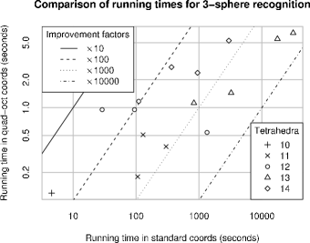
Figure 16: Performance comparisons for 3-sphere recognition

8 Joint Coordinates

We finish this paper with an exploratory discussion of joint coordinates for octagonal almost normal surfaces. Where quadrilateral-octagon coordinates reduce the dimension of the underlying vector space from $10n$ to $6n$, joint coordinates reduce this even further from $6n$ to $3n$. The key idea is to use negative coordinates for octagons and positive coordinates for quadrilaterals, noting from the quadrilateral-octagon constraints that the two cannot occur together within the same tetrahedron.

Joint coordinates have a number of appealing properties. Not only is their dimension small, but they carry the same information as quadrilateral-octagon coordinates (in contrast to the step from standard to quadrilateral-octagon coordinates, where we lose information about vertex links). Moreover, joint coordinates adhere to almost the same constraints in $\mathbb{R}^{3n}$ as Tollefson’s quadrilateral coordinates for normal surfaces—in particular, they satisfy the original quadrilateral matching equations and quadrilateral constraints from Section 2.

There is a cost however, which is the loss of convexity. For joint coordinates, we must allow one coordinate (but no more) to become negative. As a result we no longer work in the non-negative orthant of $\mathbb{R}^{3n}$, but rather the non-negative orthant and the $3n$ “almost non-negative” orthants that border it. This has severe consequences for the enumeration algorithms described in Section 6, which rely on convexity as a core requirement.

Nevertheless, it is pleasing to be able to express octagonal almost normal surfaces using essentially the same coordinate system as normal surfaces, and to do so in a way that portrays them as a natural extension of Tollefson’s original framework (where our extension involves simply stepping “just outside” the non-negative orthant).

The layout of this section is as follows. We begin by describing the way in which we number quadrilateral and octagon types within each tetrahedron, which must be done carefully for joint coordinates to work. Following this, we define joint coordinates and develop the corresponding uniqueness and admissibility results. We then present an example using a one-tetrahedron triangulation, where we show graphically how the vector representations of normal and almost normal surfaces appear in the corresponding solution space in $\mathbb{R}^{3}$. To finish, we discuss how the loss of convexity affects both the projective solution space and the enumeration algorithms.

Definition 8.1 (Quadrilateral and Octagon Numbering)

Let $\Delta$ be any tetrahedron in some compact 3-manifold triangulation. Within $\Delta$, we number the quadrilateral and octagon types $1$, $2$ and $3$ so that, for each $i\in\{1,2,3\}$, the two edges of $\Delta$ that quadrilaterals of type $i$ never meet are the same two edges of $\Delta$ that octagons of type $i$ meet twice. This correspondence between quadrilaterals and octagons is illustrated in Figure 17.

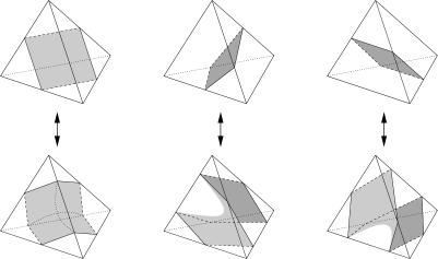
Figure 17: The correspondence between quadrilaterals and octagons

This numbering scheme is very natural, in that the correspondence between quadrilaterals and octagons reflects the natural symmetries of these discs within a tetrahedron. One can also think of an octagon of type $i$ as being obtained from a quadrilateral of type $i$ by pulling each edge of the quadrilateral around and over the nearby vertex of the tetrahedron.

With our numbering scheme in place, we are now ready to define joint coordinates. Since we plan to present joint coordinates as a natural extension of Tollefson’s quadrilateral coordinates, we define them for both normal and almost normal surfaces as follows.

Definition 8.2 (Joint Vector Representation)

Let $\mathcal{T}$ be a compact 3-manifold triangulation formed from the $n$ tetrahedra $\Delta_{1},\ldots,\Delta_{n}$, and let $S$ be an embedded normal or octagonal almost normal surface in $\mathcal{T}$. For each tetrahedron $\Delta_{i}$, let $q_{i,1}$, $q_{i,2}$ and $q_{i,3}$ denote the number of quadrilateral discs of each type, and let $k_{i,1}$, $k_{i,2}$ and $k_{i,3}$ denote the number of octagonal discs of each type in $\Delta_{i}$ contained in the surface $S$.

Then the joint vector representation of $S$, denoted $\mathbf{j}(S)$, is the $3n$-dimensional vector

$$\mathbf{j}(S)~{}=\,(~{} q_{1,1}-k_{1,1},\,q_{1,2}-k_{1,2} ,\,q_{1,3}-k_{1,3}\ ;$$

$$q_{2,1}-k_{2,1},\,q_{2,2}-k_{2,2} ,\,q_{2,3}-k_{2,3}\ ;$$

$$\ldots ,\,q_{n,3}-k_{n,3}\ ).$$

Our first task is to show that joint coordinates in $3n$ dimensions retain all of the information carried by quadrilateral-octagon coordinates in $6n$ dimensions.

Lemma 8.3

Let $\mathcal{T}$ be a compact 3-manifold triangulation, and let $S$ and $S^{\prime}$ be embedded normal or octagonal almost normal surfaces in $\mathcal{T}$. Then the joint vector representations $\mathbf{j}(S)$ and $\mathbf{j}(S^{\prime})$ are equal if and only if the quadrilateral-octagon vector representations $\mathbf{k}(S)$ and $\mathbf{k}(S^{\prime})$ are equal.

Here we define the quadrilateral-octagon vector representation for an embedded normal surface in the obvious way, by setting all octagonal coordinates to zero.

Proof.

It is clear that if $\mathbf{k}(S)=\mathbf{k}(S^{\prime})$ then $\mathbf{j}(S)=\mathbf{j}(S^{\prime})$. Suppose conversely that $\mathbf{j}(S)=\mathbf{j}(S^{\prime})$, and consider the $(i,t)$th coordinate $j_{i,t}=q_{i,t}-k_{i,t}$.

For both $S$ and $S^{\prime}$ we know that $q_{i,t}\geq 0$ and $k_{i,t}\geq 0$. Moreover, since $S$ and $S^{\prime}$ satisfy the quadrilateral-octagon constraints, we know that they can each have $q_{i,t}>0$ or $k_{i,t}>0$ but not both. It follows that for both $S$ and $S^{\prime}$ we have one of the following situations:

• $j_{i,t}=0$, in which case $q_{i,t}=k_{i,t}=0$;

• $j_{i,t}=K>0$, in which case $q_{i,t}=K$ and $k_{i,t}=0$;

• $j_{i,t}=-K<0$, in which case $q_{i,t}=0$ and $k_{i,t}=K$.

That is, we can reconstruct the individual constituents $q_{i,t}$ and $k_{i,t}$ from the joint coordinate $j_{i,t}$, whereupon we obtain $\mathbf{k}(S)=\mathbf{k}(S^{\prime})$. ∎

As an immediate consequence of Lemmas 8.3 and 4.2, we obtain the following uniqueness result for joint vector representations:

Corollary 8.4

Let $\mathcal{T}$ be a compact 3-manifold triangulation, and let $S$ and $S^{\prime}$ be embedded normal or octagonal almost normal surfaces in $\mathcal{T}$. Then the joint vector representations $\mathbf{j}(S)$ and $\mathbf{j}(S^{\prime})$ are equal if and only if either (i) the surfaces $S$ and $S^{\prime}$ are normal isotopic, or (ii) $S$ and $S^{\prime}$ can be made normal isotopic by adding or removing vertex linking components.

We proceed now to give a complete classification of joint vector representations of embedded normal and octagonal almost normal surfaces. As indicated earlier, one of the appealing features of joint coordinates is that this classification corresponds precisely to Tollefson’s theorem for embedded normal surfaces (Theorem 2.6), except for the fact that we must allow one coordinate to become negative.

Theorem 8.5

Let $\mathcal{T}$ be a compact 3-manifold triangulation formed from $n$ tetrahedra. An integer vector $\mathbf{w}\in\mathbb{R}^{3n}$ is the joint vector representation of an embedded normal or octagonal almost normal surface in $\mathcal{T}$ if and only if:

• At most one coordinate of $\mathbf{w}$ is negative;

• $\mathbf{w}$ satisfies the quadrilateral matching equations for $\mathcal{T}$ (Definition 2.4);

• $\mathbf{w}$ satisfies the quadrilateral constraints for $\mathcal{T}$ (Definition 2.5);

• If there is a negative coordinate in $\mathbf{w}$, then this coordinate is set to $-1$.

Moreover, such a vector represents an embedded normal surface in $\mathcal{T}$ if and only if all of its coordinates are non-negative.

It is worth pointing out that we interpret the quadrilateral matching equations and the quadrilateral constraints literally for any $3n$-dimensional vector. We do not try to “reconstruct” quadrilateral coordinates from $\mathbf{w}$, but instead we read Definitions 2.4 and 2.5 precisely as given. In particular, the vector

$$\mathbf{w}~{}=\,\left(\ j_{1,1},j_{1,2},j_{1,3}\ ;\ \ldots,j_{n,3}\ \right)\in\mathbb{R}^{3n}$$

is deemed to satisfy the quadrilateral constraints if at most one of $j_{i,1}$, $j_{i,2}$ and $j_{i,3}$ is non-zero for any given $i$. Likewise, $\mathbf{w}$ satisfies the quadrilateral matching equations if for each non-boundary edge $e$ of $\mathcal{T}$ we have

$$j_{i_{1},u_{1}}+j_{i_{2},u_{2}}+\ldots+j_{i_{t},u_{t}}=j_{i_{1},d_{1}}+j_{i_{2},d_{2}}+\ldots+j_{i_{t},d_{t}},$$

where each $u_{k}$ is the number of an upward quadrilateral type meeting $e$ in the $i_{k}$th tetrahedron of $\mathcal{T}$, and each $d_{k}$ is the number of a downward quadrilateral type meeting $e$ in the $i_{k}$th tetrahedron of $\mathcal{T}$.

Proof.

Normal surfaces (as opposed to almost normal surfaces) are easily dealt with. Suppose that $S$ is some embedded normal surface in $\mathcal{T}$. Then we have $\mathbf{j}(S)=\mathbf{q}(S)$, and it is clear from Theorem 2.6 that $\mathbf{j}(S)$ satisfies the four conditions given in this theorem, and that every coordinate of $\mathbf{j}(S)$ is non-negative. Conversely, suppose that some integer vector $\mathbf{w}\in\mathbb{R}^{3n}$ satisfies these four conditions, and that all of its coordinates are non-negative. Then $\mathbf{w}$ satisfies the conditions of Theorem 2.6, whereupon it follows that $\mathbf{w}$ is the quadrilateral vector representation—and therefore also the joint vector representation—of some embedded normal surface in $\mathcal{T}$.

We turn our attention now to the more interesting case of octagonal almost normal surfaces. The key observation is the following. Consider the quadrilateral-octagon matching equation derived from some non-boundary edge $e$ of the triangulation, as described in Definition 4.3, and let $\Delta$ be some tetrahedron containing $e$. If we use the numbering scheme of Definition 8.1, then the $i$th quadrilateral type in $\Delta$ is an upward quadrilateral if and only if the $i$th octagon type in $\Delta$ is a downward octagon, and vice versa. This is easily verified by examining Figure 9.

Using this observation, we can reduce each quadrilateral-octagon matching equation (4.3) to the following:

$$(q_{i_{1},u_{1}}-k_{i_{1},u_{1}})+\ldots+(q_{i_{1},u_{t}}-k_{i_{1},u_{t}})=(q_{i_{1},d_{1}}-k_{i_{1},d_{1}})+\ldots+(q_{i_{1},d_{t}}-k_{i_{1},d_{t}}),$$ (8.8)

where the coordinates $q_{i_{1},u_{1}},q_{i_{2},u_{2}},\ldots,q_{i_{t},u_{t}}$ and $q_{i_{1},d_{1}},q_{i_{2},d_{2}},\ldots,q_{i_{t},d_{t}}$ correspond to the upward and downward quadrilaterals respectively about the edge $e$. Translated into joint coordinates, this reduces further to

$$j_{i_{1},u_{1}}+\ldots+j_{i_{1},u_{t}}=j_{i_{1},d_{1}}+\ldots+j_{i_{1},d_{t}},$$ (8.9)

which is identical to the corresponding quadrilateral matching equation in $\mathbb{R}^{3n}$.

We can now finish the proof of Theorem 8.5. Suppose that $S$ is some octagonal almost normal surface in $\mathcal{T}$. Then the following observations follow immediately from Theorem 4.5:

• Precisely one octagonal coordinate in $\mathbf{k}(S)$ is non-zero, and the corresponding quadrilateral coordinate in $\mathbf{k}(S)$ must be zero as a result. Therefore precisely one coordinate of $\mathbf{j}(S)$ is negative.

• The quadrilateral-octagon vector representation $\mathbf{k}(S)$ satisfies each quadrilateral-octagon matching equation as described by (8.8). Therefore the joint vector representation $\mathbf{j}(S)$ satisfies each quadrilateral matching equation, as described by (8.9).

• For each tetrahedron of $\mathcal{T}$, at most one of the six corresponding quadrilateral and octagonal coordinates in $\mathbf{k}(S)$ is non-zero, and so at most one of the three corresponding joint coordinates in $\mathbf{j}(S)$ is non-zero. Therefore $\mathbf{j}(S)$ satisfies the quadrilateral constraints.

• The unique non-zero octagonal coordinate in $\mathbf{k}(S)$ has value $+1$, and so the unique negative coordinate in $\mathbf{j}(S)$ has value $-1$.

Therefore the joint vector representation $\mathbf{j}(S)$ satisfies all four conditions listed in the statement of this theorem.

Conversely, suppose that some integer vector

$$\mathbf{w}~{}=\,\left(\ j_{1,1},j_{1,2},j_{1,3}\ ;\ \ldots,j_{n,3}\ \right)\in\mathbb{R}^{3n}$$

satisfies all four conditions listed in this theorem statement, and that one of its coordinates is negative (recalling that the non-negative case was dealt with at the beginning of this proof). We define the $6n$-dimensional vector

$$\mathbf{w}^{\prime}~{}=\,\left(\ q_{1,1},q_{1,2},q_{1,3},\ k_{1,1},k_{1,2},k_{1,3}\ ;\ \ldots,k_{n,3}\ \right)\in\mathbb{R}^{6n}$$

by setting

$$q_{i,t}=\left\{\begin{array}[]{l@{\quad}l}j_{i,t}&\mbox{if $j_{i,t}\geq 0$;}\\ 0&\mbox{if $j_{i,t}<0$,}\end{array}\right.\quad\mbox{and}\quad k_{i,t}=\left\{\begin{array}[]{l@{\quad}l}0&\mbox{if $j_{i,t}\geq 0$;}\\ -j_{i,t}&\mbox{if $j_{i,t}<0$.}\end{array}\right.$$

By using the four conditions of this theorem statement and following the previous argument in reverse, it is simple to show that $\mathbf{w}^{\prime}$ satisfies the conditions of Theorem 4.5. It follows then that $\mathbf{w}^{\prime}$ is the quadrilateral-octagon vector representation of some octagonal almost normal surface in $\mathcal{T}$, and so $\mathbf{w}$ is the joint vector representation of this same surface. ∎

Because joint coordinates are $3n$-dimensional, we are able to visualise them explicitly in $\mathbb{R}^{3}$ for a one-tetrahedron triangulation. We do just this in the following example to illustrate the various conditions of Theorem 8.5.

Example 8.6

Let $\mathcal{S}$ be the following compact 3-manifold triangulation (which we will shortly prove represents the 3-sphere). We begin with the single tetrahedron $\mathit{ABCD}$, and identify faces $\mathit{ABC}\leftrightarrow\mathit{BCD}$ (with a twist) and $\mathit{ABD}\leftrightarrow\mathit{ACD}$ (folded directly over the common edge $\mathit{AD}$), as illustrated in Figure 18. The resulting triangulation has one tetrahedron, one vertex (since $A$, $B$, $C$ and $D$ are all identified), and two edges (where $\mathit{AB}$, $\mathit{BC}$, $\mathit{CD}$, $\mathit{BD}$ and $\mathit{AC}$ are all identified, and $\mathit{AD}$ is left in a class of its own).

Figure 18: The one-tetrahedron triangulation $\mathcal{S}$

Let $\Delta$ represent the sole tetrahedron of $\mathcal{S}$, and number the three quadrilateral types in $\Delta$ so that types 1, 2 and 3 separate the edge pairs ($\mathit{AB},\mathit{CD}$), ($\mathit{AC},\mathit{BD}$) and ($\mathit{AD},\mathit{BC}$) respectively. We find then that both joint matching equations for $\mathcal{S}$ (one for each edge) reduce to the form $j_{1,1}=j_{1,2}$.

We plot the resulting solution space in $\mathbb{R}^{3}$ in Figure 19. In the top-left diagram, we shade the region in which $\mathbf{w}=(j_{1,1},j_{1,2},j_{1,3})\in\mathbb{R}^{3}$ has at most one negative coordinate (for clarity, we restrict our shading to the interior of a sphere around the origin). In the top-right diagram, we shade the intersection of this region with the hyperplane $j_{1,1}=j_{1,2}$, which gives us the closed half-plane $H=\{(x,x,z)\,|\,x\geq 0\}$. If we wish to enforce the quadrilateral constraints then we must restrict our attention to the three coordinate axes (where at most one coordinate is non-zero); the final intersection of $H$ with these three axes is plotted in the bottom-left diagram. The resulting solution space is simply the entire $j_{1,3}$ axis, taken in both directions.

Figure 19: Building the solution space for the triangulation $\mathcal{S}$

From Theorem 8.5 it follows that, if we ignore vertex linking components, then the normal and octagonal normal surfaces in $\mathcal{S}$ correspond precisely to the integer points

$$\{(0,0,k)\,|\,k\in\mathbb{Z},\ k\geq-1\}.$$

With some further investigation we can classify these surfaces as follows:

• $(0,0,0)$ represents the empty surface;

• $(0,0,k)$ for $k\geq 1$ represents $k$ copies of the embedded normal torus surrounding the edge $\mathit{AD}$, which is referred to by Jaco and Rubinstein as a thin edge link [15];

• $(0,0,-1)$ is an octagonal almost normal 2-sphere.

These surfaces are individually plotted in the bottom-right diagram of Figure 19.

To finish, we note that (i) there are no normal 2-spheres (aside from the vertex link which we have ignored), and so $\mathcal{S}$ is a 0-efficient triangulation, and that (ii) $\mathcal{S}$ contains an octagonal almost normal 2-sphere. Using Theorem 5.3 and noting that $\mathcal{S}$ is orientable, it follows that $\mathcal{S}$ is in fact a triangulation of the 3-sphere.

A natural question to ask at this point is what becomes of the projective solution space in joint coordinates. Recall that in other coordinate systems, the non-negative orthant and the matching equations intersect to give a convex polyhedral cone, and that the projective solution space is a cross-section of this cone, taken by intersecting the cone with the hyperplane $\sum x_{i}=1$.

The difficulty we face with joint coordinates is that we no longer have a convex polyhedral cone to work with. Instead we begin with the union of $3n+1$ orthants in $\mathbb{R}^{3n}$ (where at most one coordinate is non-negative), which is not even a convex set. Upon intersecting this with the joint matching equations, we obtain a set $\mathcal{P}$ with the following properties. $\mathcal{P}$ is a cone in the sense that $\mathbf{x}\in\mathcal{P}$ implies that $\lambda\mathbf{x}\in\mathcal{P}$ for any $\lambda\geq 0$, but like the union of orthants before it, $\mathcal{P}$ might not be convex (although in Example 8.6 it happens to be). More importantly, $\mathcal{P}$ can contain diametrically opposite points (such as $(0,0,\pm 1)$ in our example), and so in general we cannot form a cross-section by slicing through $\mathcal{P}$ with a hyperplane.

We could perhaps take a cross-section using the unit sphere, but this would lift us out of the world of polytopes, making it difficult to design algorithms. Perhaps the simplest solution is to take a cross section using the “polyhedral unit sphere” $\sum|x_{i}|=1$, as illustrated in Figure 20. Continuing with Example 8.6, the left-hand diagram of Figure 20 shows the intersection of our four original orthants with the “sphere” $|j_{1,1}|+|j_{1,2}|+|j_{1,3}|=1$, and the right-hand diagram shows the subsequent intersection with the matching equation $j_{1,1}=j_{1,2}$.

Figure 20: Constructing the “projective solution space” in joint coordinates

Although we are now able to define the projective solution space in a sensible way, we do not obtain a single convex polytope as a result. Instead we obtain $3n+1$ distinct convex polytopes—one for each of the original orthants—joined together along their boundaries. To enumerate the vertices of this structure would therefore require $3n+1$ distinct passes through the vertex enumeration algorithm, bringing us back to the scheme of Casson that we discussed in Section 6.3. It is worth noting again that the polytope of this structure that sits within the non-negative orthant is precisely Tollefson’s quadrilateral projective solution space for normal surfaces.

It follows then that joint coordinates do not appear practical for use in enumeration algorithms. Nevertheless, they have appealing geometric properties that may render them useful for other purposes:

• They live in a remarkably small number of dimensions;

• They express the space of admissible vectors for octagonal almost normal surfaces as a natural geometric extension of Tollefson’s space for normal surfaces, obtained simply by expanding our scope from the non-negative orthant to include the neighbouring “almost non-negative” orthants.

As an immediate application, these properties make joint coordinates a useful tool for visualising the almost normal solution space. More generally, they could perhaps open the way for new theoretical insights into the structure of the solution space.

To illustrate the latter point, we can draw analogies with Casson’s edge weight coordinates for normal surfaces, which are developed and exploited in [3]. Like joint coordinates, edge weight coordinates use very few dimensions and are geometrically appealing, but a loss of convexity makes them impractical for use in algorithms. Nevertheless, their tight geometric structure has led to new theoretical and combinatorial insights, and we hope that joint coordinates can offer the same.

Benjamin A. Burton
School of Mathematics and Physics, The University of Queensland
Brisbane QLD 4072, Australia
(bab@debian.org)

References

- [1] Ian Agol, Joel Hass, and William Thurston, 3-manifold knot genus is NP-complete, STOC ’02: Proceedings of the Thiry-Fourth Annual ACM Symposium on Theory of Computing (New York, NY, USA), ACM, 2002, pp. 761–766.
- [2] Benjamin A. Burton, Regina: Normal surface and 3-manifold topology software, http://regina.sourceforge.net/, 1999–2009.
- [3] , Minimal triangulations and normal surfaces, Ph.D. thesis, University of Melbourne, 2003, available from http://regina.sourceforge.net/.
- [4] , Introducing Regina, the 3-manifold topology software, Experiment. Math. 13 (2004), no. 3, 267–272.
- [5] , Optimizing the double description method for normal surface enumeration, To appear in Math. Comp., arXiv:0808.4050, August 2008.
- [6] , Converting between quadrilateral and standard solution sets in normal surface theory, To appear in Algebr. Geom. Topol., arXiv:0901.2629, January 2009.
- [7] , Extreme cases in normal surface enumeration, In preparation, 2009.
- [8] Wolfgang Haken, Theorie der Normalflächen, Acta Math. 105 (1961), 245–375.
- [9] , Über das Homöomorphieproblem der 3-Mannigfaltigkeiten. I, Math. Z. 80 (1962), 89–120.
- [10] Joel Hass, Jeffrey C. Lagarias, and Nicholas Pippenger, The computational complexity of knot and link problems, J. Assoc. Comput. Mach. 46 (1999), no. 2, 185–211.
- [11] Martin V. Hildebrand and Jeffrey R. Weeks, A computer generated census of cusped hyperbolic 3-manifolds, Computers and Mathematics (Cambridge, MA, 1989), Springer, New York, 1989, pp. 53–59.
- [12] Craig D. Hodgson and Jeffrey R. Weeks, Symmetries, isometries and length spectra of closed hyperbolic three-manifolds, Experiment. Math. 3 (1994), no. 4, 261–274.
- [13] William Jaco, David Letscher, and J. Hyam Rubinstein, Algorithms for essential surfaces in 3-manifolds, Topology and Geometry: Commemorating SISTAG, Contemporary Mathematics, no. 314, Amer. Math. Soc., Providence, RI, 2002, pp. 107–124.
- [14] William Jaco and Ulrich Oertel, An algorithm to decide if a -manifold is a Haken manifold, Topology 23 (1984), no. 2, 195–209.
- [15] William Jaco and J. Hyam Rubinstein, 0-efficient triangulations of 3-manifolds, J. Differential Geom. 65 (2003), no. 1, 61–168.
- [16] William Jaco and Jeffrey L. Tollefson, Algorithms for the complete decomposition of a closed -manifold, Illinois J. Math. 39 (1995), no. 3, 358–406.
- [17] Hellmuth Kneser, Geschlossene Flächen in dreidimensionalen Mannigfaltigkeiten, Jahresbericht der Deut. Math. Verein. 38 (1929), 248–260.
- [18] Marc Lackenby, An algorithm to determine the Heegaard genus of simple 3-manifolds with nonempty boundary, Algebr. Geom. Topol. 8 (2008), no. 2, 911–934.
- [19] T. S. Motzkin, H. Raiffa, G. L. Thompson, and R. M. Thrall, The double description method, Contributions to the Theory of Games, Vol. II (H. W. Kuhn and A. W. Tucker, eds.), Annals of Mathematics Studies, no. 28, Princeton University Press, Princeton, NJ, 1953, pp. 51–73.
- [20] J. Hyam Rubinstein, An algorithm to recognize the -sphere, Proceedings of the International Congress of Mathematicians (Zürich, 1994), vol. 1, Birkhäuser, 1995, pp. 601–611.
- [21] , Polyhedral minimal surfaces, Heegaard splittings and decision problems for -dimensional manifolds, Geometric Topology (Athens, GA, 1993), AMS/IP Stud. Adv. Math., vol. 2, Amer. Math. Soc., 1997, pp. 1–20.
- [22] , An algorithm to recognise small Seifert fiber spaces, Turkish J. Math. 28 (2004), no. 1, 75–87.
- [23] Abigail Thompson, Thin position and the recognition problem for , Math. Res. Lett. 1 (1994), no. 5, 613–630.
- [24] William P. Thurston, The geometry and topology of 3-manifolds, Lecture notes, Princeton University, 1978.
- [25] Stephan Tillmann, Normal surfaces in topologically finite 3-manifolds, Enseign. Math. (2) 54 (2008), 329–380.
- [26] Jeffrey L. Tollefson, Normal surface -theory, Pacific J. Math. 183 (1998), no. 2, 359–374.
- [27] Robin Todd Wilson, Meridional almost normal surfaces in knot complements, Algebr. Geom. Topol. 8 (2008), no. 3, 1717–1740.