Aharonov-Bohm oscillations in coupled quantum dots: Effect of electron-electron interactions

Abstract

We theoretically analyze the effect of electron-electron interactions on Aharonov-Bohm (AB) current oscillations in ring-shaped systems with metallic quantum dots pierced by external magnetic field. We demonstrate that electron-electron interactions suppress the amplitude of AB oscillations $I_{AB}$ at all temperatures down to $T=0$ and formulate quantitative predictions which can be verified in future experiments. We argue that the main physical reason for such interaction-induced suppression of $I_{AB}$ is electron dephasing while Coulomb blockade effects remain insignificant in the case of metallic quantum dots considered here. We also emphasize a direct relation between our results and the so-called $P(E)$-theory describing tunneling of interacting electrons.

I Introduction

Aharonov-Bohm (AB) oscillations of conductance as a function of the magnetic flux $\Phi$ piercing the system represent one of the fundamental properties of meso- and nanoscale conductors which is directly related to quantum coherence of electrons ArSh . Coherent electrons propagating along different paths in multiply connected conductors, such as, e.g., metallic rings, can interfere. Such interference effect results in a specific quantum contribution to the system conductance $\delta G$. Threading the ring by an external magnetic flux $\Phi$ one can control the relative phase of the wave functions of interfering electrons, thus changing the magnitude of $\delta G$ as a function of $\Phi$. The dependence $\delta G(\Phi)$ turns out to be periodic with the fundamental period equal to the flux quantum $\Phi_{0}=hc/e$.

It is important to emphasize that the phase of the electron wave function is sensitive to its particular path. In diffusive conductors electrons can propagate along very many different paths, hence picking up different phases. Averaging over these (random) phases or, equivalently, over disorder configurations yields the amplitude of AB oscillations $\delta G(\Phi)$ with the period $\Phi_{0}$ to vanish in diffusive conductors ArSh . There exists, however, a special class of electron trajectories which interference is not sensitive to disorder averaging. These are all pairs of time-reversed paths which are also responsible for the phenomenon of weak localization CS . In multiply connected disordered conductors interference between these trajectories gives rise to non-vanishing AB oscillations with the principle period $\Phi_{0}/2$. Such oscillations will be analyzed below in this paper.

It is well known that various kinds of interactions, such as electron-electron and electron-phonon interactions, electron scattering on magnetic impurities etc. can lead to decoherence of electrons thus reducing their ability to interfere. Accordingly, AB oscillations should be sensitive to all these processes and can be used as a tool to probe the fundamental effect of interactions on quantum coherence of electrons in nanoscale conductors. Recently it was demonstrated GZ06 ; GZ08 ; GZ07 that the effect of quantum decoherence by electron-electron interactions can be conveniently studied employing the model of a system of coupled quantum dots (or scatterers). This model might embrace essentially all types of disordered conductors and allows for a straightforward non-perturbative treatment of electron-electron interactions. It also allows to establish a direct and transparent relation GZ08 ; GZ07 between the problem of quantum decoherence by electron-electron interactions and the so-called $P(E)$ theory SZ ; IN , see also GZ99 for an earlier discussion of this important point. In this paper we employ a similar model in order to study the effect of electron-electron interactions on AB oscillations in disordered nanorings.

The structure of our paper is as follows. In Sec. 2 we define our model and outline our general real time path integral formalism employed in this work. Sec. 3 is devoted to a detailed derivation of the effective action for our problem in terms of fluctuating Hubbard-Stratonovich fields mediating electron-electron interactions. With the aid of this effective action we then evaluate Aharonov-Bohm conductance of the ring in the presence of electron-electron interactions. This task is accomplished in Sec. 4. A brief discussion of our results is presented in Sec. 5. Some technical details of disorder averaging are relegated to Appendices.

II The model and basic formalism

Below we will analyze the system depicted in Fig. 1. The structure consists of two chaotic quantum dots (L and R) characterized by mean level spacing $\delta_{L}$ and $\delta_{R}$. Here we will restrict our attention to the case of metallic quantum dots with $\delta_{L,R}$ being the lowest energy parameters in the problem. These dots are interconnected via two tunnel junctions J₁ and J₂ with conductances $G_{t1}$ and $G_{t2}$ forming a ring-shaped configuration as shown in Fig. 1. The left and right dots are also connected to the leads (LL and RL) respectively via the barriers J_L and J_R with conductances $G_{L}$ and $G_{R}$. We also define the corresponding dimensionless conductances of all four barriers as $g_{t1,2}=G_{t1,2}R_{q}$ and $g_{L,R}=G_{t1,2}R_{q}$, where $R_{q}=2\pi/e^{2}$ is the quantum resistance unit. These dimensionless conductances are related to the barrier channel transmissions $T_{k}$ via the standard formula $g=2\sum_{k}T_{k}$, where the sum is taken over all conducting channels in the corresponding barrier and an extra factor 2 accounts for the electron spin.

For the sake of convenience in what follows we will assume that dimensionless conductances $g_{L,R}$ are much larger than unity, while the conductances $g_{t1}$ and $g_{t2}$ are small as compared to those of the outer barriers, i.e.

$$g_{L},g_{R}\gg 1,g_{t1},g_{t2}.$$ (1)

The whole structure is pierced by the magnetic flux $\Phi$ through the hole between two central barriers in such way that electrons passing from left to right through different junctions acquire different geometric phases. Applying a voltage across the system one induces the current which shows AB oscillations with changing the external flux $\Phi$.

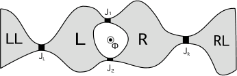
Figure 1: The ring-shaped quantum dot structure under consideration.

The system depicted in Fig. 1 is described by the effective Hamiltonian:

$$\hat{H} = \sum_{i,j=L,R}\frac{C_{ij}\hat{\bm{V}}_{i}\hat{\bm{V}}_{j}}{2}+\hat{\bm{H}}_{LL}+\hat{\bm{H}}_{RL}$$ (2)

$$+\sum_{j=L,R}\hat{\bm{H}}_{j}+\hat{\bm{T}}_{L}+\hat{\bm{T}}_{R}+\hat{\bm{T}},$$

where $C_{ij}$ is the capacitance matrix, $\hat{\bm{V}}_{L(R)}$ is the electric potential operator on the left (right) quantum dot,

$$\hat{\bm{H}}_{LL}=\sum\limits_{\alpha=\uparrow,\downarrow}\int\limits_{LL}d^{3}{\bm{r}}\hat{\Psi}^{\dagger}_{\alpha,LL}({\bm{r}})(\hat{H}_{LL}-eV_{LL})\hat{\Psi}_{\alpha,LL}({\bm{r}}),$$

$$\hat{\bm{H}}_{RL}=\sum\limits_{\alpha=\uparrow,\downarrow}\int\limits_{RL}d^{3}{\bm{r}}\hat{\Psi}^{\dagger}_{\alpha,RL}({\bm{r}})(\hat{H}_{RL}-eV_{RL})\hat{\Psi}_{\alpha,RL}({\bm{r}})$$

are the Hamiltonians of the left and right leads, $V_{LL,RL}$ are the electric potentials of the leads fixed by the external voltage source,

$$\hat{\bm{H}}_{j}=\sum\limits_{\alpha=\uparrow,\downarrow}\int\limits_{j}d^{3}{\bm{r}}\hat{\Psi}^{\dagger}_{\alpha,j}({\bm{r}})(\hat{H}_{j}-e\hat{\bm{V}}_{j})\hat{\Psi}_{\alpha,j}({\bm{r}})$$

defines the Hamiltonians of the left ($j=L$) and right ($j=R$) quantum dots and

$$\hat{H}_{j}=\frac{(\hat{p}_{\mu}-\frac{e}{c}A_{\mu}(r))^{2}}{2m}-\mu+U_{j}(r)$$

is the one-particle Hamiltonian of electron in $j$-th quantum dot with disorder potential $U_{j}(r)$. Electron transfer between the left and the right quantum dots will be described by the Hamiltonian

$$\hat{\bm{T}}=\sum_{\alpha=\uparrow,\downarrow}\int_{J_{1}+J_{2}}d^{2}{\bm{r}}\,\big{[}t({\bm{r}})\hat{\Psi}^{\dagger}_{\alpha,L}({\bm{r}})\hat{\Psi}_{\alpha,R}({\bm{r}})+{\rm c.c.}\big{]}.$$

Here the integration runs over the total area of both tunnel barriers J₁ and J₂. The Hamiltonian $\hat{\bm{T}}_{L(R)}$ describing electron transfer between the left dot and the left lead (the right dot and the right lead) is defined analogously and are omitted here.

Before we proceed with our analysis the following two remarks are in order. Firstly, we point out that within our approach the effect of electron-electron interactions is accounted for by the voltage operators $\hat{\bm{V}}_{L,R}$ in the effective Hamiltonian (2). In order to avoid misunderstandings we would like to emphasize that this approach is fully equivalent to one employing the usual Coulomb interaction term in the initial Hamiltonian of the system. The operators $\hat{\bm{V}}_{L,R}$ corresponding to fluctuating potentials of the left and right dots emerge as a result of the exact Hubbard-Stratonovich decoupling of the Coulomb term containing the product of four electron operators. This is a standard procedure (described in details, e.g., in Ref. SZ, and elsewhere) which is bypassed here for the sake of brevity.

Secondly, we note that in Ref. GZ06, we have studied weak localization effects in a system of coupled quantum dots within the framework of the scattering matrix formalism combined with the non-linear $\sigma$-model. However, in order to incorporate interaction effects into our consideration – similarly to Refs. GZ08, ; GZ07, – it will be convenient for us to describe inter-dot electron transfer within the tunneling Hamiltonian approach, as specified above. For clarity let us briefly recapitulate the relation between these two approaches. For this purpose we define the matrix elements $t_{lm}=\langle l|\hat{T}|m\rangle$ between the $l-$th wave function in the left dot and $m-$th wave function in the right dot. Electron transfer between these dots can then be described by a set of eigenvalues of this matrix $\tilde{t}_{k}$ where, as above, the index $k$ labels the conducting channels. These eigenvalues are related to the barrier channel transmissions $T_{k}$ as B

$$T_{k}=\frac{4\pi^{2}|\tilde{t}_{k}|^{2}/\delta_{L}\delta_{R}}{(1+\pi^{2}|\tilde{t}_{k}|^{2}/\delta_{L}\delta_{R})^{2}}.$$ (3)

This equation allows to keep track of the relation between two approaches at every stage of our calculation.

We now proceed employing the path integral Keldysh technique. The time evolution of the density matrix of our system is described by the standard equation

$$\hat{\rho}(t)=e^{-i\hat{H}t}\hat{\rho}_{0}\,e^{i\hat{H}t},$$ (4)

where $\hat{H}$ is given by Eq. (2). Let us express the operators $e^{-i\hat{H}t}$ and $e^{i\hat{H}t}$ via path integrals over the fluctuating electric potentials $V_{j}^{F,B}$ defined respectively on the forward and backward parts of the Keldysh contour:

$$e^{-i\hat{H}t} = \int DV_{j}^{F}\;{\rm T}\,\exp\left\{-i\int_{0}^{t}dt^{\prime}\hat{H}\left[V_{j}^{F}(t^{\prime})\right]\right\},$$

$$e^{i\hat{H}t} = \int DV_{j}^{B}\;\tilde{\rm T}\,\exp\left\{i\int_{0}^{t}dt^{\prime}\hat{H}\left[V_{j}^{B}(t^{\prime})\right]\right\}.$$ (5)

Here ${\rm T}\,\exp$ ($\tilde{\rm T}\,\exp$) stands for the time ordered (anti-ordered) exponent and the Hamiltonians $\hat{H}\left[V_{j}^{F}(t^{\prime})\right]$, $\hat{H}\left[V_{j}^{B}(t^{\prime})\right]$ are obtained from the original Hamiltonian (2) if one replaces the operators ${\bf\hat{V}}_{j}(t)$ respectively by the fluctuating voltages $V^{F}_{j}(t^{\prime})$ and $V^{B}_{j}(t^{\prime})$.

Let us define the effective action of our system

$$iS[V^{F},V^{B}] = \ln\left({\rm tr}\left[{\rm T}\,\exp\left\{-i\int_{0}^{t}dt^{\prime}\hat{H}\left[V_{j}^{F}(t^{\prime})\right]\right\}\right.\right.$$ (6)

$$\times\,\left.\left.\hat{\rho}_{0}\tilde{\rm T}\,\exp\left\{i\int_{0}^{t}dt^{\prime}\hat{H}\left[V_{j}^{B}(t^{\prime})\right]\right\}\right]\right).$$

Since the operators $\hat{H}\left[V_{j}^{F}(t^{\prime})\right]$, $\hat{H}\left[V_{j}^{B}(t^{\prime})\right]$ are quadratic in the electron creation and annihilation operators, it is possible to integrate out the fermionic variables and to rewrite the action in the form

$$iS=iS_{C}+iS_{ext}+2\bf Tr\ln\left[\check{G}^{-1}\right].$$ (7)

Here $S_{C}$ is the standard term describing charging effects, $S_{ext}$ accounts for an external circuit and ${\bf\check{G}^{-1}}$ is the inverse Green-Keldysh function of electrons, moving in fluctuating voltages field. It has the following matrix structure:

$${\bf\check{G}^{-1}}=\left(\begin{array}[]{cccc}\hat{G}^{-1}_{LL}&\hat{T}_{L}&0&0\\ \hat{T}^{\dagger}_{L}&\hat{G}^{-1}_{L}&\hat{T}&0\\ 0&\hat{T}^{\dagger}&\hat{G}^{-1}_{R}&\hat{T}_{R}\\ 0&0&\hat{T}^{\dagger}_{R}&\hat{G}^{-1}_{RL}\end{array}\right).$$ (8)

Here each quantum dot as well as two leads is represented by the 2x2 matrix in the Keldysh space:

$$\hat{G}^{-1}_{i}=\left(\begin{array}[]{cc}i\partial_{t}-\hat{H}_{i}+eV^{F}_{i}&0\\ 0&-i\partial_{t}+\hat{H}_{i}-eV^{B}_{i}\end{array}\right)$$ (9)

Tunneling blocks has the following structure in Keldysh space:

$$\hat{T}_{L,R}=\left(\begin{array}[]{cc}-\int\limits_{J_{L,R}}t_{L,R}(r^{\prime})\delta(r^{\prime}-r)dr^{\prime}\qquad\qquad 0\\ \qquad\qquad 0\qquad\qquad\int\limits_{J_{L,R}}t_{L,R}(r^{\prime})\delta(r^{\prime}-r)dr^{\prime}\end{array}\right),$$ (10)

$$\hat{T}=\left(\begin{array}[]{cc}-\int\limits_{J_{1}+J_{2}}t(r^{\prime})\delta(r^{\prime}-r)dr^{\prime}\qquad\qquad 0\\ \qquad\qquad 0\qquad\qquad\int\limits_{J_{1}+J_{2}}t(r^{\prime})\delta(r^{\prime}-r)dr^{\prime}\end{array}\right).$$ (11)

III Effective action

In what follows it will be convenient for us to remove the fluctuating voltage variables and the vector potential from the bare Green functions. This is achieved by performing a unitary transformation under the trace in Eq. (7). As a result we find

$$\hat{T}=\hat{T}_{1}e^{-i\varphi_{g}^{(1)}}+\hat{T}_{2}e^{-i\varphi_{g}^{(2)}}$$ (12)

$$\hat{T}_{l}=\left(\begin{array}[]{c}-e^{i\varphi_{F}}\int\limits_{J_{l}}t(r^{\prime})\delta(r^{\prime}-r)dr^{\prime}\qquad\qquad 0\\ \qquad\qquad 0\qquad\qquad e^{i\varphi_{B}}\int\limits_{J_{l}}t(r^{\prime})\delta(r^{\prime}-r)dr^{\prime}\end{array}\right).$$ (13)

Here we introduced the fluctuating phase differences

$$\varphi_{F,B}(t)=e\int^{t}d\tau(V^{F,B}_{R}(\tau)-V^{F,B}_{L}(\tau))$$ (14)

defined on the forward and backward parts of the Keldysh contour as well as the geometric phases

$$\varphi_{g}^{(1,2)}=\frac{e}{c}\int\limits_{L}^{R}dx_{\mu}A_{\mu}(x),$$ (15)

where the integration contour starts in the left dot, crosses the first ($\varphi_{g}^{(1)}$) or the second ($\varphi_{g}^{(2)}$) junction and ends in the right dot. The difference between these two geometric phases equals to

$$\varphi_{g}^{(1)}-\varphi_{g}^{(2)}=2\pi\Phi/\Phi_{0},$$ (16)

where $\Phi$ is the magnetic flux threading our system.

Let us now expand the exact action $iS$ (7) in powers of $\hat{T}$. Keeping the terms up to the fourth order in the tunneling amplitude, we obtain

$$iS\approx iS_{C}+iS_{ext}+iS_{L}+iS_{R}-2{\bf tr}\left[\hat{G}_{L}\hat{T}\hat{G}_{R}\hat{T}^{\dagger}\right]-$$

$$-{\bf tr}\left[\hat{G}_{L}\hat{T}\hat{G}_{R}\hat{T}^{\dagger}\hat{G}_{L}\hat{T}\hat{G}_{R}\hat{T}^{\dagger}\right]+...$$ (17)

The terms $iS_{L,R}$ define the contributions of the isolated dots (which are of no interest for us here), the second order terms $\propto t^{2}$ yield the well known Ambegaokar-Eckern-Schön (AES) action SZ $iS^{AES}$, and the fourth order terms $\propto t^{4}$ account for the weak localization correction to the system conductance GZ08 ; GZ07 .

Let us first analyze the AES action. Performing averaging of this action over disorder in each dot separately as well as averaging of tunneling amplitudes with the correlation function

$$\overline{t({\bf x})t({\bf y})}=\frac{g_{t}({\bf x})}{8\pi^{2}N_{L}N_{R}}\delta({\bf x}-{\bf y})$$ (18)

we arrive at the following result

$$iS^{AES}=-\int dt_{1}dt_{2}\int\limits_{J_{1}+J_{2}}d{\bf x}\frac{g_{t}({\bf x})}{4\pi^{2}N_{L}N_{R}}\sum\limits_{i,j=F,B}\hat{G}_{L}^{ij}({\bf x}t_{1};{\bf x}t_{2})(-1)^{j}e^{i\varphi_{j}(t_{2})}\hat{G}_{R}^{ji}({\bf x}t_{2};{\bf x}t_{1})(-1)^{i}e^{-i\varphi_{i}(t_{1})},$$ (19)

where the convention $(-1)^{F}=-1,\ (-1)^{B}=1$ is implied. This AES contribution to the action is described by the standard diagram depicted in Fig. 2a. We observe that after disorder averaging the AES action (19) becomes totally independent of the magnetic flux. Hence, this part of the action does not account for the AB effect investigated here.

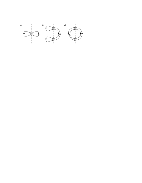
Figure 2: Diagrammatic representation of different contributions originating from expansion of the effective action in powers of the central barrier transmissions: second order (AES) terms (a) and different fourth order terms (b,c).

In order to evaluate the contribution sensitive to the magnetic flux $\Phi$ it is necessary to analyze the last term in Eq. (17). Averaging over realizations of transmission amplitudes yields two types of terms illustrated by the diagrams in Fig. 2b,c. It is straightforward to check that only the contribution generated by the diagram (c) depends on the external magnetic flux, while the diagram (b) does not depend on $\Phi$. On top of that, the terms originating from the diagram (b) turn out to be parametrically small for metallic quantum dots considered here. This observation will be justified in Appendix A.

It follows from the above arguments that only the diagram in Fig. 2c is responsible for the AB effect in our system. Its contribution to the action reads

$$iS_{\Phi}=-\sum\limits_{m,n=1,2}e^{2i(\varphi_{g}^{(n)}-\varphi_{g}^{(m)})}\int dt_{1}dt_{2}dt_{3}dt_{4}\int\limits_{J_{n}}d{\bf x}\int\limits_{J_{m}}d{\bf y}\frac{g_{t}({\bf x})g_{t}({\bf y})}{64\pi^{4}N_{L}^{2}N_{R}^{2}}\times\qquad\quad$$

$$\times\sum\limits_{i,j,k,l=F,B}\hat{G}_{L}^{ij}({\bf x}t_{1};{\bf y}t_{2})(-1)^{j}e^{i\varphi_{j}(t_{2})}\hat{G}_{R}^{jk}({\bf y}t_{2};{\bf x}t_{3})(-1)^{k}e^{-i\varphi_{k}(t_{3})}\times$$

$$\times\hat{G}_{L}^{kl}({\bf x}t_{3};{\bf y}t_{4})(-1)^{l}e^{i\varphi_{l}(t_{4})}\hat{G}_{R}^{li}({\bf y}t_{4};{\bf x}t_{1})(-1)^{i}e^{-i\varphi_{i}(t_{1})}.$$ (20)

Since $\hat{G}_{L,R}$ are the equilibrium Green-Keldysh functions of the dots they can be expressed via retarded ($G^{R}$) and advanced ($G^{A}$) Green functions in the standard manner:

$$\hat{G}_{L,R}({\bf x_{1}}t_{1};{\bf x_{2}}t_{2})=\int dt(G^{R}_{L,R}({\bf x_{1}}t_{1};{\bf x_{2}}t)\hat{F}_{1}(t-t_{2})-\hat{F}_{2}(t_{1}-t)G^{A}_{L,R}({\bf x_{1}}t;{\bf x_{2}}t_{2})),$$ (21)

where

$$\hat{F}_{1}(t)=\left(\begin{array}[]{cc}h(t)&-f(t)\\ h(t)&-f(t)\end{array}\right),\qquad\qquad\hat{F}_{2}(t)=\left(\begin{array}[]{cc}-f(t)&-f(t)\\ h(t)&h(t)\end{array}\right).$$ (22)

Here $f(t)=\int f(E)dE/2\pi$ is the Fourier transform of the Fermi function $f(E)=(\exp(E/T)+1)^{-1}$ and $h(t)=\delta(t)-f(t)$.

What remains is to combine Eqs. (21) and (20) and to average the latter over disorder. This procedure amounts to evaluating the averages of the products of retarded and advanced Green functions in each dot separately. Such averaging can be conveniently accomplished either by means of the diagram technique or with the aid of the non-linear $\sigma$-model. The corresponding calculation is presented in Appendix A. It yields ($i=L,R$):

$$\langle G_{i}^{R}({\bf x_{1}}t_{1};{\bf x_{2}}t_{2})G_{i}^{R}({\bf x_{3}}t_{3};{\bf x_{4}}t_{4})\rangle_{d}=\langle G_{i}^{R}({\bf x_{1}}t_{1};{\bf x_{2}}t_{2})\rangle_{d}\langle G_{i}^{R}({\bf x_{3}}t_{3};{\bf x_{4}}t_{4})\rangle_{d},$$ (23)

$$\langle G_{i}^{A}({\bf x_{1}}t_{1};{\bf x_{2}}t_{2})G_{i}^{A}({\bf x_{3}}t_{3};{\bf x_{4}}t_{4})\rangle_{d}=\langle G_{i}^{A}({\bf x_{1}}t_{1};{\bf x_{2}}t_{2})\rangle_{d}\langle G_{i}^{A}({\bf x_{3}}t_{3};{\bf x_{4}}t_{4})\rangle_{d},$$ (24)

$$\langle G_{i}^{R}({\bf x_{1}}t_{1};{\bf x_{2}}t_{2})G_{i}^{A}({\bf x_{3}}t_{3};{\bf x_{4}}t_{4})\rangle_{d}=\langle G_{i}^{R}({\bf x_{1}}t_{1};{\bf x_{2}}t_{2})\rangle_{d}\langle G_{i}^{A}({\bf x_{3}}t_{3};{\bf x_{4}}t_{4})\rangle_{d}+$$

$$+2\pi N_{i}\varpi(|{\bf x_{1}}-{\bf x_{4}}|)\varpi(|{\bf x_{2}}-{\bf x_{3}}|)\times\qquad\qquad$$

$$\times\mathcal{D}_{i}\left(t_{1}-t_{2};\frac{{\bf x_{1}}+{\bf x_{4}}}{2},\frac{{\bf x_{2}}+{\bf x_{3}}}{2}\right)\delta(t_{1}-t_{2}+t_{3}-t_{4})+$$

$$+2\pi N_{i}\varpi(|{\bf x_{1}}-{\bf x_{3}}|)\varpi(|{\bf x_{2}}-{\bf x_{4}}|)\times\qquad\qquad$$

$$\times\mathcal{C}_{i}\left(t_{1}-t_{2};\frac{{\bf x_{1}}+{\bf x_{3}}}{2},\frac{{\bf x_{2}}+{\bf x_{4}}}{2}\right)\delta(t_{1}-t_{2}+t_{3}-t_{4}),$$ (25)

where $\mathcal{D}_{L,R}(t;{\bf x},{\bf y})$ and $\mathcal{C}_{L,R}(t;{\bf x},{\bf y})$ the diffusons and the Cooperons in the left and right dots and $\varpi(r)=e^{-r/2l}\sin k_{F}r/k_{F}r$. Substituting these averages into the action (20) it is straightforward to observe that only the terms containing the product of two Cooperons yield the contribution which depends on the magnetic flux $\Phi$. This part of the action takes the form

$$iS^{WL}_{\Phi}=-i\sum\limits_{m,n=1,2}e^{2i(\varphi_{g}^{(n)}-\varphi_{g}^{(m)})}\int d\tau_{1}d\tau_{2}\int dt_{1}dt_{2}dt_{3}dt_{4}\int\limits_{J_{n}}d{\bf x}\int\limits_{J_{m}}d{\bf y}\frac{g_{t}({\bf x})g_{t}({\bf y})}{4\pi^{2}N_{L}N_{R}}\times$$

$$\times\mathcal{C}_{L}(\tau_{1};{\bf y},{\bf x})\mathcal{C}_{R}(\tau_{2};{\bf x},{\bf y})e^{i(\varphi^{+}(t_{2})-\varphi^{+}(t_{3})+\varphi^{+}(t_{4})-\varphi^{+}(t_{1}))}\sin\frac{\varphi^{-}(t_{1})}{2}\times$$

$$\times\left[h(t_{1}-t_{2}-\tau_{1})e^{i\frac{\varphi^{-}(t_{2})}{2}}+f(t_{1}-t_{2}-\tau_{1})e^{-i\frac{\varphi^{-}(t_{2})}{2}}\right]\times$$

$$\times\left[h(t_{2}-t_{3}-\tau_{2})e^{-i\frac{\varphi^{-}(t_{3})}{2}}f(t_{3}-t_{4}+\tau_{1})-\right.\quad\qquad\qquad$$

$$\left.-f(t_{2}-t_{3}-\tau_{2})e^{i\frac{\varphi^{-}(t_{3})}{2}}h(t_{3}-t_{4}+\tau_{1})\right]\times$$

$$\times\left[e^{i\frac{\varphi^{-}(t_{4})}{2}}f(t_{4}-t_{1}+\tau_{2})+e^{-i\frac{\varphi^{-}(t_{4})}{2}}h(t_{4}-t_{1}+\tau_{2})\right]+$$

$$+\{L\leftrightarrow R,\varphi^{\pm}\rightarrow-\varphi^{\pm}\},$$ (26)

where we defined the “classical” and the “quantum” components of the fluctuating phase:

$$\varphi^{+}(t)=\frac{\varphi_{F}(t)+\varphi_{B}(t)}{2},\qquad\varphi^{-}(t)=\varphi_{F}(t)-\varphi_{B}(t).$$ (27)

The above expression for the action $S^{WL}_{\Phi}$ (26) fully accounts for coherent oscillations of the system conductance in the lowest non-vanishing order in tunneling. It is important to emphasize that no additional approximations were employed during its derivation and, in particular, the fluctuating phases are exactly accounted for. We will make use of this fact in the next section while considering the effect of electron-electron interactions on AB oscillations in the system under consideration.

IV Current oscillations

Let us now evaluate the current $I$ through our system. For this purpose we will employ a general formula

$$I=-e\int\mathcal{D}^{2}\varphi^{\pm}\frac{\delta S[\varphi^{+},\varphi^{-}]}{\delta\varphi^{-}(t)}e^{iS[\varphi^{+},\varphi^{-}]}.$$ (28)

Substituting the total effective action into this formula we arrive at the result for the current which can be split into two terms $I=I_{0}+\delta I$, where $I_{0}$ is the flux-independent contribution and $\delta I$ is the quantum correction to the current sensitive to the magnetic flux $\Phi$. This correction is determined by the action $iS^{WL}_{\Phi}$, i.e.

$$\delta I=-e\int\mathcal{D}^{2}\varphi^{\pm}\frac{\delta S^{WL}_{\Phi}[\varphi^{+},\varphi^{-}]}{\delta\varphi^{-}(t)}e^{iS[\varphi^{+},\varphi^{-}]}.$$ (29)

Below we will only be interested in finding the quantum correction (29).

In order to evaluate the path integral over the phases $\varphi^{\pm}$ in (29) we note that the contributions $S_{C}$ and $S_{\rm ext}$ in Eq. (17) are quadratic in the fluctuating phases provided our external circuit consists of linear elements. Other contributions to the action are, strictly speaking, non-Gaussian. However, in the interesting for us here metallic limit (1) phase fluctuations can be considered small down to exponentially low energies PZ91 ; Naz99 in which case it suffices to expand both contributions up to the second order $\varphi^{\pm}$. Moreover, this Gaussian approximation becomes exact GGZ05 in the limit of fully open left and right barriers with $g_{L,R}\gg 1$. Thus, in the metallic limit (1) the integral (29) remains Gaussian at all relevant energies and can easily be performed.

This task can be accomplished with the aid of the following correlation functions

$$\langle\varphi^{+}(t)\rangle=eVt,\qquad\langle\varphi^{-}(t)\rangle=0,$$ (30)

$$\langle(\varphi^{+}(t)-\varphi^{+}(0))\varphi^{+}(0)\rangle=-F(t),$$ (31)

$$\langle\varphi^{+}(t)\varphi^{-}(0)+\varphi^{-}(t)\varphi^{+}(0)\rangle=2iK(|t|),$$ (32)

$$\langle\varphi^{+}(t)\varphi^{-}(0)-\varphi^{-}(t)\varphi^{+}(0)\rangle=2iK(t),$$ (33)

$$\langle\varphi^{-}(t)\varphi^{-}(0)\rangle=0,$$ (34)

where the last relation follows directly from the causality principle GZ98 . Here and below we define $V=V_{RL}-V_{LL}$ to be the transport voltage across our system.

Substituting the AB action (26) into Eq. (29) one arrives at the expression containing six different phase averages listed in Appendix B. All these averages in Eqs. (63)-(68) are expressed in terms of two real correlation functions $F(t)=\langle(\hat{\varphi}(t)-\hat{\varphi}(0))^{2}\rangle/2$ and $K(t)=i\langle[\hat{\varphi}(0),\hat{\varphi}(t)]\rangle/2$ defined above in Eqs. (31) and (32). Note that these correlation functions are well familiar from the so-called $P(E)$-theorySZ ; IN describing electron tunneling in the presence of an external environment which can also mimic electron-electron interactions in metallic conductors. They are expressed in terms of an effective impedance $Z(\omega)$ “seen” by the central barriers J₁ and J₂

$$F(t)=e^{2}\int\frac{d\omega}{2\pi}\coth\frac{\omega}{2T}\Re[Z(\omega)]\frac{1-\cos(\omega t)}{\omega},$$ (35)

$$K(t)=e^{2}\int\frac{d\omega}{2\pi}\Re[Z(\omega)]\frac{\sin(\omega t)}{\omega}.$$ (36)

Further evaluation of these correlation functions for our system is straightforward and yields

$$F(t)\simeq\frac{4}{g}\left(\ln\left|\frac{\sinh(\pi Tt)}{\pi T\tau_{RC}}\right|+\gamma\right),$$ (37)

$$K(t)\simeq\frac{2\pi}{g}{\rm sign}(t),$$ (38)

where we defined $g=4\pi/e^{2}Z(0)$ and $\gamma\simeq 0.577$ is the Euler constant. Neglecting the contribution of external leads (which can be trivially restored if needed) and making use of the inequality (1) we obtain $g\simeq 2g_{L}g_{R}/(g_{L}+g_{R})$.

We observe that while $F(t)$ grows with time at any temperature including $T=0$, the function $K(t)$ always remains small in the limit $g\gg 1$ considered here. As we demonstrate in Appendix B, the correlation function $F(t)$ should be fully kept in the exponent in Eqs. (63)-(68) while the correlator $K(t)$ can be safely ignored in the leading order in $1/g$. Then combining all terms we observe that the Fermi function $f(E)$ – though present in the effective action (26) – drops out from the final expression for the quantum correction to the current which takes the form:

$$\delta I(\Phi)=-\sum\limits_{m,n=L,R}\frac{e^{2}Ve^{2i(\varphi_{g}^{(n)}-\varphi_{g}^{(m)})}}{8\pi^{3}N_{L}N_{R}}\int d\tau_{1}d\tau_{2}\int\limits_{J_{n}}d{\bf x}\int\limits_{J_{m}}d{\bf y}g_{t}({\bf x})g_{t}({\bf y})\times$$

$$\times\mathcal{C}_{L}(\tau_{1};{\bf y},{\bf x})\mathcal{C}_{R}(\tau_{2};{\bf x},{\bf y})e^{-2F(\tau_{1})-2F(\tau_{2})+F(\tau_{1}-\tau_{2})+F(\tau_{1}+\tau_{2})}.$$ (39)

We observe that the amplitude of AB oscillations is affected by the electron-electron interaction only via the correlation functions for the “classical” component of the Hubbard-Stratonovich phase $\varphi^{+}$. Both the correlators containing the “quantum” phase $\varphi^{-}$ and the Fermi function $f(E)$ enter only in the next order in $1/g$ which defines weak Coulomb correction to $\delta I$ ignored here. For more details on this point we refer the reader to Refs. GZ08, ; GZ07, .

The result (39) can also be rewritten as

$$\delta I(\Phi)=-I_{AB}(\Phi)-I_{WL1}-I_{WL2},$$ (40)

where the first – flux dependent – term in the right-hand side explicitly accounts for AB oscillations and reads

$$I_{AB}(\Phi)=I_{AB}\cos(4\pi\Phi/\Phi_{0}),$$ (41)

while the last two terms $I_{WL1,2}$ represent the remaining part of the quantum correction to the current which does not depend on $\Phi$.

Already at this stage we would like to clarify the relation between our present results for AB oscillations and those for WL correction to conductance GZ08 . In order to derive Eq. (39) we have evaluated the contributions of all processes illustrated by the diagrams in Fig. 2b,c and identified terms sensitive to the magnetic field which were not considered in Ref. GZ08, . In this way we have obtained the AB current $I_{AB}(\Phi)$ in Eqs. (40), (41) which represents our new result to be analyzed below. The two remaining terms in Eq. (40) are the WL corrections already evaluated in Ref. GZ08, . Towards the end of this section we will explicitly specify the relation between all three contributions to the quantum correction (40).

Let us evaluate the amplitude of AB oscillations $I_{AB}$ for the system with two identical quantum dots with volume $\mathcal{V}$, dwell time $\tau_{D}$ and dimensionless conductances $g_{L}=g_{R}\equiv g=4\pi/\delta\tau_{D}$, where $\delta=1/\mathcal{V}N$ is the dot mean level spacing and $N$ is the electron density of states. In this case the Cooperons take the form

$$\mathcal{C}_{L}(t;{\bf x},{\bf y})=\mathcal{C}_{R}(t;{\bf x},{\bf y})=\frac{\theta(t)}{\mathcal{V}}e^{-t/\tau_{D}}.$$ (42)

Defining dimensionless conductances of central barriers as $g_{t1,2}=\int_{J_{1,2}}g_{t}(x)dx$ we obtain

$$I_{AB}=\frac{e^{2}g_{t1}g_{t2}\delta^{2}V}{4\pi^{3}}\int\limits_{0}^{\infty}d\tau_{1}d\tau_{2}e^{-\frac{\tau_{1}+\tau_{2}}{\tau_{D}}-2F(\tau_{1})-2F(\tau_{2})+F(\tau_{1}-\tau_{2})+F(\tau_{1}+\tau_{2})}.$$ (43)

In the absence of electron-electron interactions ($F(\tau)\to 0$) this formula yields:

$$I_{AB}^{(0)}=\frac{4e^{2}g_{t1}g_{t2}V}{\pi g^{2}}.$$ (44)

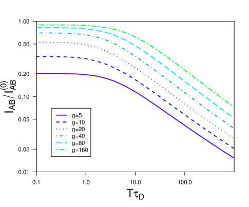
Figure 3: (Color online) The ratio $I_{AB}/I_{AB}^{(0)}$ versus temperature at different values of dimensionless conductance $g$.

In order to account for the effect of interactions we need to specify the effective impedance $Z(\omega)$. Its real part takes the form

$$\Re Z(\omega)=\frac{4\pi}{e^{2}g}\left(\frac{\tau^{2}}{\tau^{2}_{RC}}\frac{1}{\omega^{2}\tau^{2}+1}+\frac{\pi\delta(\omega)}{\tau_{D}+\tau_{RC}}\right),$$ (45)

where $1/\tau=1/\tau_{D}+1/\tau_{RC}$, $\tau_{RC}=\pi/gE_{C}$ is the $RC$-time and $E_{C}$ is an effective charging energy of our system. Eq. (43) demonstrates that electron-electron interactions always tend to suppress the amplitude of AB oscillations $I_{AB}$ below its non-interacting value (44). Combining Eqs. (37) and (45) with (43) at high enough temperatures we obtain

$$\frac{I_{AB}}{I_{AB}^{(0)}}=\left\{\begin{array}[]{lc}e^{-\frac{8\gamma}{g}}\frac{(2\pi T\tau_{RC})^{8/g}}{1+4\pi T\tau_{D}/g},&\tau_{D}^{-1}\lesssim T\lesssim\tau_{RC}^{-1},\\ \frac{1}{2\tau_{D}}\left(\frac{g\tau_{RC}}{T}\right)^{1/2},&\tau_{RC}^{-1}\lesssim T,\end{array}\right.$$ (46)

while in the low temperature limit we find

$$\frac{I_{AB}}{I_{AB}^{(0)}}=e^{-\frac{8\gamma}{g}}\left(\frac{2\tau_{RC}}{\tau_{D}}\right)^{8/g},\qquad T\lesssim\tau_{D}^{-1}.$$ (47)

The latter result demonstrates that interaction-induced suppression of AB oscillations in metallic dots with $\tau_{RC}\ll\tau_{D}$ persists down to $T=0$.

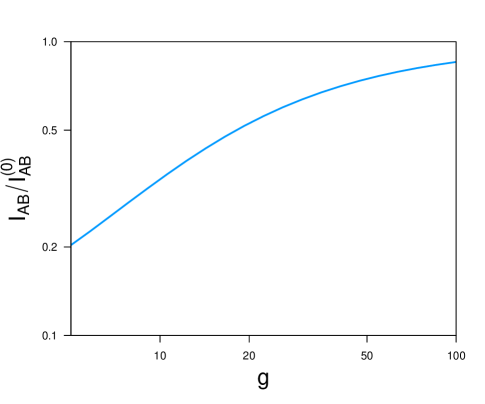
Figure 4: (Color online) The ratio $I_{AB}/I_{AB}^{(0)}$ as a function of dimensionless conductance $g$ at $T=0$ and $\tau_{D}/\tau_{RC}=10$.

The ratio $I_{AB}/I_{AB}^{(0)}$ was also evaluated numerically as a function of temperature at different values of $g$. The corresponding results are presented in Fig. 3. We observe that – in accordance with the above analytic expressions – the ratio $I_{AB}/I_{AB}^{(0)}$ grows with decreasing $T$ as a power law and finally saturates to a constant value smaller than unity at $T\lesssim 1/\tau_{D}$. The suppression of AB oscillations – both at higher temperatures and at $T\to 0$ clearly depends on the interaction strength which is controlled by the parameter $1/g$ in our model. Fig. 4 demonstrates the dependence of $I_{AB}/I_{AB}^{(0)}$ on $g$ in the limit of zero temperature and for $\tau_{D}/\tau_{RC}=10$. While at moderate values of $g\sim 10\div 20$ interaction-induced suppression of $I_{AB}$ remains pronounced down to $T=0$, at weaker interactions ($g\gtrsim 100$) this effect becomes less significant and is merely important at higher temperatures, cf. Fig. 3.

In order to complete our analysis let us briefly address additional quantum corrections to the current $I_{WL1,2}$ in Eq. (40). Although these terms do not depend on $\Phi$ and, hence, are irrelevant for AB oscillations, they allow to establish a direct and transparent relation between the Aharonov-Bohm effect studied here and the phenomenon of weak localization in systems of metallic quantum dots with electron-electron interactions GZ08 ; GZ07 . With the aid of Eq. (39) one easily finds

$$\frac{I_{WL1}}{I_{AB}}=\frac{g_{t1}}{2g_{t2}},\;\;\;\;\frac{I_{WL2}}{I_{AB}}=\frac{g_{t2}}{2g_{t1}}.$$ (48)

Combining this equation with the above results for $I_{AB}$ we immediately identify the terms $I_{WL1}$ and $I_{WL2}$ as weak localization corrections to the current GZ08 ; GZ07 originating from the two central barriers in our structure. In addition, in the absence of the magnetic field $\Phi=0$ the total quantum correction to the current $\delta I(0)$ (40) exactly coincides with the weak localization correction to the current for two connected in series metallic quantum dots GZ08 ; GZ07 provided the two central barriers in Fig. 1 are viewed as a composite tunnel barrier with total dimensionless conductance $g_{t1}+g_{t2}$.

V Concluding remarks

The established relation between our present results and those obtained in Refs. GZ08, ; GZ07, helps to clarify the main physical reason for the effect of interaction-induced suppression of AB oscillations in our structure. In full analogy with the weak localization correction GZ08 ; GZ07 both at non-zero temperatures and $T=0$ this suppression is due to electron dephasing by electron-electron interactions. This decoherence effect reduces the electron ability to interfere and, hence, decreases the amplitude $I_{AB}$ below its non-interacting value $I_{AB}^{(0)}$. At the same time Coulomb blockade effect – although yields an additional suppression of $I_{AB}$ – remains weak in metallic quantum dots and can be neglected as compared to the dominating effect of electron dephasing. It is also important to emphasize that in the course of our analysis we employed only one significant approximation: We performed a regular expansion of the current in powers of the tunneling conductances up to second order terms (forth order terms in the tunneling matrix elements). At the same time the effect of electron-electron interactions on AB oscillations in our system was treated non-perturbatively to all orders and essentially exactly.

Note that one could be tempted to interpret the suppression of $I_{AB}$ at $T=0$ just as a result of a simple renormalization effect by electron-electron interactions which is not related to dephasing. It is important to stress that – unlike, e.g., in the case of the interaction correction for single quantum dots GZ01 ; BN – here such interpretation would not be appropriate. The fundamental reason is that the interaction of an electron with an effective environment (produced by other electrons) effectively breaks down the time-reversal symmetry and, hence, causes both dissipation and dephasing for interacting electrons down to $T=0$ GZ98 . In this respect it is also important to point out a deep relation between interaction-induced electron decoherence and the $P(E)$-theory SZ ; IN which we already emphasized elsewhere GZ99 ; GZ08 ; GZ07 and which is also evident from our present results. Similarly to GZ08 ; GZ07 one can also introduce the electron dephasing time in our problem and demonstrate that at $T\to 0$ it saturates to a finite value in agreement with available experimental observations Pivin ; Huibers ; Hackens . We believe that the quantum dot rings considered here can be directly used for further experimental investigations of quantum coherence of interacting electrons in nanoscale conductors at low temperatures. We also note that our model can possibly be applied to analyze the behavior of recently fabricated self-assembled quantum rings Bel where the AB oscillations have been observed by means of magnetization experiments.

Acknowledgments

One of us (A.G.S.) acknowledges support from the Landau Foundation and from the Dynasty Foundation.

Appendix A Averaging over disorder

Let us consider the following disorder averages of the product for retarded and advanced Green functions for one of the quantum dots:

$$X_{d}({\bf x_{1}},{\bf x_{2}};\varepsilon)=\langle G^{R}({\bf x_{1}},{\bf x_{2}};\omega)G^{A}({\bf x_{2}},{\bf x_{1}};\omega-\varepsilon)\rangle_{d}-\langle G^{R}({\bf x_{1}},{\bf x_{2}};\omega)\rangle_{d}\langle G^{A}({\bf x_{2}},{\bf x_{1}};\omega-\varepsilon)\rangle_{d},$$ (49)

$$X_{c}({\bf x_{1}},{\bf x_{2}};\varepsilon)=\langle G^{R}({\bf x_{1}},{\bf x_{2}};\omega)G^{A}({\bf x_{1}},{\bf x_{2}};\omega-\varepsilon)\rangle_{d}-\langle G^{R}({\bf x_{1}},{\bf x_{2}};\omega)\rangle_{d}\langle G^{A}({\bf x_{1}},{\bf x_{2}};\omega-\varepsilon)\rangle_{d},$$ (50)

$$X_{k}({\bf x_{1}},{\bf x_{2}};\varepsilon)=\langle G^{R}({\bf x_{1}},{\bf x_{1}};\omega)G^{A}({\bf x_{2}},{\bf x_{2}};\omega-\varepsilon)\rangle_{d}-\langle G^{R}({\bf x_{1}},{\bf x_{1}};\omega)\rangle_{d}\langle G^{A}({\bf x_{2}},{\bf x_{2}};\omega-\varepsilon)\rangle_{d},$$ (51)

where

$$G^{R(A)}({\bf x_{1}}t_{1};{\bf x_{2}}t_{2})=\int\frac{d\omega}{2\pi}e^{-i\omega(t_{1}-t_{2})}G^{R(A)}({\bf x_{1}},{\bf x_{2}};\omega).$$ (52)

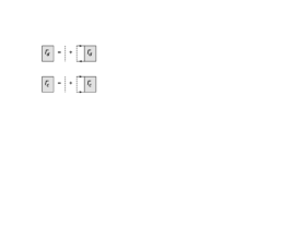
Figure 5: Diagrammatic representation for vertices $\Gamma_{d}({\bf x_{1}},{\bf x_{2}};\omega)$, $\Gamma_{c}({\bf x_{1}},{\bf x_{2}};\omega)$ and for averages $X_{d}({\bf x_{1}},{\bf x_{2}};\varepsilon)$ and $X_{c}({\bf x_{1}},{\bf x_{2}};\varepsilon)$.

In order to evaluate the above averages we will employ the standard diagram technique for noninteracting electrons in disordered systems AGD . The essential elements here are the so-called diffuson and Cooperon ladders depicted in Fig. 5 where we also define vertices $\Gamma_{d}({\bf x_{1}},{\bf x_{2}};\omega)$ and $\Gamma_{c}({\bf x_{1}},{\bf x_{2}};\omega)$. In the presence of time-reversal symmetry and in the limit of low momenta and frequencies these vertices obey a diffusion-like equation:

$$(-i\omega-D\nabla^{2}_{{\bf x_{2}}})\Gamma_{d(c)}({\bf x_{1}},{\bf x_{2}};\omega)=\frac{1}{2\pi N\tau_{e}^{2}}\delta({\bf x_{1}-x_{2}}).$$ (53)

Here $D=v_{F}l/3$ and $\tau_{e}=l/v_{F}$ are respectively the diffusion coefficient and the electron elastic mean free time. With the aid of the above vertices one can define the diffuson and the Cooperon respectively as

$$\mathcal{D}(t;{\bf x_{1}},{\bf x_{2}})=2\pi N\tau_{e}^{2}\int\frac{d\omega}{2\pi}e^{-i\omega t}\Gamma_{d}({\bf x_{1}},{\bf x_{2}};\omega),$$ (54)

$$\mathcal{C}(t;{\bf x_{1}},{\bf x_{2}})=2\pi N\tau_{e}^{2}\int\frac{d\omega}{2\pi}e^{-i\omega t}\Gamma_{c}({\bf x_{1}},{\bf x_{2}};\omega).$$ (55)

In the absence of the magnetic field they obey the following diffusion equations

$$(\partial_{t}-D\nabla^{2}_{{\bf x_{2}}})\mathcal{D}(t;{\bf x_{1}},{\bf x_{2}})=\delta({\bf x_{1}-x_{2}})\delta(t),$$ (56)

$$(\partial_{t}-D\nabla^{2}_{{\bf x_{2}}})\mathcal{C}(t;{\bf x_{1}},{\bf x_{2}})=\delta({\bf x_{1}-x_{2}})\delta(t)$$ (57)

with appropriate boundary conditions.

Evaluating the diagrams for $X_{d}({\bf x_{1}},{\bf x_{2}};\varepsilon)$ depicted in Fig. 5 after some algebra we arrive at the following result:

$$X_{d}({\bf x_{1}},{\bf x_{2}};\varepsilon)=(2\pi N\tau_{e})^{2}\Gamma_{d}({\bf x_{1}},{\bf x_{2}};\varepsilon)+(2\pi N\tau_{e})^{2}\varpi^{2}(|{\bf x_{1}}-{\bf x_{2}}|)\Gamma_{c}\left(\frac{{\bf x_{1}+x_{2}}}{2},\frac{{\bf x_{1}+x_{2}}}{2};\varepsilon\right),$$ (58)

where

$$\varpi(|{\bf x_{1}}-{\bf x_{2}}|)=\frac{1}{2\pi N\tau_{e}}\int d{\bf x}\langle G^{R}({\bf x_{1}},{\bf x};\omega)\rangle_{d}\langle G^{A}({\bf x},{\bf x_{2}};\omega)\rangle_{d}.$$ (59)

In the case of 3d systems we find $\varpi(r)=e^{-r/2l}\sin k_{F}r/k_{F}r$.

The expression for $X_{c}({\bf x_{1}},{\bf x_{2}};\varepsilon)$ is derived analogously. We find

$$X_{c}({\bf x_{1}},{\bf x_{2}};\varepsilon)=(2\pi N\tau_{e})^{2}\Gamma_{c}({\bf x_{1}},{\bf x_{2}};\varepsilon)+(2\pi N\tau_{e})^{2}\varpi^{2}(|{\bf x_{1}}-{\bf x_{2}}|)\Gamma_{d}\left(\frac{{\bf x_{1}+x_{2}}}{2},\frac{{\bf x_{1}+x_{2}}}{2};\varepsilon\right).$$ (60)

Combining Eqs. (49), (50, (52), (54), (55) with (58)-(60) we arrive at Eq. (25).

Figure 6: Diagrams which define the average $X_{k}({\bf x_{1}},{\bf x_{2}};\varepsilon)$.

Note that the average $X_{k}({\bf x_{1}},{\bf x_{2}};\varepsilon)$ (51) is omitted in Eq. (25) since this average turns out to be parametrically small as compared to both $X_{d}({\bf x_{1}},{\bf x_{2}};\varepsilon)$ and $X_{c}({\bf x_{1}},{\bf x_{2}};\varepsilon)$. In order to demonstrate this fact it is necessary to evaluate the diagrams for $X_{k}({\bf x_{1}},{\bf x_{2}};\varepsilon)$ depicted in Fig. 6. Proceeding as above we get

$$X_{k}({\bf x_{1}},{\bf x_{2}};\varepsilon)=(2\pi N\tau_{e})^{2}\varpi^{2}(|{\bf x_{1}}-{\bf x_{2}}|)\left[\Gamma_{d}\left(\frac{{\bf x_{1}+x_{2}}}{2},\frac{{\bf x_{1}+x_{2}}}{2};\varepsilon\right)+\Gamma_{c}\left(\frac{{\bf x_{1}+x_{2}}}{2},\frac{{\bf x_{1}+x_{2}}}{2};\varepsilon\right)\right]+$$

$$+(2\pi N\tau_{e}^{2})^{2}\left[\Gamma_{d}^{2}({\bf x_{1}},{\bf x_{2}};\varepsilon)+\Gamma_{c}^{2}({\bf x_{1}},{\bf x_{2}};\varepsilon)\right].$$ (61)

The first term in this equation clearly vanishes for $|{\bf x_{1}}-{\bf x_{2}}|\gtrsim l$. Here we assume that the size of both the dots and the contacts is large as compared to the electron mean free path $l$. Provided the typical contact size is of the same order as that of the dots the latter condition implies $l\ll v_{F}\tau_{D}$. If, however, the contact size is much smaller than that of the dots this condition becomes $p_{F}l\ll\sqrt{N_{ch}}$, where $N_{ch}$ is the effective number of conducting channels in the contact. In this case both the diffuson and the Cooperon do not depend on coordinates and are defined by Eq. (42). Then one finds

$$\Gamma_{d(c)}(\omega)=(2\pi N\tau_{e}\mathcal{V}(-i\omega+1/\tau_{D}))^{-1}.$$

Substituting this result into Eq. (61) we get $X_{k}(t)\approx\mathcal{V}^{-2}\theta(t)te^{-t/\tau_{D}}$. Comparing this expression with that for $X_{d}(c)(t)\approx 2\pi N\mathcal{V}^{-1}\theta(t)e^{-t/\tau_{D}}$ at times $t\lesssim\tau_{D}$ we obtain

$$X_{k}/X_{d(c)}\lesssim\tau_{D}/(N\mathcal{V})\sim\tau_{D}\delta\sim 1/g\ll 1.$$ (62)

This estimate demonstrates that the average $X_{k}$ (51) can be safely disregarded in Eq. (25) for the problem under consideration.

Appendix B Averaging over fluctuating phases

Substituting the action (26) into Eq. (29) one expresses the current $\delta I(\Phi)$ as a combination of different phase averages evaluated with the total action $S[\varphi^{+},\varphi^{-}]$. As we already argued above, in the metallic limit (1) all these averages are essentially Gaussian and, hence, can be easily performed. For the sake of completeness, below we present the corresponding results:

$$\langle e^{i(\varphi^{+}(t_{2})-\varphi^{+}(t_{3})+\varphi^{+}(t_{4})-\varphi^{+}(t_{1})+\frac{\varphi^{-}(t_{1})}{2}+\frac{\varphi^{-}(t_{2})}{2}+\frac{\varphi^{-}(t_{3})}{2}+\frac{\varphi^{-}(t_{4})}{2})}\rangle=$$

$$e^{-F(t_{1}-t_{2})-F(t_{1}-t_{4})-F(t_{2}-t_{3})-F(t_{3}-t_{4})+F(t_{1}-t_{3})+F(t_{2}-t_{4})}\times$$

$$\times e^{-iK(t_{1}-t_{2})-iK(|t_{1}-t_{3}|)-iK(t_{1}-t_{4})+iK(t_{2}-t_{3})+iK(|t_{2}-t_{4}|)-iK(t_{3}-t_{4})},$$ (63)

$$\langle e^{i(\varphi^{+}(t_{2})-\varphi^{+}(t_{3})+\varphi^{+}(t_{4})-\varphi^{+}(t_{1})+\frac{\varphi^{-}(t_{1})}{2}+\frac{\varphi^{-}(t_{2})}{2}+\frac{\varphi^{-}(t_{3})}{2}-\frac{\varphi^{-}(t_{4})}{2})}\rangle=$$

$$e^{-F(t_{1}-t_{2})-F(t_{1}-t_{4})-F(t_{2}-t_{3})-F(t_{3}-t_{4})+F(t_{1}-t_{3})+F(t_{2}-t_{4})}\times$$

$$\times e^{-iK(t_{1}-t_{2})-iK(|t_{1}-t_{3}|)-iK(|t_{1}-t_{4}|)+iK(t_{2}-t_{3})-iK(t_{2}-t_{4})+iK(|t_{3}-t_{4}|)},$$ (64)

$$\langle e^{i(\varphi^{+}(t_{2})-\varphi^{+}(t_{3})+\varphi^{+}(t_{4})-\varphi^{+}(t_{1})+\frac{\varphi^{-}(t_{1})}{2}+\frac{\varphi^{-}(t_{2})}{2}-\frac{\varphi^{-}(t_{3})}{2}+\frac{\varphi^{-}(t_{4})}{2})}\rangle=$$

$$e^{-F(t_{1}-t_{2})-F(t_{1}-t_{4})-F(t_{2}-t_{3})-F(t_{3}-t_{4})+F(t_{1}-t_{3})+F(t_{2}-t_{4})}\times$$

$$\times e^{-iK(t_{1}-t_{2})+iK(t_{1}-t_{3})-iK(t_{1}-t_{4})-iK(|t_{2}-t_{3}|)+iK(|t_{2}-t_{4}|)-iK(|t_{3}-t_{4}|)},$$ (65)

$$\langle e^{i(\varphi^{+}(t_{2})-\varphi^{+}(t_{3})+\varphi^{+}(t_{4})-\varphi^{+}(t_{1})+\frac{+\varphi^{-}(t_{1})}{2}-\frac{\varphi^{-}(t_{2})}{2}+\frac{\varphi^{-}(t_{3})}{2}-\frac{\varphi^{-}(t_{4})}{2})}\rangle=$$

$$e^{-F(t_{1}-t_{2})-F(t_{1}-t_{4})-F(t_{2}-t_{3})-F(t_{3}-t_{4})+F(t_{1}-t_{3})+F(t_{2}-t_{4})}\times$$

$$\times e^{-iK(t_{1}-t_{2})-iK(|t_{1}-t_{3}|)+iK(|t_{1}-t_{4}|)+iK(|t_{2}-t_{3}|)-iK(|t_{2}-t_{4}|)+iK(|t_{3}-t_{4}|)},$$ (66)

$$\langle e^{i(\varphi^{+}(t_{2})-\varphi^{+}(t_{3})+\varphi^{+}(t_{4})-\varphi^{+}(t_{1})+\frac{-\varphi^{-}(t_{1})}{2}+\frac{\varphi^{-}(t_{2})}{2}-\frac{\varphi^{-}(t_{3})}{2}+\frac{\varphi^{-}(t_{4})}{2})}\rangle=$$

$$e^{-F(t_{1}-t_{2})-F(t_{1}-t_{4})-F(t_{2}-t_{3})-F(t_{3}-t_{4})+F(t_{1}-t_{3})+F(t_{2}-t_{4})}\times$$

$$\times e^{-iK(|t_{1}-t_{2}|)+iK(|t_{1}-t_{3}|)-iK(|t_{1}-t_{4}|)-iK(|t_{2}-t_{3}|)+iK(|t_{2}-t_{4}|)-iK(|t_{3}-t_{4}|)},$$ (67)

$$\langle e^{i(\varphi^{+}(t_{2})-\varphi^{+}(t_{3})+\varphi^{+}(t_{4})-\varphi^{+}(t_{1})+\frac{\varphi^{-}(t_{1})}{2}+\frac{\varphi^{-}(t_{2})}{2}-\frac{\varphi^{-}(t_{3})}{2}-\frac{\varphi^{-}(t_{4})}{2})}\rangle=$$

$$e^{-F(t_{1}-t_{2})-F(t_{1}-t_{4})-F(t_{2}-t_{3})-F(t_{3}-t_{4})+F(t_{1}-t_{3})+F(t_{2}-t_{4})}\times$$

$$\times e^{-iK(t_{1}-t_{2})+iK(t_{1}-t_{3})+iK(|t_{1}-t_{4}|)+iK(|t_{2}-t_{3}|)-iK(|t_{2}-t_{4}|)+iK(|t_{3}-t_{4}|)}.$$ (68)

Note that for arbitrary metallic conductors $g_{L,R}\gg 1$ all these equations are accurate down to exponentially small energies (set by the so-called renormalized charging energy PZ91 ; Naz99 which is of little importance for us here), and in the particular limit of fully open left and right barriers Eqs. (63)-(68) become exact GGZ05 . Thus, combining (63)-(68) with Eqs. (26), (29), (37) and (38) we exactly account for the effect of electron-electron interactions on the amplitude of AB oscillations in the system under consideration.

It is useful to observe that in order to quantitatively describe this effect in the metallic limit $g\gg 1$ one can totally neglect all the functions $K(t)$ in all Eqs. (63)-(68). This is because these functions remain much smaller than one at all times (cf. Eq. (38)) and, hence, can only cause a weak ($\sim 1/g$) Coulomb correction to $I_{AB}$ which further slightly decreases the amplitude of AB oscillations. The origin of this Coulomb correction is exactly the same as that identified and discussed in the weak localization problem GZ08 ; GZ07 . Thus, no additional discussion of this point is necessary here.

Substituting unity instead of all the exponents in (63)-(68) containing $K$-functions and keeping all $F$-functions in the exponent, one easily arrives at Eq. (39).

References

(1) For a review see, e.g., A.G. Aronov and Yu.V. Sharvin,
Rev. Mod. Phys. 59, 755 (1987).
(2) For a review see, e.g., S. Chakravarty and A. Schmid,
Phys. Rep. 140, 193 (1986).
(3) D.S. Golubev and A.D. Zaikin, Phys. Rev. B 74, 245329 (2006).
(4) D.S. Golubev and A.D. Zaikin, New J. Phys. 10, 063027 (2008).
(5) D.S. Golubev and A.D. Zaikin, Physica E 40, 32 (2007).
(6) G. Schön and A.D. Zaikin, Phys. Rep. 198, 237 (1990).
(7) G.L. Ingold and Yu.V. Nazarov, Single Charge Tunneling,
(Plenum Press, New York) NATO ASI Series B 294, p. 21 (1992).
(8) D.S. Golubev and A.D. Zaikin, Quantum Physics at
Mesoscopic Scale (EDP Sciences, Les Ulis, 2000), p. 491.