Thermal effects in light scattering from ultracold bosons in an optical lattice

Abstract

We study the scattering of a weak and far-detuned light from a system of ultracold bosons in 1D and 3D optical lattices. We show the connection between angular distributions of the scattered light and statistical properties of a Bose gas in a periodic potential. The angular patterns are determined by the Fourier transform of the second-order correlation function, and thus they can be used to retrieve information on particle number fluctuations and correlations. We consider superfluid and Mott insulator phases of the Bose gas in a lattice, and we analyze in detail how the scattering depends on the system dimensionality, temperature and atom-atom interactions.

I Introduction

Experimental realization of Bose-Einstein condensates (BEC) in ultracold trapped gases opened up a rapidly expanding field of studies of quantum-degenerate systems Dalfovo et al. (1999); Giorgini et al. (2008); Bloch et al. (2008). Among the others, statistical properties of the condensate, such as its fluctuations and correlations, have attracted a wide attention. While the theory on this subject is well developed (see e.g. Idziaszek et al. (2009) and references therein), there are only few experiments that address this issue. To date, only the fluctuations of the total number of atoms in a condensed gas have been measured Chuu et al. (2005), and the subpoissonian scaling has been observed. The second order correlation functions, that are directly connected to the condensate atom number fluctuations, have been investigated experimentally in the collisions of metastable helium condensates et al. (2007) and in the expanding rubidium condensate Bucker et al. .

One of the potential tools to measure the statistics of quantum-degenerate gases is based on atom-light interactions.This possibility has been noticed already some time ago, and has been proposed for a detection of the Bose condensed phase Lewenstein and You (1993); Javanainen and Ruostekoski (1995); Saito and Ueda (1999); Moore and Meystre (1999), superfluidity in Fermi gases Zhang et al. (1999); Ruostekoski (1999); Törmä and Zoller (2000); Wong et al. (2000) and, quite recently, for a detection of quantum phases in ultracold gases in optical lattices Mekhov et al. (2007a, b); Chen et al. (2007); Eckert et al. (2007). The optical imaging techniques have already been used to measure coherence properties of BEC in the Raman superradiant scattering Sadler et al. (2007) and the second order correlation functions Bucker et al. .

The light scattered from a quantum gas carries information on atoms statistics, and thus can be used to measure the condensate fluctuations Idziaszek et al. (2000). In the case of BEC in a trap the profile of the scattered light is dominated by a component, which depends on the mean occupation number of the condensate. In order to detect a much weaker component resulting from fluctuations, one has to resort to the variance of the number of scattered photons, which can be difficult to measure.

The situation changes, however, in the presence of a periodic potential. In this case the dominating classical component exhibits interference pattern characteristic for the Bragg scattering, and the quantum component can be measured at the angles corresponding to destructive interference, where the large classical component vanishes. This property has been first noticed by Mekhov et al. Mekhov et al. (2007a), and these authors have proposed a method of probing the statistics of an ultracold gas in a lattice Mekhov et al. (2007c), based on the relatively strong coupling between atoms and light modes of a cavity. In this case one should be able to perform non-demolition measurement allowing to distinguish between superfluid and Mott-insulator (MI) quantum phases at temperature $T=0$.

In this paper we study a less complex situation of measuring a quantum gas statistics based on the far-off-resonance light scattering from a Bose gas in a lattice, focusing on the effects of statistics at finite temperatures. In order to avoid atom losses and suppress a possibility of perturbing the quantum state by the probing laser, we assume that the probing light is sufficiently weak and far-detuned. We show that the mean number of photons detected at some special angles, carries enough information not only to distinguish between different thermodynamic phases of the gas but also to directly measure the effects of the on-site atom statistics driven by quantum and thermal fluctuations. Hence, it allows to verify the validity of some well-grounded literature approaches, such as the Bogoliubov method, to describe higher order correlation functions in an interacting Bose gas.

Our paper is organized as follows. In section II we develop a model for scattering of light from ultracold atoms, showing that the number of scattered photons is directly related to the second-order correlation function. In section III we tailor our model to the external potential created by an optical lattice. The scattering from atoms in one dimensional (1D) lattice is considered in section IV, where for simplicity we focus only on the zero-temperature statistics discussing the effects of different approximations. The finite temperature statistics of a Bose gas in a lattice is analyzed in section V. Section VI investigates scattering from atoms in three-dimensional (3D) optical lattice at finite temperatures. We conclude in section VII, and finally two appendixes present technical details related to the influence of non-local Franck-Condon coefficients (Appendix A) and optimal configuration of a probing laser and a photon detector in the 3D lattice case (Appendix B).

II Interaction of light with many atoms

In this section we consider a general problem of light scattering from a gas of bosons in an arbitrary external potential. We assume that the trapped atoms are illuminated with a weak, and far-detuned laser light. The angularly resolved scattered light is measured by detectors in the far-field region. The full Hamiltonian of the system consists of the following parts:

$$\mathcal{H}=\mathcal{H}_{a}+\mathcal{H}_{f}+\mathcal{H}_{al}+\mathcal{H}_{af}$$ (1)

where $\mathcal{H}_{a}$ is the atomic Hamiltonian, $\mathcal{H}_{f}$ represents vacuum modes of the electromagnetic field (EM), $\mathcal{H}_{al}$ describes interaction of atoms with the laser light and $\mathcal{H}_{af}$ interaction of atoms with vacuum modes.

The atomic Hamiltonian can be split into two parts

$$\mathcal{H}_{a}=\mathcal{H}_{0}+\mathcal{H}_{int}$$ (2)

where $\mathcal{H}_{0}$ describes the system of two-level atoms in the second-quantization formalism Lewenstein et al. (1994)

$$\mathcal{H}_{0}=\sum\limits_{{\textbf{n}}}\hbar\omega^{g}_{{\textbf{n}}}g^{\dagger}_{{\textbf{n}}}g_{{\textbf{n}}}+\sum\limits_{{\textbf{m}}}\hbar\left(\omega_{{\textbf{m}}}^{e}+\omega_{0}\right)e^{\dagger}_{{\textbf{m}}}e_{{\textbf{m}}},$$ (3)

and the part including the atom-atom interactions reads

$$\mathcal{H}_{int}=\frac{1}{2}\sum\limits_{{\textbf{n}},{\textbf{m}},{\textbf{p}},{\textbf{q}}}U_{{\textbf{n}}{\textbf{m}}{\textbf{p}}{\textbf{q}}}\,g_{{\textbf{n}}}^{\dagger}g_{{\textbf{m}}}^{\dagger}g_{{\textbf{p}}}g_{{\textbf{q}}}.$$ (4)

Here, $g_{{\textbf{n}}}$ ($g^{\dagger}_{{\textbf{n}}}$) is the annihilation (creation) operator of an atom in the ground electronic state and state n of the center-of-mass (COM) motion, and $e_{{\textbf{m}}}$ ($e^{\dagger}_{{\textbf{m}}}$) is the annihilation (creation) operator of an atom in an electronic excited state and state m of COM motion. The operators obey the standard bosonic commutation relations: $[g_{{\textbf{n}}},g_{{\textbf{m}}}^{\dagger}]=\delta_{{\textbf{n}},{\textbf{m}}}$ and $[e_{{\textbf{n}}},e_{{\textbf{m}}}^{\dagger}]=\delta_{{\textbf{n}},{\textbf{m}}}$. The corresponding eigenenergies of atom COM motion are denoted by $\hbar\omega^{g}_{{\textbf{n}}}$ and $\hbar\omega_{{\textbf{m}}}^{e}$ for atoms in the ground and excited electronic states, respectively. The matrix elements $U_{{\textbf{n}}{\textbf{m}}{\textbf{p}}{\textbf{q}}}$ of the interaction Hamiltonian read

$$U_{{\textbf{n}}{\textbf{m}}{\textbf{p}}{\textbf{q}}}\equiv\frac{4\pi a_{s}\hbar^{2}}{m}\int d^{3}r\phi^{\ast}_{{\textbf{n}}}({\textbf{r}})\phi^{\ast}_{{\textbf{m}}}({\textbf{r}})\phi_{{\textbf{p}}}({\textbf{r}})\phi_{{\textbf{q}}}({\textbf{r}})$$ (5)

where we model short-range interactions through a contact potential with $s$-wave scattering length $a_{s}$ and a mass of the atom $m$. We neglect ground-excited and excited-excited atom interactions, assuming that for a weak and far-detuned probing light excited atoms constitute only a small fraction of the whole sample.

The Hamiltonian of the EM field takes a standard form:

$$\mathcal{H}_{f}=\sum\limits_{\lambda}\int d^{3}k\ \hbar\omega_{{\textbf{k}}}a^{\dagger}_{{\textbf{k}}\lambda}a_{{\textbf{k}}\lambda}$$ (6)

with $a_{{\textbf{k}}\lambda}$ ($a^{\dagger}_{{\textbf{k}}\lambda}$) being an annihilation (creation) operator of a photon with a wave vector k and a polarization $\lambda$.

The interaction of atoms with a laser beam is described as follows:

$$\mathcal{H}_{al}=\frac{\hbar\Omega}{2}\sum\limits_{{\textbf{n}},{\textbf{m}}}\langle{\textbf{n}},g|u_{{\textbf{k}}_{L}}({\textbf{r}})|{\textbf{m}},e\rangle e^{\imath\omega_{L}t}g^{\dagger}_{{\textbf{n}}}e_{{\textbf{m}}}+h.c.$$ (7)

where we treat the macroscopically occupied laser mode classically. Here, $u_{{\textbf{k}}_{L}}({\textbf{r}})$ characterizes a laser mode with a wave vector ${\textbf{k}}_{L}$, $\omega_{L}$ is the laser frequency, $\Omega$ is a Rabi frequency of the atomic transition, and the Franck-Condon coefficients $\langle{\textbf{n}},g|u_{{\textbf{k}}_{L}}({\textbf{r}})|{\textbf{m}},e\rangle$ describe a transition amplitude between COM motion states n and m of the atoms in the ground and excited electronic states, respectively. Typically, for a single probing laser, we have $u_{{\textbf{k}}_{L}}({\textbf{r}})=e^{\imath{\textbf{k}}_{L}{\textbf{r}}}$ (running wave), and for the two counter-propagating probing beams $u_{{\textbf{k}}_{L}}({\textbf{r}})=\cos\left({\textbf{k}}_{L}{\textbf{r}}\right)$ (standing wave). In general $u_{{\textbf{k}}_{L}}({\textbf{r}})$ can also represent the modes of an optical cavity Mekhov et al. (2007a).

The part of the Hamiltonian that describes coupling of atoms with quantized EM field is given by:

$$\mathcal{H}_{af} =\imath\sum\limits_{\lambda}\int d^{3}k\,\hbar c_{{\textbf{k}}\lambda}a^{\dagger}_{{\textbf{k}}\lambda}\sum\limits_{{\textbf{n}},{\textbf{m}}}\langle{\textbf{n}},g|u_{{\textbf{k}}}({\textbf{r}})|{\textbf{m}},e\rangle g^{\dagger}_{{\textbf{n}}}e_{{\textbf{m}}}$$

$$\phantom{=}+h.c.$$ (8)

in which $c_{{\textbf{k}}\lambda}=\sqrt{\omega_{{\textbf{k}}}/(16\pi^{3}\epsilon_{0}\hbar)}\left(\textbf{d}\cdot\mbox{\boldmath$\epsilon$}_{{\textbf{k}}\lambda}\right)$, d is a dipole moment of the atomic transition, $u_{{\textbf{k}}}({\textbf{r}})$ is a mode function of the EM field with a wavevector k and frequency $\omega_{{\textbf{k}}}$, and $\mbox{\boldmath$\epsilon$}_{\textbf{k}\lambda}$ is a unit vector perpendicular to k describing the mode of light with a polarization $\lambda$.

We solve the quantum equations of motion in the Heisenberg picture under the following approximation: i) we assume that the atomic operators are driven only by the dominating laser mode of the EM field, neglecting the back action of atoms on the laser mode, ii) the quantum dynamics of the vacuum modes is determined by the evolution of atomic operators, ignoring the back-action of the vacuum modes, which is equivalent to neglecting the process of spontaneous emission, iii) for the weak and far-detuned laser field we perform adiabatic elimination of the weakly populated excited state. Our approximations are analogous to those used in Idziaszek et al. (2000), with the only difference that here we perform the adiabatic elimination of the excited state, instead of assuming short probing pulses. We carry out our derivation neglecting the interactions between atoms and we comment on the generalization to the interacting gas case at the end of this section.

The equations of motion for the atomic operators in the interaction picture with respect to $\mathcal{H}_{0}$: $\tilde{g}_{\textbf{m}}(t)=g_{\textbf{m}}(t)e^{-\imath\omega_{\textbf{m}}^{g}t}$ and $\tilde{e}_{\textbf{n}}(t)=e_{\textbf{n}}(t)e^{-\imath(\omega_{\textbf{n}}^{e}+\omega_{0})t}$, read

$$\frac{d\tilde{g}_{\textbf{m}}}{d\tau} =-\imath\frac{\Omega}{2\Delta}\sum_{{\textbf{n}}}\eta_{{\textbf{n}}{\textbf{m}}}^{\ast}({\textbf{k}}_{L})\exp\left[\imath\frac{\omega_{\textbf{m}}^{g}-\omega_{\textbf{n}}^{e}+\Delta}{\Delta}\tau\right]\tilde{e}_{\textbf{n}}(\tau),$$ (9)

$$\frac{d\tilde{e}_{\textbf{n}}}{d\tau} =-\imath\frac{\Omega}{2\Delta}\sum_{{\textbf{m}}}\eta_{{\textbf{n}}{\textbf{m}}}({\textbf{k}}_{L})\exp\left[\imath\frac{\omega_{\textbf{n}}^{e}-\omega_{\textbf{m}}^{g}-\Delta}{\Delta}\tau\right]\tilde{g}_{\textbf{m}}(\tau),$$ (10)

where $\eta_{{\textbf{n}}{\textbf{m}}}({\textbf{k}})=\langle{\textbf{n}},e|u_{{\textbf{k}}}({\textbf{r}})|{\textbf{m}},g\rangle$, $\Delta=\omega_{L}-\omega_{0}$ and we have introduced rescaled time variable $\tau=\Delta t$. We solve Eqs. (9) and (10) by applying the Laplace transformation $F^{\cal L}(s)=\int_{0}^{\infty}d\tau\,e^{-s\tau}F(\tau)$. The Laplace transformed equations take the form

$$s\tilde{g}_{\textbf{m}}^{\cal L}(s)-\tilde{g}_{\textbf{m}}(0) =$$

$$-\imath\frac{\Omega}{2\Delta}\sum_{{\textbf{n}}} \eta_{{\textbf{n}}{\textbf{m}}}^{\ast}({\textbf{k}}_{L})\tilde{e}_{\textbf{n}}^{\cal L}(s)\left[s-\imath\frac{\omega_{\textbf{m}}^{g}-\omega_{\textbf{n}}^{e}+\Delta}{\Delta}\right],$$ (11)

$$s\tilde{e}_{\textbf{n}}^{\cal L}(s)-\tilde{e}_{\textbf{n}}(0) =$$

$$-\imath\frac{\Omega}{2\Delta}\sum_{{\textbf{m}}} \eta_{{\textbf{n}}{\textbf{m}}}({\textbf{k}}_{L})\tilde{g}_{\textbf{m}}^{\cal L}(s)\left[s-\imath\frac{\omega_{\textbf{n}}^{e}-\omega_{\textbf{m}}^{g}+\Delta}{\Delta}\right].$$ (12)

For a far-detuned light the prefactor on the right-hand-side of the equations is small: $\Omega/\Delta\ll 1$, and, in principle, the equations can be solved by iterations in a perturbative manner. Here, however, we proceed with solving Eq. (II) for $\tilde{e}_{\textbf{n}}^{\cal L}(s)$ and then substituting the result into Eq. (II). For a far-detuned light we apply $\Delta\gg\omega_{\textbf{n}}^{e},\omega_{\textbf{m}}^{g}$ and we use the identity $\displaystyle\sum_{{\textbf{n}}}\eta_{{\textbf{n}}{\textbf{m}}}^{\ast}({\textbf{k}}_{L})\eta_{{\textbf{n}}{\textbf{m}}^{\prime}}({\textbf{k}}_{L})=\delta_{{\textbf{m}}{\textbf{m}}^{\prime}}$, which results in

$$\tilde{g}^{\cal L}_{\textbf{m}}(s)\approx\frac{1}{s+\imath\frac{\Omega^{2}}{\Delta^{2}}}\left(\tilde{g}_{\textbf{m}}(0)-\imath\frac{\Omega}{2\Delta}\sum_{\textbf{n}}\eta_{{\textbf{n}}{\textbf{m}}}^{\ast}({\textbf{k}}_{L})\frac{\tilde{e}_{\textbf{n}}(0)}{s-\imath}\right).$$ (13)

By substituting back this result into Eq. (II), and performing the inverse Laplace transformation we obtain the following time-dependence of the atomic operators

$$\tilde{g}_{\textbf{m}}(t) =\tilde{g}_{\textbf{m}}(0)e^{-\imath\omega_{\mathrm{AC}}t}+{\cal O}\left(\frac{\Omega}{\Delta}\right),$$ (14)

$$\tilde{e}_{\textbf{n}}(t) =\tilde{e}_{\textbf{n}}(0)$$

$$\,+\frac{\Omega}{2\Delta}\sum_{\textbf{m}}\eta_{{\textbf{n}}{\textbf{m}}}({\textbf{k}}_{L})\tilde{g}_{\textbf{m}}(0)\left[e^{\imath(\omega_{\textbf{n}}^{e}-\omega_{\textbf{m}}^{g}-\Delta-\omega_{\mathrm{AC}})t}-1\right]$$

$$\,+{\cal O}\left(\frac{\Omega^{2}}{\Delta^{2}}\right),$$ (15)

Here, $\omega_{\mathrm{AC}}=\frac{\Omega^{2}}{4\Delta}$ denotes AC Stark shift of atomic levels in the field of the probing laser. In Eq. (14) we have not included terms of the order of $\Omega/\Delta$ , which are proportional to $\tilde{e}_{\textbf{n}}(0)$, since they do not give any contribution to the mean number of photons, assuming that there are no excited atoms at the beginning.

We substitute Eqs. (14) and (15) into equation of motion of the E-M field operators $\tilde{a}_{\textbf{k}\lambda}(t)=a_{\textbf{k}\lambda}(t)e^{-\imath\omega_{\textbf{k}}t}$ in the interaction picture. In the lowest order in $\Omega/\Delta$ this yields

$$\tilde{a}_{\textbf{k}\lambda}(t)-\tilde{a}_{\textbf{k}\lambda}(0)=\\ =c_{{\textbf{k}}\lambda}\frac{\Omega}{\Delta}\sum_{{\textbf{n}}{\textbf{n}}^{\prime}{\textbf{m}}}\eta_{{\textbf{m}}{\textbf{n}}^{\prime}}({\textbf{k}})\eta_{{\textbf{m}}{\textbf{n}}}^{\ast}({\textbf{k}}_{L})\tilde{g}^{\dagger}_{\textbf{n}}(0)\tilde{g}_{{\textbf{n}}^{\prime}}(0)\\ \times\frac{e^{\imath(\omega_{\textbf{k}}-\omega^{L}_{{\textbf{n}}{\textbf{n}}^{\prime}})t/2}}{\omega_{\textbf{k}}-\omega^{L}_{{\textbf{n}}{\textbf{n}}^{\prime}}}\sin\left(\frac{\omega_{\textbf{k}}-\omega^{L}_{{\textbf{n}}{\textbf{n}}^{\prime}}}{2}t\right)$$ (16)

where $\omega^{L}_{{\textbf{n}}{\textbf{n}}^{\prime}}\equiv\omega_{L}+\omega_{{\textbf{n}}^{\prime}}^{g}-\omega_{\textbf{n}}^{g}$. At $t\rightarrow\infty$ the sine term will produce a term proportional to the delta function, describing the energy conservation in the process of a single photon scattering: $\omega_{\textbf{k}}=\omega_{{\textbf{k}}_{L}}+\omega_{{\textbf{n}}^{\prime}}^{g}-\omega_{\textbf{n}}^{g}$. However, in our case we are interested in the total number of photons scattered into a given solid angle, and not in the spectrum of the scattered light. Hence, we use the approximation $\omega^{L}_{{\textbf{n}}{\textbf{n}}^{\prime}}\approx\omega_{L}$. This condition is also applicable in the physical systems where the natural linewidth $\Gamma$ associated with the atomic transition is broader than frequencies of atom COM motion: $\Gamma\gg\omega_{\textbf{n}}^{g}$.

Now, by using Eq. (16) and approximation $\omega^{L}_{{\textbf{n}}{\textbf{n}}^{\prime}}\approx\omega_{L}$ we calculate the mean number of photons with a wavevector k and a polarization $\lambda$

$$\!\!\left\langle a^{\dagger}_{{\textbf{k}}\lambda}\left(t\right)a_{{\textbf{k}}\lambda}\left(t\right)\right\rangle=\frac{\Omega^{2}c_{{\textbf{k}}\lambda}^{2}}{\Delta^{2}}\frac{\sin^{2}\left(\left(\omega_{{\textbf{k}}}-\omega_{L}\right)t/2\right)}{\left(\omega_{{\textbf{k}}}-\omega_{L}\right)^{2}}F({\textbf{k}},{\textbf{k}}_{L}),$$ (17)

where the function $F({\textbf{k}},{\textbf{k}}_{L})$ is defined as follows:

$$F({\textbf{k}},{\textbf{k}}_{L})\equiv \sum_{\begin{subarray}{c}{{\textbf{n}}},{{\textbf{n}}}^{\prime}\\ {{\textbf{m}}},{{\textbf{m}}}^{\prime}\end{subarray}}\langle{\textbf{n}}|u_{{\textbf{k}}}^{\ast}({{\textbf{r}}})u_{{\textbf{k}}_{L}}({{\textbf{r}}})|{\textbf{n}}^{\prime}\rangle\langle{\textbf{m}}|u_{{\textbf{k}}}({\textbf{r}})u_{{\textbf{k}}_{L}}^{\ast}({\textbf{r}})|{\textbf{m}}^{\prime}\rangle$$

$$\times\left\langle g_{{\textbf{n}}}^{\dagger}(0)g_{{\textbf{n}}^{\prime}}(0)g_{{\textbf{m}}}^{\dagger}(0)g_{{\textbf{m}}^{\prime}}(0)\right\rangle.$$ (18)

Notice that, in Eq. (18) all the matrix elements are calculated between COM states of ground-state atoms $|{\textbf{n}},g\rangle$ and to shorten the notation $|{\textbf{n}}\rangle\equiv|{\textbf{n}},g\rangle$. In the particular case when the mode functions $u_{{\textbf{k}}}({\textbf{r}})$ and $u_{{\textbf{k}}_{L}}({\textbf{r}})$ are the plane waves, $F({\textbf{k}},{\textbf{k}}_{L})$ reduces to the Fourier transform of the second-order correlation function in atomic field operators $\hat{\Psi}_{g}({\textbf{x}})$ of the atoms in the electronic ground state

$$F({\textbf{q}})=\int\!\!d^{3}x\int\!\!d^{3}y\,e^{\imath{\textbf{q}}({\textbf{x}}-{\textbf{y}})}\left\langle\hat{\Psi}_{g}^{\dagger}({\textbf{x}})\hat{\Psi}_{g}({\textbf{x}})\hat{\Psi}_{g}^{\dagger}({\textbf{y}})\hat{\Psi}_{g}({\textbf{y}})\right\rangle$$ (19)

where ${\textbf{q}}={\textbf{k}}-{\textbf{k}}_{L}$ is the wave vector of the momentum transfer. In the rest of the paper we will use the $F({\textbf{q}})$ function only.

An analogous result is obtained when considering the scattering of neutrons from liquid helium Van Hove (1954). In that case the number of scattered particles associated with the momentum transfer q and the energy transfer to the system $\hbar\omega$ is described by the dynamic structure factor

$$S({\textbf{q}},\omega)\equiv\frac{1}{N}\int\!\!d^{3}x\!\!\int\!\!d^{3}y\,\,e^{\imath{\textbf{q}}({\textbf{x}}-{\textbf{y}})}\\ \times\langle\Psi_{E}|\hat{\rho}({\textbf{x}})\delta(H-E-\hbar\omega)\hat{\rho}({\textbf{x}})|\Psi_{E}\rangle$$ (20)

where $\hat{\rho}({\textbf{x}})=\hat{\Psi}^{\dagger}({\textbf{x}})\hat{\Psi}({\textbf{x}})$, $H$ is the Hamiltonian of the system, and $|\Psi_{E}\rangle$ is an eigenstate with energy $E$. By integrating over energies of the scattered particles one obtains the static structure factor

$$S({\textbf{q}})=\hbar\int_{-\infty}^{\infty}d\omega\,S({\textbf{q}},\omega)$$ (21)

which is equivalent to our function $F({\textbf{q}})$ describing an amplitude of scattered photons integrated over photon frequencies rem (a). We will refer to $F({\textbf{q}})$ as the structure function in the rest of the paper.

For evolution time $t$ much longer than the time scale determined by the optical frequencies $\omega_{L}$, we can apply the following identity

$$\lim_{t\rightarrow\infty}\frac{\sin^{2}\left(\left(\omega_{{\textbf{k}}}-\omega_{L}\right)t/2\right)}{t\left(\omega_{{\textbf{k}}}-\omega_{L}\right)^{2}}=\frac{\pi}{2}\,\delta\left(\omega_{{\textbf{k}}}-\omega_{L}\right),$$ (22)

to show that for the weak and far-detuned laser the scattered light described by Eq. (17) has spectrum centered around elastic component.

The total number of photons scattered into a solid angle $d\Omega$ is equal to

$$\frac{dN_{ph}}{d\Omega}(\hat{{\textbf{k}}})=\sum\limits_{\lambda}\int\!\!dk\;k^{2}\left\langle a^{\dagger}_{{\textbf{k}}\lambda}\left(t\right)a_{{\textbf{k}}\lambda}\left(t\right)\right\rangle$$ (23)

where $\hat{{\textbf{k}}}={\textbf{k}}/|{\textbf{k}}|$ represents the direction of measurement. Since, according to Eq. (22), the number of photons is proportional to pulse length as expected, it is more convenient to calculate the number of photons scattered into $d\Omega$ per unit of time

$$\frac{d^{2}N_{ph}}{d\Omega dt}({\textbf{k}},{\textbf{k}}_{L}) =\frac{\Omega^{2}\omega_{L}^{3}d^{2}}{32\pi^{2}\Delta^{2}\epsilon_{0}\hbar c^{3}}{\cal W}(\hat{{\textbf{k}}})F({\textbf{k}}-{\textbf{k}}_{L})$$

$$=\left[\frac{d^{2}N_{ph}}{d\Omega dt}({\textbf{k}},{\textbf{k}}_{L})\right]_{\begin{subarray}{c}\!\!\mathrm{one}\\ \mathrm{atom}\end{subarray}}F({\textbf{q}})$$ (24)

where ${\cal W}(\hat{{\textbf{k}}})=\left(1-(\mbox{\boldmath$\epsilon$}_{\textbf{d}}\cdot\mbox{\boldmath$\epsilon$}_{\textbf{k}})^{2}\right)$ is the dipole pattern of the emitted light and ${\textbf{\mbox{\boldmath$\epsilon$}}}_{\textbf{d}}$ is a unit vector in the direction of the dipole moment d that is determined by a polarization of the probing laser. Eq. (24) shows that the angular distribution of the scattered light, apart from the contribution from the dipole pattern, is determined only by $F({\textbf{q}})$. In addition, for a single atom $F({\textbf{q}})~{}=~{}1$ and thus all the information about scattering from the system of $N$ atoms is contained in $F({\textbf{q}})$. Therefore, in the subsequent sections, we can focus solely on the properties of $F({\textbf{q}})$, keeping in mind that the remaining contribution is the same as for the scattering from a single atom.

The generalization of our derivation to the case of interacting atoms can be performed in an analogy to the problem of neutron scattering from liquid helium Van Hove (1954); Pitaevskii and Stringari (2003). If one applies the Born approximation, and eliminates adiabatically the excited state, one ends up with the result identical to the one presented here. A similar approach has been applied to the study of Raman scattering in the superradiant regime Uys and Meystre (2008).

Finally we note that our perturbative treatment neglects the effects of the momentum transfer resulting from the photon recoil in the process of light scattering. We assume, however, that the scattered light is weak and far-detuned, therefore we expect that the fraction of atoms which experience the photon recoil is sufficiently small, such that the atom statistics is not significantly affected. Moreover, in the presence of a tight trapping potential, such as a deep optical lattice, one finds that the scattering is recoilless Gajda et al. (1996), which requires the trap size smaller than a wave length of the scattered light.

III Scattering from ultracold gas of bosons in an optical lattice

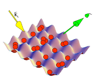
Figure 1: (Color online) Setup. An ultracold gas of bosons confined in an optical lattice is illuminated with a probing laser beam (yellow arrow) characterized by the wavevector ${\textbf{k}}_{L}$. The photons scattered into a selected direction (green arrow) are collected by a detector.

The setup we consider is schematically plotted in Fig. 1. It consists of an ultracold gas of $N$ bosons confined in an optical cubic lattice of $M$ sites. We assume a homogeneous system with an equal average number of atoms $n=N/M$ in each site of a lattice. The periodic potential of the lattice reads Bloch et al. (2008):

$$V_{p}(x,y,z)=V_{0}\left(\sin^{2}k_{p}x+\sin^{2}k_{p}y+\sin^{2}k_{p}z\right)$$ (25)

where ${\textbf{k}}_{p}$ is a wave vector of laser beams that are used to form the lattice and $V_{0}$ is the potential depth. The exact configuration of the probing beam and detectors will depend on a dimensionality of the lattice and will be discussed later. In order to use the results of the previous section, we need to specify a single-particle basis. In the case of atoms confined in an optical lattice it is convenient to choose the basis of Wannier functions $w_{\textbf{m}}({\textbf{r}})$ that represent wave functions localized at single lattice sites m and are linear combinations of Bloch states. In our approach we consider only excitations within the lowest Bloch band, so in a limit of deep optical lattices the Wannier functions describe only the ground state wave functions in local potential wells.

III.1 Deep lattice regime

For a deep optical lattice, the Wannier states are well localized within the sites of the lattice, and in equation (18) we can restrict to optical transitions between the states localized at the same lattice sites: ${\textbf{n}}={\textbf{n}}^{\prime}$ and ${\textbf{m}}={\textbf{m}}^{\prime}$. In this case $F({\textbf{q}})$ simplifies to the following expression

$$F({\textbf{q}}) =\sum\limits_{{\textbf{n}},{\textbf{m}}}\langle{\textbf{n}}|e^{\imath{\textbf{q}}{\textbf{r}}}|{\textbf{n}}\rangle\langle{\textbf{m}}|e^{-\imath{\textbf{q}}{\textbf{r}}}|{\textbf{m}}\rangle\left\langle g_{{\textbf{n}}}^{\dagger}g_{{\textbf{n}}}g_{{\textbf{m}}}^{\dagger}g_{{\textbf{m}}}\right\rangle$$

$$=\left|f_{\textbf{0},\textbf{0}}({\textbf{q}})\right|^{2}\sum\limits_{{\textbf{n}},{\textbf{m}}}e^{\imath{\textbf{q}}\left({\textbf{r}}_{{\textbf{n}}}-{\textbf{r}}_{{\textbf{m}}}\right)}\left\langle n_{{\textbf{n}}}n_{{\textbf{m}}}\right\rangle$$ (26)

where $n_{{\textbf{m}}}\equiv g_{{\textbf{m}}}^{\dagger}g_{{\textbf{m}}}$ and

$$f_{{\textbf{n}},{\textbf{m}}}({\textbf{q}})\equiv\langle{\textbf{n}}|e^{\imath{\textbf{q}}{\textbf{r}}}|{\textbf{m}}\rangle=\int d^{3}r\,w^{\ast}_{{\textbf{n}}}({\textbf{r}})e^{\imath{\textbf{q}}{\textbf{r}}}w_{{\textbf{m}}}({\textbf{r}}).$$ (27)

In analogy to the scattering of light into an optical cavity Mekhov et al. (2007c), we can define the classical part $F^{clas}({\textbf{q}})$ and the quantum part $F^{quant}({\textbf{q}})$ of the function $F({\textbf{q}})$

$$F^{clas}({\textbf{q}}) \equiv n^{2}\left|f_{\textbf{0},\textbf{0}}({\textbf{q}})\right|^{2}\left|\sum\limits_{{\textbf{m}}}e^{\imath{\textbf{q}}{\textbf{r}}_{{\textbf{m}}}}\right|^{2},$$ (28)

$$F^{quant}({\textbf{q}}) \equiv F({\textbf{q}})-F^{clas}({\textbf{q}})$$

$$=\left|f_{\textbf{0},\textbf{0}}({\textbf{q}})\right|^{2}\sum\limits_{{\textbf{n}},{\textbf{m}}}e^{\imath{\textbf{q}}\left({\textbf{r}}_{{\textbf{n}}}-{\textbf{r}}_{{\textbf{m}}}\right)}\left(\left\langle n_{{\textbf{n}}}n_{{\textbf{m}}}\right\rangle-n^{2}\right).$$ (29)

The former yields the classical amplitude of the scattered light $\left|\left\langle a_{{\textbf{k}}\lambda}\right\rangle\right|^{2}$, whereas the latter represents the remaining quantum contribution that together with $F^{clas}({\textbf{q}})$ sum up to the total number of photons $\left\langle a_{{\textbf{k}}\lambda}^{\dagger}a_{{\textbf{k}}\lambda}\right\rangle$. We note that $F^{clas}({\textbf{q}})$ has a form characteristic for a Bragg scattering and it is not affected by any statistical properties of the ultracold gas of bosons. On the contrary, $F^{quant}({\textbf{q}})$ is sensitive to the atom number statistics and thus enables us to investigate statistical properties of different quantum states.

IV Scattering from a Bose gas in one-dimensional optical lattice at zero temperature

The geometry of the system we investigate in this section is depicted in Fig. 2. We consider one-dimensional homogeneous optical lattice generated by two overlapping and counterpropagating laser beams characterized by the wavelength $\lambda_{p}$. Atoms confined to the periodic potential are illuminated with a single laser beam with the wavelength $\lambda_{L}$. For the single particle basis that we have chosen the states

$$\psi_{m}({\textbf{r}})=w_{m}(z)\,\psi_{\scriptscriptstyle{\perp}}(x,y)$$ (30)

are products of a Wannier function $w_{m}(z)$ localized at lattice site $m$ along $z$-direction, and a Gaussian function $\psi_{\scriptscriptstyle{\perp}}(x,y)$ in tightly confined, perpendicular direction. For simplicity we assume the cylindrical symmetry $\psi_{\scriptscriptstyle{\perp}}(x,y)=\psi_{\scriptscriptstyle{\perp}}(\rho)$.

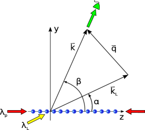
Figure 2: (Color online) Setup. A quasi one-dimensional optical lattice is illuminated with a probing laser set at an angle $\alpha\,\epsilon\,[-\pi,\pi[$. A detector is set at an angle $\beta\,\epsilon\,[-\pi,\pi[$.

At zero temparature a gas of bosons in a periodic potential appears in two distinct quantum phases Fisher et al. (1989); Jaksch et al. (1998). When the tunneling process dominates over the on-site atom repulsion the system is found in the superfluid (SF) phase that is characterized by the presence of a global coherence and a non-zero order parameter. In contrast, for the on-site interactions stronger than the tunneling rate, the system exhibits the Mott-insulator phase. In the latter case the global coherence is lost, while the on-site particle number is fixed and the on-site fluctuations are suppressed.

For a Bose gas at zero temperature and deep in the MI regime, the on-site fluctuations and correlations vanish: $\left\langle n_{m}n_{m^{\prime}}\right\rangle-\left\langle n_{m}\right\rangle\left\langle n_{m^{\prime}}\right\rangle=0$. Hence, the quantum part $F^{quant}({\textbf{q}})$ is zero identically, and the scattering is described by the standard Bragg pattern with characteristic set of maxima and minima, corresponding to the directions of constructive and destructive interference. In contrast, SF phase at $T=0$ exhibits nonzero fluctuations and correlations: $\left\langle n_{m}n_{m^{\prime}}\right\rangle-\left\langle n_{m}\right\rangle\left\langle n_{m^{\prime}}\right\rangle=n\delta_{mm^{\prime}}-\frac{n^{2}}{N}$. Hence, apart from the similar behavior of the classical part $F^{clas}({\textbf{q}})$ as for MI phase, the SF phase also gives rise to nonzero quantum component $F^{quant}({\textbf{q}})$ which, within the deep lattice approximation (Eq. (26)), is given by $F^{quant}({\textbf{q}})=N\left|f_{0,0}({\textbf{q}})\right|^{2}$. This offers a unique possibility of a non-destructive measurement that allows one to distinguish between SF and MI phases Mekhov et al. (2007a).

Fig. 4 and Fig. 4 compare the scattering patterns from the SF and MI phases for the systems of $M=55$ sites with different configurations of the probing laser and different ratios of $\lambda_{p}$ to $\lambda_{L}$. At some characteristic angles corresponding to the Bragg scattering minima due to the destructive interference, the scattering from the MI state vanishes. In contrast, the scattering pattern from the SF state is nonzero at all angles, also in the directions where the classical component vanishes. We observe that a change of a ratio $\lambda_{p}/\lambda_{L}$ affects the scattering pattern, in particular a number and positions of the highest peaks resulting from the constructive interference.

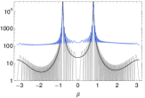
(a)  $\alpha=\pi/4$

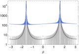
(b)  $\alpha=\pi/2$

Figure 3: (Color online) Structure function $F({\textbf{q}})$ for SF (blue top curve) and MI (gray bottom curve) phases, in the deep lattice approximation, for a probing laser set at different angles $\alpha$, and a detector set at angle $\beta$. Here, $V_{0}=15E_{r}$, $M=55$, $N=3M$, $\lambda_{p}/\lambda_{L}=1$. The black line represents average distribution (32).

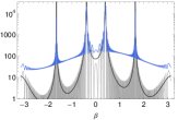
(a)  $\lambda_{p}/\lambda_{L}=2$

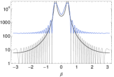
(b)  $\lambda_{p}/\lambda_{L}=1/3$

Figure 4: (Color online) Structure function $F({\textbf{q}})$ for SF (blue top curve) and MI (gray bottom curve) phases, in the deep lattice approximation, for different ratios of $\lambda_{p}/\lambda_{L}$, and a detector set at angle $\beta$. Here, $V_{0}=10E_{r}$, $M=55$, $N=3M$, $\alpha=\pi/8$. The black line represents the average distribution (32).

We note that for large $M$ the scattering pattern quickly oscillates and thus, in the realistic measurement, one would detect photons scattered in some finite solid angle $d\Omega$ which is characteristic for the detector and that contains several interference fringes. Hence, we find it more appropriate to calculate the angular distribution of photons that is averaged over few neighboring maxima. The averaging does not affect the scattering pattern of SF phase, which is rather smooth, but it is important for MI phase. In 1D optical lattice, the angular distribution of photons scattered from MI state is determined by

$$F^{MI}({\textbf{q}})=\left|f_{0,0}({\textbf{q}})\right|^{2}n^{2}\frac{\sin^{2}\left(\frac{M}{2}{\textbf{q}}{\textbf{d}}\right)}{\sin^{2}\left(\frac{1}{2}{\textbf{q}}{\textbf{d}}\right)}$$ (31)

where d denotes the translation vector of a 1D lattice. Averaging over some finite solid angle around q containing several maxima yields

$$\overline{F^{MI}({\textbf{q}})}=\left|f_{0,0}({\textbf{q}})\right|^{2}\frac{n^{2}}{2}\frac{1}{\sin^{2}\left(\frac{1}{2}{\textbf{q}}{\textbf{d}}\right)}.$$ (32)

The above result is derived provided that the measurement is done not too close to the main maxima determined by the directions of the constructive interference. As can be observed in Fig. 4 and Fig. 4, the averaged distribution of the light scattered from MI phase still can be well distinguished from the scattering from the SF phase, and result (32) for the averaged distribution remains approximately valid even close to the points of the destructive interference.

While performing the deep lattice approximation in Eq. (26) we have dropped all the Franck-Condon factors corresponding to transitions between states localized in different lattice sites. Obviously, with the decreasing lattice depth, the Wannier states begin to overlap between neighboring sites and we expect the nonlocal Franck-Condon factors to give larger contribution. In order to investigate this issue in Fig. 5 we compare the deep lattice approximation (26) with the result that includes summation over all pairs of the lattice sites in Eq. (18). For the clarity of presentation we show the results for a relatively small system of $M=11$ sites and a lattice depth $V=1E_{r}$ and $V=5E_{r}$ for SF and MI phases, respectively, expressed in the units of the recoil energy $E_{r}=\hbar^{2}k_{L}^{2}/(2m)$. We observe that even for the shallow lattice potential the nonlocal corrections give negligible contribution for the scattering from the SF state. Moreover, for the MI state the nonlocal corrections are even smaller because of the deeper lattice required to achieve this phase. In Appendix A we show that corrections due to the nearest neighbors in weak lattices are isotropic and scale as the total number of atoms $N$. Therefore, nonlocal corrections give rise to a scattering at the angles of destructive interference of the classical part. However, for typical lattice depths, the corresponding contribution is small and can be totally neglected for both quantum phases.

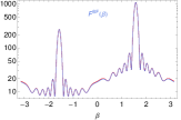
(a)   SF scattering at $V_{0}=1E_{r}$

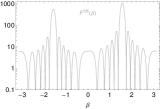
(b)   MI scattering at $V_{0}=5E_{r}$

Figure 5: (Color online) Distribution of light scattered from SF (left panel) and MI (right panel) phases at zero temperature, versus the angle $\beta$. Here, $M=11$, $N=3M$, $\alpha=\pi/2$, and $\lambda_{p}/\lambda_{L}=1$. The red curves present $F(\beta)$ calculated in local approximation (26), whereas the blue curve (in the SF case) and the gray curve (in the MI case) show results including also non-local Franck-Condon factors as in Eq. (18). In the case of scattering from the SF state at $V_{0}=1E_{r}$ one notices slight differences between the two curves in a vicinity of $\beta=0$ and $\beta=\pm\pi$. In the case of scattering from the MI state at $V_{0}=5E_{r}$ the two curves are indistinguishable.

V Statistical properties at finite temperatures

V.1 Bose-Hubbard model of an ultracold gas in a periodic potential

As discussed in the previous section, the angular distribution of the scattered light is determined by the occupation number statistics in lattice sites. We investigate the occupation number statistics within Bose-Hubbard (BH) model Fisher et al. (1989); Jaksch et al. (1998), considering only excitations within the lowest Bloch band. The BH Hamiltonian reads:

$$\mathcal{H}=-J\!\!\!\!\sum\limits_{\left\langle{\textbf{m}},{\textbf{m}}^{\prime}\right\rangle}g^{\dagger}_{{\textbf{m}}}g_{{\textbf{m}}^{\prime}}+\frac{1}{2}U\!\sum\limits_{{\textbf{m}}}\hat{n}_{{\textbf{m}}}\left(\hat{n}_{{\textbf{m}}}-1\right)$$ (33)

where the first sum on the right-hand side is restricted to nearest neighbors only. The parameter

$$J\equiv-\int d^{3}r\>w^{\ast}_{{\textbf{m}}}({\textbf{r}})\left[-\frac{\hbar^{2}}{2m}\nabla^{2}+V_{p}({\textbf{r}})\right]w_{{\textbf{m}}^{\prime}}({\textbf{r}})$$ (34)

is the hopping matrix element between neighboring sites m and ${\textbf{m}}^{\prime}$, and parameter:

$$U\equiv\frac{4\pi a_{s}\hbar^{2}}{m}\int d^{3}r\left|w_{{\textbf{m}}}({\textbf{r}})\right|^{4}$$ (35)

corresponds to the strength of the on site repulsion of two atoms in a lattice site m. As before, $w_{{\textbf{m}}}({\textbf{r}})$ is the single-particle Wannier’s wavefunction of an atom occupying site m in a lattice.

The BH Hamiltonian can be equivalently expressed in the momentum space, which is convenient for the analysis of the SF phase at finite temperatures and application of the Bogoliubov method. To this end we introduce annihilation and creation operators in momentum space

$$a_{{\textbf{k}}}= \frac{1}{\sqrt{M}}\sum\limits_{{\textbf{m}}}g_{{\textbf{m}}}e^{\imath{\textbf{k}}{\textbf{r}}_{{\textbf{m}}}},$$ (36)

$$a^{\dagger}_{{\textbf{k}}}= \frac{1}{\sqrt{M}}\sum\limits_{{\textbf{m}}}g^{\dagger}_{{\textbf{m}}}e^{-\imath{\textbf{k}}{\textbf{r}}_{{\textbf{m}}}},$$ (37)

respectively, in which index m runs over all sites in a lattice. A period of the cubic lattice is $d=\lambda_{p}/2$ and a size of the system is equal to $L=M^{1/3}d$. The periodic boundary conditions imply quantization of a wave vector: $\;{\textbf{k}}=\frac{2\pi}{L}(n_{x},n_{y},n_{z})$, where $n_{i}$ are integer numbers ranging from $-\lfloor M/2\rfloor$ to $\lfloor M/2\rfloor$ rem (b). By rewriting Eq. (33) in terms of $a_{{\textbf{k}}}$ and $a^{\dagger}_{{\textbf{k}}}$, we find:

$$\mathcal{H}= \sum\limits_{{\textbf{k}}}\epsilon_{{\textbf{k}}}a^{\dagger}_{{\textbf{k}}}a_{{\textbf{k}}}+\frac{U}{2M}\sum\limits_{{\textbf{k}},{\textbf{k}}^{\prime},{\textbf{k}}^{\prime\prime}}a^{\dagger}_{{\textbf{k}}+{\textbf{k}}^{\prime\prime}}a^{\dagger}_{{\textbf{k}}^{\prime}-{\textbf{k}}^{\prime\prime}}a_{{\textbf{k}}^{\prime}}a_{{\textbf{k}}}$$ (38)

where

$$\epsilon_{{\textbf{k}}}\equiv 6J-2J\sum\limits_{i=1}^{3}\cos\left(k_{i}d\right).$$ (39)

V.2 Statistical properties of the superfluid phase

The standard description of a weakly interacting Bose gas is based on the Bogoliubov approximation Bogoliubov (1947) and can be also applied for a superfluid phase in periodic potentials van Oosten et al. (2001). We perform the Bogoliubov approximation to Hamiltonian (38), replacing the annihilation and creation operators in the zero quasi-momentum modes (${\textbf{k}}=0$) by $\mathbb{C}$-numbers $a_{0}\approx a_{0}^{\dagger}\approx\sqrt{N_{0}}$. By introducing the quasi-particle annihilation and creation operators $b_{{\textbf{k}}}$ and $b^{\dagger}_{{\textbf{k}}}$, respectively, which fulfill the standard bosonic commutation rules $\left[b_{{\textbf{k}}},b^{\dagger}_{{\textbf{k}}^{\prime}}\right]=\delta_{{\textbf{k}},{\textbf{k}}^{\prime}}$, and are related to $a_{{\textbf{k}}}$ and $a^{\dagger}_{{\textbf{k}}}$ by the canonical transformation

$$\begin{pmatrix}b_{{\textbf{k}}}\\ b^{\dagger}_{-{\textbf{k}}}\end{pmatrix}=\begin{pmatrix}u_{{\textbf{k}}}&v_{{\textbf{k}}}\\ v_{{\textbf{k}}}&u_{{\textbf{k}}}\end{pmatrix}\begin{pmatrix}a_{{\textbf{k}}}\\ a^{\dagger}_{-{\textbf{k}}}\end{pmatrix},$$ (40)

we diagonalize Hamiltonian (38) obtaining

$$\mathcal{H}=E_{0}+\sum\limits_{{\textbf{k}}}\hbar\omega_{{\textbf{k}}}b^{\dagger}_{{\textbf{k}}}b_{{\textbf{k}}}.$$ (41)

Here, $E_{0}$ represents constant, ground-state energy term, $\hbar\omega_{{\textbf{k}}}$ are the energies of the quasi-particle excitation spectrum

$$\hbar\omega_{{\textbf{k}}}=\sqrt{\epsilon_{{\textbf{k}}}^{2}+2U\frac{N_{0}}{M}\epsilon_{{\textbf{k}}}},$$ (42)

and real-valued coefficients $u_{{\textbf{k}}}$ and $v_{{\textbf{k}}}$ of the Bogoliubov transformation are given by

$$v_{{\textbf{k}}}^{2}=u_{{\textbf{k}}}^{2}-1=\frac{1}{2}\left(\frac{\epsilon_{{\textbf{k}}}+U\frac{N_{0}}{M}}{\hbar\omega_{{\textbf{k}}}}-1\right).$$ (43)

We note, that the excitation spectrum $\hbar\omega_{{\textbf{k}}}$ depends on the condensate population $N_{0}$, which is known in the literature as the Bogoliubov-Popov spectrum, and is well suited to describe the statistics of a BEC at finite temperatures Svidzinsky and Scully (2006); Idziaszek et al. (2009).

Below the critical temperature, when the condensate is macroscopically occupied, the occupation statistics of the quasi-particle modes is given by the Bose-Einstein distribution:

$$\left\langle b^{\dagger}_{{\textbf{k}}}b_{{\textbf{k}}}\right\rangle= \frac{1}{e^{\beta\hbar\omega_{{\textbf{k}}}}-1}\equiv f_{\textbf{k}},\quad{\textbf{k}}\neq 0,$$ (44)

$$\left\langle b^{\dagger}_{{\textbf{k}}}b_{{\textbf{k}}}b^{\dagger}_{{\textbf{k}}^{\prime}}b_{{\textbf{k}}^{\prime}}\right\rangle= f_{\textbf{k}}f_{{\textbf{k}}^{\prime}}+\delta_{{\textbf{k}},{\textbf{k}}^{\prime}}\left(f_{\textbf{k}}^{2}+f_{{\textbf{k}}}\right),\quad{\textbf{k}},{\textbf{k}}^{\prime}\neq 0,$$ (45)

where the value of the chemical potential $\mu$ is set to zero. This follows from the fact the condensate acts as a reservoir of particles, and distributions of particles in excited modes are not restricted by the particle number conservation, which is consistent with the so-called Maxwell-Demon (MD) ensemble approximation Navez et al. (1997); Grossmann and Holthaus (1997); Weiss and Wilkens (1997). Applying Bogoliubov transformation (40), and Eqs. (44) and (45) we can easily find the mean occupation, fluctuations and correlations of the number of atoms in the quantized quasi-momentum modes:

$$\left\langle n_{{\textbf{k}}}\right\rangle= (u_{\textbf{k}}^{2}+v_{\textbf{k}}^{2})f_{{\textbf{k}}}+v_{\textbf{k}}^{2},$$ (46)

$$\left\langle\delta^{2}n_{{\textbf{k}}}\right\rangle= \left(u_{{\textbf{k}}}^{2}+v_{{\textbf{k}}}^{2}\right)^{2}\left(f_{{\textbf{k}}}^{2}+f_{{\textbf{k}}}\right)+u_{{\textbf{k}}}^{2}v_{{\textbf{k}}}^{2},$$ (47)

$$\left\langle n_{{\textbf{k}}}n_{{\textbf{k}}^{\prime}}\right\rangle= u_{{\textbf{k}}}^{2}v_{{\textbf{k}}}^{2}\left(1+4f_{{\textbf{k}}}+4f_{{\textbf{k}}}^{2}\right)\delta_{{\textbf{k}},-{\textbf{k}}^{\prime}}+\left\langle n_{{\textbf{k}}}\right\rangle\!\left\langle n_{{\textbf{k}}^{\prime}}\right\rangle$$ (48)

in which ${\textbf{k}}\neq{\textbf{k}}^{\prime}\neq{\textbf{0}}$ and $n_{{\textbf{k}}}\equiv a^{\dagger}_{{\textbf{k}}}a_{{\textbf{k}}}$ is a particle number operator for a quasi-momentum mode k. Calculations of statistical quantities (46)-(48) within the Bogoliubov-Popov method require self-consistent determination of the mean condensate population $N_{0}$. First, $N_{0}$ enters the excitation spectrum as a parameter. Second, it is determined by the statistics itself,

$$N_{0}=N-\sum_{{\textbf{k}}\neq{\textbf{0}}}\left\langle n_{{\textbf{k}}}\right\rangle,$$ (49)

which yields

$$N_{0}=N- \sum\limits_{{\textbf{k}}\neq 0}\left(\frac{\epsilon_{{\textbf{k}}}+U\frac{N_{0}}{M}}{\hbar\omega_{{\textbf{k}}}}f_{{\textbf{k}}}+\frac{\epsilon_{{\textbf{k}}}+U\frac{N_{0}}{M}-\hbar\omega_{{\textbf{k}}}}{2\hbar\omega_{{\textbf{k}}}}\right).$$ (50)

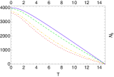
(a)  Number of condensate atoms in the lattice.

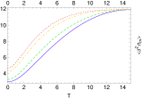
(b)  Atoms number fluctuations in a single site of the lattice.

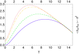
(c)  Correlations between close neighbours. Here, ${\textbf{m}}=(0,0,0)$ and ${\textbf{m}}^{\prime}=(1,0,0)$.

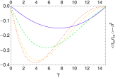
(d)  Correlations between distant neighbours. Here, ${\textbf{m}}=(0,0,0)$ and ${\textbf{m}}^{\prime}=(5,5,5)$.

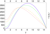
(e)  Momemtum modes correlations. Here, ${\textbf{k}}=(2,2,2).$

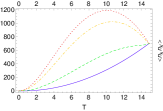
(f)  Momemtum modes correlations. Here, ${\textbf{k}}=(1,0,0)$ and ${\textbf{k}}^{\prime}=(1,1,1).$

Figure 6: (Color online) Statistical properties of the SF phase in an optical lattice. Here, $M=11\!\times\!11\!\times\!11$ and $N=3M$. Different colors of the curves refer to different values of the parameter $U$: blue (solid) for $U=0$, green (dashed) for $U=1$, yellow (dot-dashed) for $U=4$, red (dotted) for $U=6$. The selected values of $U$ imply the following values of quantum depletion: 0%, 1.6%, 6.8%, 9.7%, respectively. The strength of interaction $U$ and temperature $T$ are expressed in units of $J$.

Finally, by transforming to the position space with the help of Eqs. (36) and (37), we evaluate single-site occupation number statistics, i.e. single-site fluctuations, $\left\langle\delta^{2}n_{{\textbf{m}}}\right\rangle=\left\langle n_{{\textbf{m}}}^{2}\right\rangle-n^{2}$, and correlations, $\left\langle n_{{\textbf{m}}}n_{{\textbf{m}}^{\prime}}\right\rangle-n^{2}$, between each pair of sites in the lattice. At the final stage they are substituted into Eq. (26) determining the angular distribution of the scattered light.

In Fig. 6 we present results for the statistics of the SF state realized in an optical lattice. We have chosen four different values of the strength of interactions $U$ that correspond to quantum depletion ranging from $0$ to approximately $0.1$, which should be proper in the regime of a weakly interacting gas where the Bogoliubov method is applicable. An upper limit of temperatures we consider is established by the conditions of validity of the MD ensemble approximation that, for sufficiently large systems, works well up to a temperature close to the critical temperature $T_{C}$. As expected, we observe that the on-site fluctuations increase monotonically up to $T_{C}$. In contrast, the correlations between populations of different sites exhibit non-monotonic behavior that is strongly dependent on a distance between the considered sites. The phenomena can be understood by studying the behavior of these statistical quantities at small and at large temperatures. Readily, in the limit $T\rightarrow 0$ the on-site fluctuations and correlations follow the behavior presented in Section IV: $\left\langle\delta^{2}n_{{\textbf{m}}}\right\rangle=n-\frac{n^{2}}{N}$ and $\left\langle n_{{\textbf{m}}}n_{{\textbf{m}}^{\prime}}\right\rangle-n^{2}=-\frac{n^{2}}{N}$. On the contrary, at large temperatures the fluctuations and correlations can be described consistently within a model of $N$ indistinguishable particles distributed over $M$ degenerate levels: $\left\langle\delta^{2}n_{{\textbf{m}}}\right\rangle=n^{2}+n$ and $\left\langle n_{{\textbf{m}}}n_{{\textbf{m}}^{\prime}}\right\rangle-n^{2}=0$. For both of the limits, the analytical expressions are derived under the assumption $U/J\rightarrow 0$, however the approximations work reasonably well also for finite values of the ratio $U/J$. The last two panels of Fig. 6 present correlations between different modes in the momentum space. We note that the correlation between an excited and the condensate mode $\left\langle n_{{\textbf{k}}}n_{{\textbf{0}}}\right\rangle$, exhibits a maximum at some moderate temperature. This follows simply from the competition between the process of thermal depletion of the condensate and a growth of the thermal fraction. Similarly, in case of correlations between two excited modes, we observe that at some temperature the initial growth of $\left\langle n_{{\textbf{k}}}n_{{\textbf{k}}^{\prime}}\right\rangle$ is suppressed by decrease in population of these modes in favor of population of modes of some higher quasi-momentum.

V.3 Statistical properties of the Mott-insulator phase

We introduce grand canonical Bose-Hubbard Hamiltonian ${\cal K}$:

$${\cal K}=-J\!\!\!\!\sum\limits_{\left\langle{\textbf{m}},{\textbf{m}}^{\prime}\right\rangle}g^{\dagger}_{{\textbf{m}}}g_{{\textbf{m}}^{\prime}}+\frac{1}{2}U\!\sum\limits_{{\textbf{m}}}\hat{n}_{{\textbf{m}}}\left(\hat{n}_{{\textbf{m}}}-1\right)-\mu\sum_{{\textbf{m}}}\hat{n}_{{\textbf{m}}}.$$ (51)

In order to describe quantum statistics of the Mott insulator phase at finite temperatures we adopt a mean-field decoupling approximation Sachdev (1999); van Oosten et al. (2003). In analogy to the Bogoliubov approach, we introduce a complex mean-field parameter $\psi\equiv\left\langle g_{m}\right\rangle$ that can be physically interpreted as an order parameter that is nonzero if the system is superfluid. Below the phase transition point, the symmetry related to the gauge invariance of the phase is spontaneously broken and without losing generality we can assume that $\psi$ is real. The new parameter allows one to decouple the hopping term occurring in Eq. (51)

$$g^{\dagger}_{{\textbf{m}}}g_{{\textbf{m}}^{\prime}}=\psi\left(g^{\dagger}_{{\textbf{m}}}+g_{{\textbf{m}}^{\prime}}\right)-\psi^{2}.$$ (52)

By performing this substitution we can decompose Hamiltonian (51) into a sum of mean-field local Hamiltonians ${\cal K}^{\scriptscriptstyle{MF}}_{{\textbf{m}}}$: $\displaystyle{\cal K}=\sum_{{\textbf{m}}}{\cal K}^{\scriptscriptstyle{MF}}_{{\textbf{m}}}$, where

$${\cal K}^{\scriptscriptstyle{MF}}_{{\textbf{m}}}\equiv -2DJ\psi\left(g_{{\textbf{m}}}+g^{\dagger}_{{\textbf{m}}}\right)+2DJ\psi^{2}-\mu\hat{n}_{{\textbf{m}}}$$

$$+\frac{1}{2}U\hat{n}_{{\textbf{m}}}\left(\hat{n}_{{\textbf{m}}}-1\right).$$ (53)

At zero temperature, calculation of the ground-state energy and its minimization as a function of the superfluid order parameter $\psi$ yields the phase diagram analytically van Oosten et al. (2001). However, for non-zero temperatures the model has no analytical solution, and one has to resort to numerical calculations. Namely, by diagonalization of Eq. (53) we calculate grand canonical partition function $\mathcal{Z}(\psi)$,

$$\mathcal{Z}(\psi)=\textrm{Tr}\left\{e^{-\beta{\cal K}^{\scriptscriptstyle{MF}}_{{\textbf{m}}}}\right\},$$ (54)

and on its grounds we determine the grand thermodynamic potential $\Omega(\psi)$,

$$\Omega(\psi)=-\frac{1}{\beta}\ln\mathcal{Z}(\psi).$$ (55)

Subsequently, by minimizing $\Omega(\psi)$ with respect to $\psi$, we obtain the equilibrium value of the order parameter that we use to calculate all the relevant thermodynamic quantities. In particular:

$$\left\langle n_{{\textbf{m}}}(\mu)\right\rangle= \frac{1}{\mathcal{Z}}\textrm{Tr}\left\{\hat{n}_{{\textbf{m}}}e^{-\beta{\cal K}^{\scriptscriptstyle{MF}}_{{\textbf{m}}}}\right\},$$ (56)

$$\left\langle\delta^{2}n_{{\textbf{m}}}(\mu)\right\rangle= \frac{1}{\mathcal{Z}}\textrm{Tr}\left\{\hat{n}^{2}_{{\textbf{m}}}e^{-\beta{\cal K}^{\scriptscriptstyle{MF}}_{{\textbf{m}}}}\right\}-n^{2}.$$ (57)

In the homogeneous lattice $\left\langle n_{{\textbf{m}}}(\mu)\right\rangle=n$, and this identity is used to determine the value of the chemical potential, for a given single site occupation $n$.

Our mean-field approach assumes decoupling of different sites, $\left\langle n_{{\textbf{m}}}n_{{\textbf{m}}^{\prime}}\right\rangle-n^{2}=0$ (${\textbf{m}}\neq{\textbf{m}}^{\prime}$), that agrees with the zero temperature statistics of the MI assumed in section IV. This, in general, is not valid at higher temperatures when the hopping between adjacent sites in non-negligible. Nevertheless, it is satisfied at smaller temperatures considered here.

In Fig. 7 we present the mean single-site occupation and fluctuations as a function of the chemical potential, and for different system temperatures. The calculations have been performed within the mean-field model for $U/J=128$. One can see the existence of a characteristic temperature above which, the flat steps in $\left\langle n_{{\textbf{m}}}(\mu)\right\rangle$ disappear completely, and the curve becomes monotonically increasing. This crossover is accompanied by an appearance of nonzero fluctuations for all values of $\mu$ presented in the plot. This corresponds to the transition from the MI to the normal phase. In MI phase the system is infinitely compressible: $\partial\left\langle n\right\rangle/\partial\mu=0$, while in the normal or SF phase the compressibility becomes finite: $\partial\left\langle n\right\rangle/\partial\mu\neq 0$. Since the on-site fluctuations can be expressed as $\langle\delta^{2}n\rangle=\partial\left\langle n\right\rangle/\partial(\beta\mu)$, therefore they can be nonzero only in the normal or SF phase. In order to distinguish between the normal and SF phases one can resort to the value of the order parameter $\psi$. Finally, we note that our mean-field treatment neglects the effects of correlations between different sites and the quantum fluctuations. In the more accurate models that take these effects into account, the on-site fluctuations become nonzero already in the MI regime, close to the boundaries with the SF or normal phases.

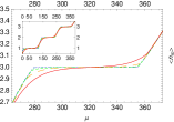
(a)  Average atoms number in a single site in the lattice.

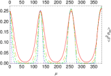
(b)  Atoms number fluctuations in a single site in the lattice.

Figure 7: (Color online) Statistical properties of Mott insulator phase for $U=128$. Colors of the curves refer to different values of temperature being considered: blue (dotted) for $T=0$, dark green (dot-dashed) for $T=4$, green (dashed) for $T=6$, orange (long-dashed) for $T=8$ and red (solid) for $T=11$. All the values of parameters are expressed in units of $J$.

VI Finite temperature scattering in three dimensions

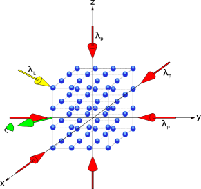
Figure 8: (Color online) Setup. A three-dimensional optical cubic lattice generated by lasers $\lambda_{p}$ (red arrows) is illuminated by a probing laser $\lambda_{L}$ (yellow arrow) set at angles $({\phi}_{L},{\theta}_{L})$. A detector of scattered photons (green arrow) is aligned in a direction $({\phi}_{d},{\theta}_{d})$.

We consider three-dimensional cubic lattice and assume a sufficiently large value of the trapping potential depth $V_{0}$ to neglect corrections from the nonlocal Franck-Condon factors. The setup is depicted in Fig. 8. The lasers creating an optical lattice ($\lambda_{p}$, red arrows) are set along $x,y$ and $z$ axes. In general, the position of a probing laser ($\lambda_{L}$, yellow arrow, characterized by angles $\phi_{L}$, $\theta_{L}$) and detector (green arrow, characterized by angles $\phi_{d}$, $\theta_{d}$) can be optimized in order to minimize the contribution from the classical component in the vicinity of the direction of the measurement, cf. Appendix B. This is of particular importance in case of large lattices for which, due to a big number of interference fringes, the detector would collect the photons from several interference peaks. Here, though, we do not choose the optimal configuration, we consider some example geometry which not only sufficiently reduces an influence of the classical component but also offers relatively simple experimental realization. Namely, we choose the direction of the probing beam along one of the diagonals of the lattice cube, ${\textbf{k}}_{L}=|{\textbf{k}}_{L}|(\frac{1}{\sqrt{3}},-\frac{1}{\sqrt{3}},\frac{1}{\sqrt{3}})$, and a detector centered around ${\textbf{k}}=|{\textbf{k}}_{L}|(\frac{1}{\sqrt{2}},-\frac{1}{\sqrt{2}},0)$.

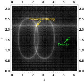
Figure 9: (Color online) Logarithm of the structure function $F({\textbf{q}})$ for MI phase at zero temperature, as a function of spherical angles of detection, $(\theta,\phi)$. The probing laser is set at $({\phi}_{L},{\theta}_{L})$. Bright regions correspond to directions in which a large number of photons is scattered. The yellow circle (pointed by the yellow arrow) indicates the direction of the probing laser (global maximum of number of scattered photons). The green circle (pointed by the green arrow) refers to the direction of a detection ${\textbf{k}}=|{\textbf{k}}_{L}|(\frac{1}{\sqrt{2}},-\frac{1}{\sqrt{2}},0)$ which is discussed in details in the text. Here, $M=55$, $N=3M$ and $V_{0}=20E_{r}$.

In analogy to the one-dimensional case, we expect that sharp differences in the intensity of light scattered from the SF and MI phases can be observed at angles for which the classical component $F^{clas}(\phi,\theta)$ is negligible. In Fig. 9 we present the zero-temperature structure function $F(\phi,\theta)$ for MI phase that is equivalent to the $F^{clas}(\phi,\theta)$. Keeping in mind that the quantum component $F^{quant}(\phi,\theta)$ for the SF state is slowly varying and of order of $N$, we observe that $({\phi}_{d},{\theta}_{d})$ is indeed a promising direction for a measurement that can distinguish the two quantum phases. In Fig. 10 we corroborate this observation by presenting scattering patterns for the superfluid $F^{SF}(\phi,\theta)$ and Mott-insulator $F^{MI}(\phi,\theta)$ phases at $T=0$. The plots show cross-sections of $F(\phi,\theta)$ along the planes of constant $\theta$ and $\phi$, respectively. Evidently, for the specific values of parameters we have chosen and for the assumed directions of the probing laser and of the detector, the difference of number of photons scattered from the SF and MI phases is of order $N\sim 10^{5}$ and thus should be readily measurable in experiment.

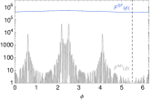
(a)   $F(\phi,\theta=\theta_{d})$

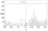
(b)   $F(\phi=\phi_{d},\theta)$

Figure 10: (Color online) Zero-temperature $F^{SF}(\theta,\phi)$ (top blue curves) and $F^{MI}(\theta,\phi)$ (bottom gray curves) with domains restricted to $\phi$ (left figure) and $\theta$ (right figure). The position of the photons detector $({\phi}_{d},{\theta}_{d})$ is indicated with vertical dashed lines. Here, $M=55\!\times\!55\!\times\!55$, $N=3M$, $\lambda_{p}/\lambda_{L}=1$ and $V_{0}=20E_{r}$.

We turn now to the thermal effects and their influence on the angular distribution of scattered photons. Analyzing Fig. 11 and Fig. 12 we observe the isotropic and monotonic growth of the intensity of scattered light with temperature, for both SF and MI phases. In the case of SF phase, this behavior can be explained on the grounds of the Eq. (26) rewritten in the momentum representation by means of transformation (36)-(37). In particular, if we disregard anomalous averages while calculating expectation values of the form $\left\langle a^{\dagger}_{{\textbf{k}}_{1}}a_{{\textbf{k}}_{2}}a^{\dagger}_{{\textbf{k}}_{3}}a_{{\textbf{k}}_{4}}\right\rangle$, i.e. if we perform the approximation

$$\left\langle a^{\dagger}_{{\textbf{k}}_{1}}a_{{\textbf{k}}_{2}}a^{\dagger}_{{\textbf{k}}_{3}}a_{{\textbf{k}}_{4}}\right\rangle \approx\delta_{{\textbf{k}}_{1},{\textbf{k}}_{2}}\delta_{{\textbf{k}}_{3},{\textbf{k}}_{4}}\left\langle a^{\dagger}_{{\textbf{k}}_{1}}a_{{\textbf{k}}_{1}}a^{\dagger}_{{\textbf{k}}_{2}}a_{{\textbf{k}}_{2}}\right\rangle$$

$$\phantom{\simeq}+\delta_{{\textbf{k}}_{1},{\textbf{k}}_{4}}\delta_{{\textbf{k}}_{2},{\textbf{k}}_{3}}\left\langle a^{\dagger}_{{\textbf{k}}_{1}}a_{{\textbf{k}}_{2}}a^{\dagger}_{{\textbf{k}}_{2}}a_{{\textbf{k}}_{1}}\right\rangle,$$ (58)

Eq. (26) can be rewritten as:

$$F({\textbf{q}})= \frac{1}{M^{2}}\left|f_{\textbf{0},\textbf{0}}({\textbf{q}})\right|^{2}\!\Biggl{[}N(N-1)\left|\sum\limits_{{\textbf{m}}}e^{\imath{\textbf{q}}{\textbf{r}}_{{\textbf{m}}}}\right|^{2}$$

$$+\sum_{{\textbf{k}}\neq{\textbf{k}}^{\prime}}\left\langle n_{{\textbf{k}}}n_{{\textbf{k}}^{\prime}}\right\rangle\left|\sum\limits_{{\textbf{m}}}e^{\imath\left(-{\textbf{k}}+{\textbf{k}}^{\prime}+{\textbf{q}}\right){\textbf{r}}_{{\textbf{m}}}}\right|^{2}\Biggr{]}$$

$$+N\left|f_{\textbf{0},\textbf{0}}({\textbf{q}})\right|^{2}.$$ (59)

When temperature increases, a number of particles occupying excited modes grows (see Fig. 6), causing an increase in correlations terms $\left\langle n_{{\textbf{k}}}n_{{\textbf{k}}^{\prime}}\right\rangle$. In consequence, the total intensity of the scattered light $F^{SF}(T)$ increases monotonically with temperature in any direction of measurement. We note that some correlations terms $\left\langle n_{{\textbf{k}}}n_{{\textbf{k}}^{\prime}}\right\rangle$ start to decrease above some characteristic temperature (see Fig. 6). However this does not influence the total structure function $F^{SF}(T)$ that grows monotonically with $T$.

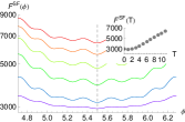
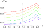
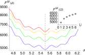
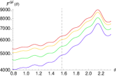
Figure 11: (Color online) Structure function $F(\phi,\theta)$ for SF phase of bosons in a three-dimensional optical lattice. The preferred position of the detector $({\phi}_{d},{\theta}_{d})$ is marked with vertical dashed lines. The plots show the cross sections along the constant $\theta$ (left panels) and constant $\phi$ (right panels). The calculations have been performed for ${}^{87}\textrm{Rb}$ atoms, $\lambda_{p}=\lambda_{L}=850\textrm{nm}$, $M=11\!\times\!11\!\times\!11$ and $N=3M$. The upper panels show results for constant $V_{0}=6.80E_{r}\hskip 1.9919pt(U=4)$ and increasing value of temperature: $T=0,3,5,7,9,11$ (ordered from the bottommost to the topmost curve) with $U$ and $T$ being expressed in units of $J$. The bottom panels show results for constant temperature $T=10$ and increasing value of trapping potential depth: $V_{0}=3.66E_{r}\hskip 1.9919pt(U=1),V_{0}=5.15E_{r}\hskip 1.9919pt(U=2),V_{0}=6.80E_{r}\hskip 1.9919pt(U=4),V_{0}=7.82E_{r}\hskip 1.9919pt(U=6)$, ordered from the bottommost to the topmost curve. The insets show the number of photons scattered in the direction of a detector $({\phi}_{d},{\theta}_{d})$ versus temperature (top panel) and interaction strength (bottom panel).

Similarly, an increase in the interaction strength (an increase in the lattice potential depth, equivalently) results in larger population of excited modes, partially due to increase in the quantum depletion. This behavior leads to a growth of the correlation terms in Eq. (59) and again to the monotonic increase in the full function $F^{SF}(U)$.

In the case of MI phase, presented in Fig. 12, the increase in the number of scattered photons $F^{MI}(T)$ is fully determined by a temperature-driven growth of single-site fluctuations that have been presented in Fig. 7.

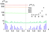
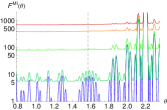
Figure 12: (Color online) Structure function $F(\phi,\theta)$ for MI phase of bosons in a three-dimensional optical lattice. The preferred position of the detector $({\phi}_{d},{\theta}_{d})$ is marked with vertical dashed lines. The plots show the cross sections along the constant $\theta$ (left panels) and constant $\phi$ (right panels). The calculations have been performed for ${}^{87}\textrm{Rb}$ atoms, $\lambda_{p}=\lambda_{L}=850\textrm{nm}$, $M=55\!\times\!55\!\times\!55$, $N=3M$, $V_{0}=18.3E_{r}\;(U=128)$, $\mu=320$ and temperatures: $T=0,6,8,10,11$ (ordered from the bottommost to the topmost curve), with $U,T$ and $\mu$ being expressed in units of $J$. The inset shows the number of photons scattered in the direction of a detector $({\phi}_{d},{\theta}_{d})$ versus temperature.

VII Summary and conclusions

We have investigated the scattering of a weak and far-detuned laser light from a system of ultracold bosons in an optical lattice. We have shown that the light scattering can be used as a probe of the on-site quantum statistics, in particular fluctuations and correlations. Calculating the statistics for the superfluid and Mott-insulator phases at finite temperatures, we have determined the angular distributions of the mean number of the scattered photons. The profiles of the scattered light are fully determined by the on-site particle number fluctuations and correlations and thus allow for an experimental verification of the present theoretical models describing the statistics in ultracold gases. For the 3D optical lattice we have determined the optimal geometry at which the contribution from the Bragg scattering pattern is minimized. We have shown that even at some non-optimal configurations, which can be more accessible from the experimental point of view, this contribution is sufficiently small and allows one to measure the effects of quantum statistics. Our main conclusion is that by careful choice of the measurement geometry one can distinguish between different phases, even at finite temperatures, and observe the effects of the finite temperature statistics of a Bose gas.

Appendix A Corrections for weak lattice potentials due to the nonlocal Franck-Condon coefficients

By applying the local approximation in the derivation of Eq. (26) we have neglected contributions from the nonlocal Franck-Condon coefficients. Here, we calculate the leading contribution from the neglected nearest-neighbor terms.

In the case of the MI phase the expression is proportional to $N$:

$$\Delta F^{MI}({\textbf{q}})=\left(|f_{1,0}({\textbf{q}})|^{2}+|f_{\textrm{-}1,0}({\textbf{q}})|^{2}\right)\left(1+n\right)N.$$ (60)

Although it scales the same as the difference between MI and SF phase, the coefficients $f_{1,0}({\textbf{q}})$ and $f_{\textrm{-}1,0}({\textbf{q}})$ rapidly tend to zero with the increasing lattice depth.

Similarly, the nearest neighbor correction for superfluid state reads

$$\Delta F^{SF}({\textbf{q}}) =\Big{(}|f_{1,0}({\textbf{q}})|^{2}+|f_{\textrm{-}1,0}({\textbf{q}})|^{2}$$

$$\phantom{=}\,+2\textrm{Re}\!\left\{f_{1,0}^{\ast}({\textbf{q}})\,f_{\textrm{-}1,0}({\textbf{q}})\right\}\Big{)}$$

$$\phantom{=}\times\left[N+n^{2}\left(1-\frac{1}{N}\right)\left|\sum\limits_{n}e^{\imath{\textbf{q}}{\textbf{r}}_{n}}\right|^{2}\right].$$ (61)

A brief estimate leads to

$$\Delta F^{SF}({\textbf{q}})\approx\left(|f_{1,0}({\textbf{q}})|^{2}+|f_{\textrm{-}1,0}({\textbf{q}})|^{2}\right)N,$$

that, again, contains small coefficients $f_{1,0}({\textbf{q}})$ and $f_{\textrm{-}1,0}({\textbf{q}})$ rapidly decreasing with the lattice potential depth.

Appendix B Optimization of positions of a probing laser and a detector in the 3D case

In this appendix we derive the condition for optimal configuration of the probing light and of the photon detector, which lead to the minimal contribution from the classical amplitude of the scattered light. We start with the classical part of the structure function $F({\textbf{q}})$, defined in (28)

$$F^{clas}({\textbf{q}}) =n^{2}\left|f_{\textbf{0},\textbf{0}}({\textbf{q}})\right|^{2}\left|\sum\limits_{{\textbf{m}}}e^{\imath{\textbf{q}}{\textbf{r}}_{{\textbf{m}}}}\right|^{2}.$$ (62)

The label m, enumerates lattice sites: $r_{\textbf{m}}=d(\hat{{\textbf{x}}}m_{x}+\hat{{\textbf{y}}}m_{y}+\hat{{\textbf{z}}}m_{z})$, with integer $m_{x},m_{y},m_{z}$. For a simple cubic lattice the summation can be easily performed

$$F^{clas}({\textbf{q}})=n^{2}\left|f_{\textbf{0},\textbf{0}}({\textbf{q}})\right|^{2}\prod_{i=x,y,z}\frac{\sin^{2}\left(\frac{M}{2}q_{i}d\right)}{\sin^{2}\left(\frac{1}{2}q_{i}d\right)}.$$ (63)

For the rest of the derivation we introduce a convenient parametrization of the vectors ${\textbf{k}}_{L}=k_{L}(\alpha_{x},\alpha_{y},\alpha_{z})$, ${\textbf{k}}=k_{L}(\beta_{x},\beta_{y},\beta_{z})$, and ${\textbf{q}}=k_{L}(\eta_{x},\eta_{y},\eta_{z})$ describing the momenta of the incoming and scattered photons, and the momentum transfer, respectively. The dimensionless numbers $\eta_{i}$, $\alpha_{i}$, and $\beta_{i}$ satisfy: $|\eta_{i}|<2$, $|\alpha_{i}|<1$, and $|\beta_{i}|<1$ for $i=x,y,z$. Expressing the translation vector of the lattice and the wave vector of the laser in terms of the wavelengths: $d=\lambda_{p}/2$ and $k_{L}=2\pi/\lambda_{L}$, we rewrite Eq. (63) in the following way

$$F^{clas}({\textbf{q}})=n^{2}\left|f_{\textbf{0},\textbf{0}}({\textbf{q}})\right|^{2}\prod_{i=x,y,z}\frac{\sin^{2}\left(M\frac{\pi}{2}\eta_{i}\frac{\lambda_{p}}{\lambda_{L}}\right)}{\sin^{2}\left(\frac{\pi}{2}\eta_{i}\frac{\lambda_{p}}{\lambda_{L}}\right)}.$$ (64)

Typically, the angular dependence of the Franck-Condon factor $\left|f_{\textbf{0},\textbf{0}}({\textbf{q}})\right|^{2}$ is rather weak, which follows from the fact that the characteristic size of a single lattice site, given by a harmonic oscillator length associated with the potential well, is much smaller than the wavelength of the probing laser. In such conditions the scattering due to $\left|f_{\textbf{0},\textbf{0}}({\textbf{q}})\right|^{2}$ is almost isotropic, and most of the angular dependence is determined by the interference term characteristic for the Bragg scattering. The function $\sin^{2}(Mx)/\sin^{2}(x)$ generating the interference pattern, takes the maxima at $x=n\pi$, while the minimal amplitude of oscillations occurs in the middle between two neighboring maxima: $x=\pi(n+\frac{1}{2})$. In fact, the latter determines the desired condition for the measurement with the minimal contribution from the classical component: $\eta_{i}\frac{\lambda_{p}}{\lambda_{L}}=1+2n_{i}$, where $n_{i}$ are integers, and $i=x,y,z$. For simplicity we further consider only the simplest case $\lambda_{p}=\lambda_{L}$. Since $|\eta_{i}|<2$, the only possibility is $\eta_{i}=\pm 1$, which leads to the following three conditions:

$$\beta_{j}-\alpha_{j}=\pm 1,\qquad\textrm{for }j=x,y,z.$$ (65)

The other two conditions are given by the conservation of the momenta of the scattered photons: $|{\textbf{k}}|=|{\textbf{k}_{L}}|=k_{L}$, which results in

$$|\alpha_{x}|^{2}+|\alpha_{y}|^{2}+|\alpha_{z}|^{2}=|\beta_{x}|^{2}+|\beta_{y}|^{2}+|\beta_{z}|^{2}=1.$$ (66)

By combining (65) and (66), we obtain the following two equations determining the coordinates of k and ${\textbf{k}}_{L}$:

$$|\alpha_{x}|^{2}+|\alpha_{y}|^{2}+|\alpha_{z}|^{2}=1,$$ (67)

$$|\alpha_{x}\pm 1|^{2}+|\alpha_{y}\pm 1|^{2}+|\alpha_{z}\pm 1|^{2}=1.$$ (68)

Readily, there are infinitely many solutions of the two above equations. All of them lie on a circle that is a common part of two spheres in the three-dimensional space. One of the possible solutions is given by the set of numbers: ${\textbf{k}}_{L}=k_{L}\left(6-\sqrt{6},6-\sqrt{6},6+2\sqrt{6}\right)/12$ and ${\textbf{k}}=k_{L}\left(-6-\sqrt{6},-6-\sqrt{6},2\sqrt{6}-6\right)/12$.

Finally, we note that for the optimal geometry determined by Eqs. (67) and (68), an average of the classical component $F^{clas}({\textbf{q}})$ over a finite solid angle containing several interference peaks results in the three-dimensional analog of formula (32)

$$\overline{F^{clas}({\textbf{q}})}=\left|f_{{\textbf{0}},{\textbf{0}}}({\textbf{q}})\right|^{2}\frac{n^{2}}{8}.$$ (69)

Here, we have applied the condition $\sin\left(\frac{1}{2}q_{i}d\right)=1$ that follows the conditions for the optimal choice of the measurement geometry. We stress that this result is derived for this particular geometry, and only in this case the sine squared factors average out to $\frac{1}{2}$ independently in all three directions.

References

• Dalfovo et al. (1999) F. Dalfovo, S. Giorgini, L. P. Pitaevskii, and S. Stringari, Rev. Mod. Phys. 71, 463 (1999).
• Giorgini et al. (2008) S. Giorgini, L. P. Pitaevskii, and S. Stringari, Rev. Mod. Phys. 80, 1215 (2008).
• Bloch et al. (2008) I. Bloch, J. Dalibard, and W. Zwerger, Rev. Mod. Phys. 80, 885 (2008).
• Idziaszek et al. (2009) Z. Idziaszek, L. Zawitkowski, M. Gajda, and K. Rzazewski, Europhys. Lett. 86, 10002 (2009).
• Chuu et al. (2005) C.-S. Chuu, F. Schreck, T. P. Meyrath, J. L. Hanssen, G. N. Price, and M. G. Raizen, Phys. Rev. Lett. 95, 260403 (2005).
• et al. (2007) J. et al., Nature 445, 402 (2007).
• (7) R. Bucker, A. Perrin, S. Manz, T. Betz, C. Koller, T. Plisson, J. Rottmann, T. Schumm, and J. Schmiedmayer, URL http://arxiv.org/abs/0907.0674.
• Lewenstein and You (1993) M. Lewenstein and L. You, Phys. Rev. Lett. 71, 1339 (1993).
• Javanainen and Ruostekoski (1995) J. Javanainen and J. Ruostekoski, Phys. Rev. A 52, 3033 (1995).
• Saito and Ueda (1999) H. Saito and M. Ueda, Phys. Rev. A 60, 3990 (1999).
• Moore and Meystre (1999) M. G. Moore and P. Meystre, Phys. Rev. Lett. 83, 5202 (1999).
• Zhang et al. (1999) W. Zhang, C. A. Sackett, and R. G. Hulet, Phys. Rev. A 60, 504 (1999).
• Ruostekoski (1999) J. Ruostekoski, Phys. Rev. A 60, R1775 (1999).
• Törmä and Zoller (2000) P. Törmä and P. Zoller, Phys. Rev. Lett. 85, 487 (2000).
• Wong et al. (2000) T. Wong, O. Müstecaplıoḡlu, L. You, and M. Lewenstein, Phys. Rev. A 62, 033608 (2000).
• Mekhov et al. (2007a) I. B. Mekhov, C. Maschler, and H. Ritsch, Phys. Rev. Lett. 98, 100402 (2007a).
• Mekhov et al. (2007b) I. B. Mekhov, C. Maschler, and H. Ritsch, Nat. Phys. 3, 319 (2007b).
• Chen et al. (2007) W. Chen, D. Meiser, and P. Meystre, Phys. Rev. A 75, 023812 (2007).
• Eckert et al. (2007) K. Eckert, O. Romero-Isart, M. Rodriguez, M. Lewenstein, E. S. Polzik, and A. Sanpera, Nat. Phys. 4, 50 (2007).
• Sadler et al. (2007) L. E. Sadler, J. M. Higbie, S. R. Leslie, M. Vengalattore, and D. M. Stamper-Kurn, Phys. Rev. Lett. 98, 110401 (2007).
• Idziaszek et al. (2000) Z. Idziaszek, K. Rza̧żewski, and M. Lewenstein, Phys. Rev. A 61, 053608 (2000).
• Mekhov et al. (2007c) I. B. Mekhov, C. Maschler, and H. Ritsch, Phys. Rev. A 76, 053618 (2007c).
• Lewenstein et al. (1994) M. Lewenstein, L. You, J. Cooper, and K. Burnett, Phys. Rev. A 50, 2207 (1994).
• Van Hove (1954) L. Van Hove, Phys. Rev. 95, 249 (1954).
• rem (a) We note that $S({\textbf{q}})$ is frequently defined in the literature as the Fourier transform of density fluctuations $S({\textbf{q}})=N^{-1}\int\!\!d^{3}x\!\!\int\!\!d^{3}y\>e^{\imath{\textbf{q}}\left({\textbf{x}}-{\textbf{y}}\right)}\left\langle\hat{\rho}({\textbf{x}})\hat{\rho}({\textbf{y}})\right\rangle-\left\langle\hat{\rho}({\textbf{x}})\right\rangle\left\langle\hat{\rho}({\textbf{y}})\right\rangle$ Pitaevskii and Stringari (2003).
• Pitaevskii and Stringari (2003) L. Pitaevskii and S. Stringari, Bose–Einstein Condensation (Oxford University Press, Oxford, 2003).
• Uys and Meystre (2008) H. Uys and P. Meystre, Phys. Rev. A 77, 063614 (2008).
• Gajda et al. (1996) M. Gajda, P. Krekora, and J. Mostowski, Phys. Rev. A 54, 928 (1996).
• Fisher et al. (1989) M. P. A. Fisher, P. B. Weichman, G. Grinstein, and D. S. Fisher, Phys. Rev. B 40, 546 (1989).
• Jaksch et al. (1998) D. Jaksch, C. Bruder, J. I. Cirac, C. W. Gardiner, and P. Zoller, Phys. Rev. Lett. 81, 3108 (1998).
• rem (b) $\lfloor x\rfloor$ denotes the greatest integer less than or equal to x.
• Bogoliubov (1947) N. Bogoliubov, J. Phys. USSR 11, 23 (1947).
• van Oosten et al. (2001) D. van Oosten, P. van der Straten, and H. T. C. Stoof, Phys. Rev. A 63, 053601 (2001).
• Svidzinsky and Scully (2006) A. A. Svidzinsky and M. O. Scully, Phys. Rev. Lett. 97, 190402 (2006).
• Navez et al. (1997) P. Navez, D. Bitouk, M. Gajda, Z. Idziaszek, and K. Rza̧żewski, Phys. Rev. Lett. 79, 1789 (1997).
• Grossmann and Holthaus (1997) S. Grossmann and M. Holthaus, Opt. Express 1, 262 (1997).
• Weiss and Wilkens (1997) C. Weiss and M. Wilkens, Opt. Express 1, 272 (1997).
• Sachdev (1999) S. Sachdev, Quantum Phase Transitions (Cambridge University Press, 1999).
• van Oosten et al. (2003) D. van Oosten, P. van der Straten, and H. T. C. Stoof, Phys. Rev. A 67, 033606 (2003).