Cobordisms of Free Knots and Gauss Words

Abstract

We investigate cobordisms of free knots. Free knots and links are also called homotopy classes of Gauss words and phrases. We define a new strong invariant of free knots which allows to detect free knots not cobordant to the trivial one.

1 Introduction

The aim of the present work is to consider cobordisms of free knots. Free knots and links [Ma] (also called homotopy classes of Gauss words and phrases, see [Tu, Gib]) are a substantial simplification of homotopy classes of curves on $2$-surfaces, and at the same time, a simplification of virtual knots and links, introduced by Kauffman in [Ka].

A conjecture due to Turaev [Tu] stating that all free knots are trivial was solved very recently independently by Manturov [Ma] and Gibson [Gib].

We consider cobordism classes of free knots and give a strong invariant which allows to detect free knots not cobordant to the trivial one.

2 Basic Definitions

We shall encode free knots and links by using framed graphs.

Throughout the paper by a four-valent graph we mean the following generalization: a finite $1$-complex $\Gamma$ with each connected component being homeomorphic either to a circle or to a four-valent graph; by a vertex of a four-valent graph we mean only vertices of those components which are homeomorphic to four-valent graphs, and by edges we mean both edges of four-valent graphs and circular components (the latter will be called cyclic edges).

We call a four-valent graph framed if for every vertex of it a way of splitting of the four incident half-edges into two pairs is indicated. Half-edges belonging to the same pair are to be called opposite. We shall also use the term opposite with respect to edges containing opposite half-edges.

By an isomorphism of framed $4$-graphs we always mean a framing-preserving homeomorphism.

By a unicursal component of a framed four-valent graph we mean either its connected component homeomorphic to the circle or an equivalence class of edges of some non-circular component, where the equivalence is generated by the opposite relation.

Let $K$ be a framed four-valent graph, and let $X$ be a vertex of $X$. Let $(a,c)$ and $(b,d)$ be the two pairs of opposite half-edges of the graph $K$ at $X$. By smoothings of $K$ at $X$ we call two framed four-valent graphs obtained from $K$ by deleting $X$ and reconnecting the adjacent (non-opposite) edges: for one graph we connect the pairs $(a,b)$ and $(c,d)$, and for the other graph we connect $(a,d)$ and $(b,c)$.

Consider a chord diagram $C$. Then the corresponding framed four-valent graph $G(C)$ with a unique unicursal component is constructed as follows. With the chord diagram having no chords one associates the graph $G_{0}$ consisting of a unique circular component. Otherwise the edges of the graph are in one-to-one correspondence with arcs of the chord diagrams, and vertices are in one-to-one correspondence with chords.

Those arcs which are incident to the same chord end, correspond to formally opposite half-edges.

The first Reidemeister move for four-valent framed graphs is an addition/removal of a loop, see Fig. 1.

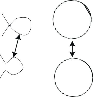
Figure 1: The First Reidemeister Move and Its Chord Diagram Version

The second Reidemeister move is an addition/removal of a bigon, formed by a pair of edges, which are adjacent (not opposite) to each other at each of the two vertices, see Fig. 2.

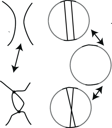
Figure 2: The Second Reidemeister Move and Its Chord Diagram Version

The third Reidemeister move is shown in Fig. 3.

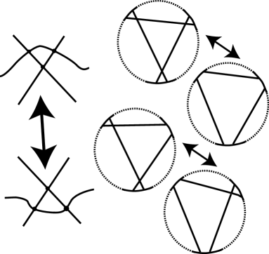
Figure 3: The Third Reidemeister Move and Its Chord Diagram Version

• 2.1. A free link is an equivalence class of framed four-valent graphs modulo Reidemeister moves. Obviously, the number of components of a framed four-valent graph does not change under Reidemeister moves, thus, one can talk about the number of components of a framed links. A free knot is a $1$-component free link.

  Free knots can be treated as equivalence classes of corresponding Gauss diagrams (chord diagrams) modulo corresponding moves on Gauss diagrams (which mimic the moves on four-valent framed graphs). Analogously, for free-links one can introduce Gauss diagrams on several circles which stand for different components of the link, and chord ends may belong to different circles.

  Here a chord diagram (Gauss diagram) on one circle is a split collection of unordered pairs of distinct points on a circle $S^{0}_{1}\sqcup\dots\sqcup S^{0}_{k}\subset S^{1}$. The circle $S^{1}$ is here called the cycle of the chord diagram.

  Every pair of points $S_{i}^{0}$ is called a chord and points from this pair are called chord ends. We call two chords $S_{i}^{0},S_{j}^{0}$ linked if the chord ends $S_{i}^{0}$ belong to different connected components of $S^{1}\backslash S_{j}^{0}$.

  A chord is even if the number of chords linked with it, is even, and odd otherwise.

By an even symmetric configuration $C$ on a chord diagram $D$ we mean a set of pairwise disjoint segments $C_{i}$ on the cycle of the chord diagram which possess the following properties:

1) the ends of the segments do not coincide with chord ends;

2) the number of chords inside any segment is finite;

3) the number of endpoints of chords inside any segment is even;

4) every chord having one endpoint in $C$ has the other endpoint in $C$.

5) Consider the involution $i$ of the cycle which fixes all points outside the segments $C_{i}$ and reflects all segments along the radii. This involution naturally defines new points to be chord ends, and thus defines the new chord diagram $i(D)$.

We require that the configuration $C$ is symmetric, i. e., chord diagrams $D$ and $i(D)$ are equal.

Note that if a chord has two endpoints in different segments $C_{i}$ and $C_{j}$ then it is not self-symmetric.

By an elementary cobordism we mean a transformation of a chord diagram deleting all chords belonging to the even symmetric configuration, as well as the inverse transformation.

We say that two Gauss diagrams are cobordant if one can be obtained from the other by a sequence of elementary cobordisms and third Reidemeister moves.

• 2.1. The first two Reidemeister moves are partial cases of elementary cobordisms, unlike the third Reidemeister move.

Since the first two Reidemeister moves are partial cases of elementary cobordisms, it makes sense to talk about cobordism classes of free knots, not only cobordism classes of Gauss diagrams.

• 2.2. The definition of cobordisms given above agrees with the definition of word cobordism (nanoword cobordism) [Tu]. With each (cyclic) double occurrence word in some given alphabet one associates a Gauss diagram, and words which are cobordant in Turaev’s sense yield cobordant diagrams. However, nanowords usually correspond to Gauss diagrams with some decoration (labeling) of chords, and the notion of elementary cobordism usually requires some conditions imposed on chords belonging to the symmetric configuration.

  In this sense, cobordism classes of free knots are the simplest variant of cobordism classes of nanowords. Nevertheless, we show that there are free knots which are not cobordant to zero.

The main result of the present paper is to prove the existence of (in fact, infinitely many) free knots which are not cobordant to zero.

To prove this problem, we shall construct a cobordism invariant for free knots.

3 The Mapping $\Delta$ and Its Iterations

Let $K$ be a framed four-valent graph. Each unicursal component $K_{i}$ of $K$ can be treated as a four-valent framed graph with a Gauss diagram $D_{i}$. Thus, some vertices of the graph $K$ can be represented by chords of one of $D_{i}$’s (namely, those vertices lying on one unicursal component). Among these, let us choose even vertices (in the sense of the Gauss diagram $D_{i}$), and at each even vertex $X$ of $K$, we consider the smoothing $K_{X}$ (one of the two possible) for which the number of unicursal components is greater than that of $K$ by $1$.

Now let ${\cal G}$ be the set of ${\mathbb{Z}}_{2}$-linear combinations of equivalence classes of framed four-valent graphs modulo second and third Reidemeister moves.

Set $\Delta(K)=\sum\limits_{X}K_{X}\in{\cal G}$, where the sum is taken over all crossings $X$ of $K$.

Then the following statement holds.

Statement 3.1.

The map $\Delta$ is a well defined map from ${\cal G}$ to ${\cal G}$.

Proof.

Indeed, assume $K$ is obtained from $K^{\prime}$ by a third Reidemeister move. Consider the three crossings $a_{1},a_{2},a_{3}$ of $K$ involved in this move, and the corresponding crossings $a^{\prime}_{1},a^{\prime}_{2},a^{\prime}_{3}$ of $K^{\prime}$. By construction, $a_{i}$ lies in one unicursal component of $K$ if and only if $a^{\prime}_{i}$ lies in one unicursal component of $K^{\prime}$. Moreover, $a$ is even if and only if $a^{\prime}_{i}$ is even.

It is now easy to see that whenever $a_{i}$ is even, the smoothing $K_{a_{i}}$ gives the same impact to ${\cal G}$ as that of $K^{\prime}_{a^{\prime}_{i}}$ (the corresponding framed 4-valent graphs are either isomorphic or differ by a second Reidemeister move).

Now, if $K$ and $K^{\prime}$ differ by a second Reidemeister move and $K^{\prime}$ has two more crossings $a,b$ in comparison with $K$, then it obviously follows that either both crossings $a$, $b$ are even or none of them is even. In the first case, the summands in $\Delta(K)$ are in one-to-one correspondence with those in $\Delta(K^{\prime})$ and the corresponding diagrams in each pair differ by a second Reidemeister move. If both $a$ and $b$ are odd, then it is obvious that the smoothings at these crossings give equal impact to $K^{\prime}$, and since we are working over ${\mathbb{Z}}_{2}$, they cancel each other. ∎

Consequently, if we take $\Delta$ $k$ times, the resulting map $\Delta^{k}$ is also invariant.

So, if $K$ and $K^{\prime}$ are two framed four-valent graphs which are obtained from each other by a third Reidemeister move, then for every positive integer $k$ we have $\Delta^{k}(K^{\prime})=\Delta^{k}(K)$.

4 The map $\Gamma$

Let $L$ be a framed four-valent graph with $k$ unicursal components. With $L$ we associate a graph $\Gamma(L)$ (not necessarily four-valent, but without loops and multiple edges) and a number $I(L)$ according to the following rule.

The graph $\Gamma(L)$ will have $k$ vertices which are in one-to-one correspondence with unicursal components of $L$. Two vertices are connected by an edge if and only if the corresponding components share an odd number of points.

The following statement is evident.

Statement 4.1.

If two framed four-valent graphs $L$ and $L^{\prime}$ are homotopic then $\Gamma(L)=\Gamma(L^{\prime})$.

Now, we define the number $j(L)$ from the graph $\Gamma(L)$ in the following way.

If $\Gamma(L)$ is not connected we set $j(L)=0$, otherwise $j(L)$ is set to be the number of edges of $\Gamma(L)$.

5 The invariant

Fix a natural number $n$.

Let $\cal G$ be a linear space generated over ${\mathbb{Z}}_{2}$ by formal vectors $\{a_{i}\},i\in\mathbb{N}$.

Let $K$ be a framed four-valent graph with one unicursal component, and let $\Delta^{n}(K)$ be the corresponding linear combination of four-valent graphs.

For a four-valent framed graph $L$, we set $I(L)=a_{j(L)}$ if $j(L)\neq 0$ and $I(L)=0$ otherwise. We extend this map to ${\mathbb{Z}}_{2}$–linear combinations of framed four-valent graphs by linearity.

Now, set

$$\mathop{\kern 0.0pt\operator@font I}\nolimits^{(n)}(K)=I(\Delta^{n}(K)).$$

The main result of the paper is the following

Theorem 5.1.

If $K$ and $K^{\prime}$ are cobordant then $\mathop{\kern 0.0pt\operator@font I}\nolimits^{(n)}(K)=\mathop{\kern 0.0pt\operator@font I}\nolimits^{(n)}(K^{\prime})$.

The proof of this theorem follows from two statements. By virtue of Statement 4.1, the mapping $\mathop{\kern 0.0pt\operator@font I}\nolimits^{(n)}(\cdot)$ is invariant with respect to the third Reidemeister move (since so is $\Delta^{n}$).

Moreover, the following statement holds

Statement 5.1.

If $K_{2}$ is obtained from $K_{1}$ by an elementary cobordisms (removal of an even symmetric configuration), then $\mathop{\kern 0.0pt\operator@font I}\nolimits^{(n)}(K_{1})=\mathop{\kern 0.0pt\operator@font I}\nolimits^{(n)}(K_{2})$

Having proved Statement 5.1, we shall get Theorem 5.1. Indeed, it will follow that $\mathop{\kern 0.0pt\operator@font I}\nolimits^{(n)}$ is invariant under all elementary cobordisms and third Reidemeister moves, hence, under arbitrary cobordisms.

We will prove Statement 5.1 in the last section of our paper

6 An example

• Consider the free knot $K$ represented by the Gauss diagram shown in Fig 4. Let us calculate $\mathop{\kern 0.0pt\operator@font I}\nolimits^{(3)}(K)$. We have:

  $$\Delta(\raisebox{-0.25pt}{\includegraphics[width=19.91684pt]{chord.eps}})=\raisebox{-0.25pt}{\includegraphics[width=46.94687pt]{chord1_1.eps}}+\raisebox{-0.25pt}{\includegraphics[width=46.94687pt]{chord1_2.eps}}+\raisebox{-0.25pt}{\includegraphics[width=46.94687pt]{chord1_3.eps}},$$

  $$\Delta^{2}(\raisebox{-0.25pt}{\includegraphics[width=19.91684pt]{chord.eps}})=\Delta(\raisebox{-0.25pt}{\includegraphics[width=46.94687pt]{chord1_1.eps}})+\Delta(\raisebox{-0.25pt}{\includegraphics[width=46.94687pt]{chord1_2.eps}})+\Delta(\raisebox{-0.25pt}{\includegraphics[width=46.94687pt]{chord1_3.eps}})$$

  $$=\raisebox{-0.4pt}{\includegraphics[width=46.94687pt]{chord2_1.eps}}+\raisebox{-0.4pt}{\includegraphics[width=46.94687pt]{chord2_2.eps}}+\raisebox{-0.4pt}{\includegraphics[width=46.94687pt]{chord2_3.eps}}+\raisebox{-0.4pt}{\includegraphics[width=46.94687pt]{chord2_4.eps}}+\raisebox{-0.4pt}{\includegraphics[width=46.94687pt]{chord2_5.eps}}+\raisebox{-0.4pt}{\includegraphics[width=46.94687pt]{chord2_6.eps}},$$

  $$\Delta^{3}(\raisebox{-0.25pt}{\includegraphics[width=19.91684pt]{chord.eps}})=\Delta(\raisebox{-0.4pt}{\includegraphics[width=46.94687pt]{chord2_1.eps}})+\Delta(\raisebox{-0.4pt}{\includegraphics[width=46.94687pt]{chord2_2.eps}})+\Delta(\raisebox{-0.4pt}{\includegraphics[width=46.94687pt]{chord2_3.eps}})$$

  $$+\Delta(\raisebox{-0.4pt}{\includegraphics[width=46.94687pt]{chord2_4.eps}})+\Delta(\raisebox{-0.4pt}{\includegraphics[width=46.94687pt]{chord2_5.eps}})+\Delta(\raisebox{-0.4pt}{\includegraphics[width=46.94687pt]{chord2_6.eps}})$$

  $$=\raisebox{-0.4pt}{\includegraphics[width=46.94687pt]{chord3_1.eps}}+\raisebox{-0.4pt}{\includegraphics[width=46.94687pt]{chord3_2.eps}}+\raisebox{-0.4pt}{\includegraphics[width=46.94687pt]{chord3_3.eps}}+\raisebox{-0.4pt}{\includegraphics[width=46.94687pt]{chord3_4.eps}}+\raisebox{-0.4pt}{\includegraphics[width=46.94687pt]{chord3_5.eps}}+\raisebox{-0.4pt}{\includegraphics[width=46.94687pt]{chord3_6.eps}}$$

  $$=\raisebox{-0.4pt}{\includegraphics[width=46.94687pt]{chord3_1.eps}}+\raisebox{-0.4pt}{\includegraphics[width=46.94687pt]{chord3_2.eps}}.$$

  Thus, applying $\Delta^{3}$ we get $\mathop{\kern 0.0pt\operator@font I}\nolimits^{(3)}(K)=a_{4}$.

  Thus, by Theorem 5.1, the cobordism class of $K$ is non-trivial.

Figure 4: The Gauss diagram of a free knot not cobordant to the unknot

Obviously, there are infinitely many such examples. We shall construct them and discuss the cobordism group of free knots as well as further invariants in a separate publication

7 Sketch of the Proof of Statement 5.1

Let $K_{2}$ be the Gauss diagram obtained from a Gauss diagram $K_{1}$ by deleting an even symmetric configuration ${\tilde{K}}$.

The chords of $K_{1}$ belong to three sets:

1. the set of those chords which corresponding to chords of $K_{2}$, we denote them for both $K_{1}$ and $K_{2}$ by $\gamma_{j}$’s.

2. the set of those chords $\beta_{j}$ which are fixed under the involution $i$ on ${\tilde{K}}$,

3. the set of pairs of chords $\alpha_{k}$ and ${\bar{\alpha}}_{k}=i(\alpha_{k})$ which are obtained from each other by the involution $i$ (here ${\bar{\bar{\alpha}}}_{k}=\alpha_{k}$).

Now, for every framed four-valent graph $L$, $\Delta^{n}(L)$ is a sum of some subsequent smoothings $\Delta^{(p_{1}\dots p_{k})}(L)$, where all $p_{i}$’s are vertices of $L$ where $p_{i}$ occurs to be even after smoothing all $p_{1},\dots,p_{i-1}$.

Now, $\Delta^{n}(K_{1})$ naturally splits into $3$ types of summands:

1. Those where all $p_{i}$ are some $\gamma_{j}$. These smoothings are in one-to one correspondence with smoothings of $K_{2}$. We claim that the corresponding elements $I(\Delta^{(p_{1}\dots p_{k})}(K_{1}))$ and $I(\Delta^{(p_{1}\dots p_{k})}(K_{2}))$ are equal.

2. Those where at least one of $p_{i}$ is $\beta_{j}$, and neither $\alpha$’s nor ${\bar{\alpha}}$’s occur among $p_{i}$. We claim that each of these summands $I(\Delta^{(p_{1}\dots p_{k})}(K_{1}))$ is zero.

3. Those summands where at least one of $p_{i}$’s is $\alpha_{j}$ or ${\bar{\alpha}}_{j}$.

These summands are naturally paired: the elements $I(\Delta^{(p_{1}\dots p_{k})}(K_{1}))$ and $I(\Delta^{({\bar{p}}_{1}\dots\bar{p}_{k})}(K_{1}))$ are equal.

Let us first prove 1. Since segments of our even symmetric configurations have no common points with chords $\gamma_{j}$, we see that after smoothing along any of $\gamma$’s, every segment will completely belong to one circle. This means that the corresponding graphs $\Gamma(\Delta^{(p_{1}\dots p_{k})}(K_{1}))$ and $\Gamma(\Delta^{(p_{1}\dots p_{k})}(K_{2}))$ are isomorphic.

Indeed, the vertices corresponding to $\beta$ do not change the graph at all, since every vertex corresponding to $\beta$ is an intersection of one component of $\Delta^{\dots}$ with itself.

Moreover, the vertices $X_{i}$ and $X^{\prime}_{i}$ corresponding to $\alpha_{i}$ and ${\bar{\alpha}}_{i}$ belong to the same pair of component, so their impact to the graph cancels.

To prove 2, let us take one $p_{j}=\beta_{k}$, and consider the segment $C_{i}$ of $K_{1}$ where $\beta_{k}$ lies.

Without loss of generality, we may assume that $\beta_{k}$ is the innermost chord in $K_{1}$ amongst those chords $p_{l}$ we use for smoothings.

Now, our summand looks like $\Delta^{\dots\beta_{k}\dots}$. Smoothing $K_{1}$ along $\beta_{k}$ cuts a free knot (component) which has ends only in the segment $C_{i}$. It is obvious that this unicursal component will be split in the sense of the graph $\Gamma$: it will have even intersection with any other unicursal component (since whenever it shares a vertex $X$ of some other component, this vertex necessarily corresponds either to some $\alpha$ (or to some ${\bar{\alpha}}$) and the corresponding ${\bar{\alpha}}$ (resp., $\alpha$) will be shared by the same two components).

The proof of 3 follows from one basic fact: the number of components of a $1$-manifold obtained from a chord diagram by smoothing some of its chords can be defined from the intersection graph of this chord diagram, see [Sob]. We shall give a rigorous proof of 3 in a separate publication.

The authors express their gratitude to V.P.Ilyutko for implementing a computer program calculating the invariant $\mathop{\kern 0.0pt\operator@font I}\nolimits$.

References

- [Gib] Gibson, A., Homotopy Invariants of Gauss Words, ArXiv:Math.GT/0902.0062.
- [Ka] L. H. Kauffman, Virtual knot theory, Eur. J. Combinatorics. 1999. V. 20, N. 7, pp. 662–690.
- [Ma] Manturov, V.O., On Free Knots, ArXiv:Math.GT/0901.2214
- [Sob] E. Soboleva, Vassiliev Knot Invariants Coming from Lie Algebras and -Invariants (2001), Journal of Knot Theory and Its Ramifications, 10 (1), pp. 161–169.
- [Tu] Turaev, V.G., Cobordisms of Words, Arxiv:Math.CO/0511513, v.2.