Brownian Dynamics of charged particles in a constant magnetic field
Abstract
Numerical algorithms are proposed for simulating the Brownian dynamics of charged particles in an external magnetic field, taking into account the Brownian motion of charged particles, damping effect and the effect of magnetic field self-consistently. Performance of these algorithms is tested in terms of their accuracy and long-time stability by using a three-dimensional Brownian oscillator model with constant magnetic field. Step-by-step recipes for implementing these algorithms are given in detail. It is expected that these algorithms can be directly used to study particle dynamics in various dispersed systems in the presence of a magnetic field, including polymer solutions, colloidal suspensions and, particularly complex (dusty) plasmas. The proposed algorithms can also be used as thermostat in the usual molecular dynamics simulation in the presence of magnetic field.
pacs:
52.40.Hf, 52.25.Vy, 05.40.-aI Introduction
Brownian Dynamics (BD) simulation method for many-body systems of particles immersed in a liquid, gaseous or plasma medium Ermak ; Allen ; vanGunsteren1982 ; Branka ; Chin ; Allen1989 ; Lemons1999 ; Lemons2002 can be regarded as a generalization of the usual Molecular Dynamics (MD) method for many-body systems in free space. While the MD method is based on Newton’s equations of motion, the BD method is based on their generalization in the form of Langevin equation and its integral Lemons2002 :
| (1) | |||||
where, as usual, , and are, respectively, the mass, velocity and position of a Brownian particle, whereas is a systematic (deterministic) force coming from external fields and/or from inter-particle interactions within the system. What is different from Newton’s equations is the appearances of dynamical friction, , and random, or Brownian acceleration, . These two force components represent two complementing effects of a single, sub-scale phenomenon: numerous, frequent collisions of the Brownian particle with molecules in the surrounding medium. While the friction represents an average effect of these collisions, the random acceleration represents fluctuations due to discreteness of collisions with molecules, and is generally assumed to be a delta-correlated Gaussian white noise. The friction and random acceleration are related through a fluctuation-dissipation theorem which includes the ambient temperature, therefore guaranteeing that a Brownian particle can ultimately reach thermal equilibrium within the medium Lemons2002 .
The Langevin equations, Eq. (1), can be numerically integrated in a manner similar to Newton’s equations in the MD simulation, which gives rise to several algorithms for performing BD simulation, such as the Euler-like Ermak , Beeman-like Allen ; Allen1989 , Verlet-like vanGunsteren1982 , and Gear-like Predictor-Corrector (PC) methods Hou2008pop , as well as a wide class of Runge-Kutta-like algorithms (see, e.g., Branka ; Chin ). All those methods were used successfully to study problems in various dispersed systems, such as polymer solutions Ottinger , colloidal suspensions Chen2004 and, in particular, complex (dusty) plasmas Hou2008pop ; Zheng1995 ; Hoffmann2000 ; Vaulina2002 ; Hou2006 ; Hou2009 .
Recently, there has been a growing interest in studying the dynamics of dust particles and dust clouds in both unmagnetized Donko2009 ; Mendonca1997 and magnetized dusty Amatucci2004 ; Sato2001 ; Kaw2002 ; Shukla2002 plasmas. The topics studied so far include, besides Brownian motion of a dust particle in an unmagnetized plasma Mendonca1997 , also the gyromotion of a single dust particle and rotations Amatucci2004 of dust clouds Sato2001 ; Kaw2002 ; Shukla2002 and clusters Juan1998 ; Konopka2000 ; Cheung2003 ; Carsternsen2009 in a magnetized plasma. There have also been several theoretical proposals for studying waves and collective dynamics Shukla2009 in such magnetized plasma systems, in which dust particles are fully magnetized Uchida2004 ; Jiang2007 ; Jiang2007pop ; Feldmann2008 ; Farokhi2009 . However, exploring those proposals in the laboratory does not seem to be quite feasible as yet, due to many constrains Uchida2004 ; Jiang2007 ; Jiang2007pop ; Farokhi2009 . Therefore, it is desirable to have algorithms for numerical experiments that can validate the existing theories, on one hand, and that can serve as a guide for future laboratory experiments, on the other hand. Since there are no such algorithms, to the best of our knowledge, we propose here a few new BD algorithms, which treat an external magnetic field in the simulation in a manner consistent with the Langevin dynamics, Eq. (1).
The manuscript is organized in the following fashion. In Sec. II, we present the general formula for a BD simulation with a constant magnetic field. Detailed implementations to the Euler-, Beeman- and Gear-like methods are given, respectively, in Sections III, IV, and V. Concluding remarks are contained in Sec. VII.
II General formula for BD simulations
The dynamics of a charged Brownian particle in a constant external magnetic field is described by introducing the Lorentz force in the Langevin equation Lemons1999 ; Lemons2002
| (2) |
where is the charge on the particle and is the speed of light in vacuum.
As usual, certain assumptions must be made about the deterministic force in order to construct a meaningful algorithm for a many-particle simulation from the above equation. A common approach Ermak ; Allen ; vanGunsteren1982 ; Allen1989 is to assume that is only an explicit function of time . Thus, a Taylor series of or, equivalently the deterministic acceleration, , can be written as
| (3) |
where represents the th-order time derivative of . There are various ways to derive formulas for conducting a BD simulation from the Langevin equation, Eq. (2), based on the above Taylor series. We shall adopt the strategy outlined in Refs. Ermak ; Allen ; vanGunsteren1982 ; Allen1989 , and more recently implemented in Refs. Lemons1999 ; Lemons2002 , as it is simple and straightforward, especially for readers with some simulation background but without much background, or interest in stochastic calculus.
The Langevin equations, Eq. (2), may be integrated analytically in a short time, based on an adopted truncation rule for the series in Eq. (3), thereby giving an updating formula for a BD simulation. (We note that detailed technique for integrating the Langevin equation is particularly well described in Refs. Lemons1999 ; Lemons2002 .) The resultant formulas are actually expressions for the two random variables, and , which, under the assumptions that the Brownian acceleration in Eq. (2) is a Gaussian white noise and that is constant, turn out to be normally distributed random variables, according to the normal linear transform theorem Lemons1999 ; Lemons2002 . Therefore, the Cartesian components of the velocity and position vectors for a Brownian particle can be expressed in terms of their respective means and variances
| (4) |
where takes values , and , and is a shorthand notation for the standard normal random variable having zero mean and unit variance, the so-called unit normal Lemons1999 ; Lemons2002 . The superscripts attached to the components of random vectors and , appearing in Eq. (4), indicate that those two sets of unit normals are associated, respectively, with the velocity and position of the Brownian particle. We note that the Cartesian components of the vector are mutually independent, as are the components of the vector , but the vectors and are correlated, as will be shown below.
We should emphasize the importance of Eq. (4) because it provides a general updating formula for the BD simulation and also enables substantial simplifications in the subsequent design of our algorithm. Now, solving the stochastic differential equation, Eq. (2), and obtaining the two random variables and , is simply reduced to determining the two sets of deterministic quantities, the means and variances of and , as well as their covariances, assuming an appropriate truncation scheme for the deterministic acceleration, Eq. (3). To simplify the notation, in the following we shall denote the velocity and position means, respectively, by and , and we shall use standard deviations instead of variances.
II.1 Variances and covariances
We begin with variances and covariances because they do not depend on the form of deterministic acceleration, .
It should be noted that random increments in the velocity do not depend explicitly on the magnetic field and are therefore isotropic. The corresponding variances are then given by , where
| (5) |
with being the Boltzmann constant and the temperature of the medium. [It should be noted that in an equilibrium between the Brownian particle and the medium, is also the kinetic temperature of the Brownian particle. However, Brownian particles may have kinetic temperature that is different from , which opens a possibility of simulating non-equilibrium processes by using the BD].
However, random displacements of the position do depend explicitly on the magnetic field and therefore are non-isotropic. Let us assume and define to be the gyrofrequency of a Brownian charged dust particle. Then, we have and , where and are, respectively, standard deviations of the position in the directions perpendicular and parallel to the external magnetic field Lemons1999 ; Lemons2002 . In particular, we find
| (6) |
Furthermore, we have covariances Lemons1999 ; Lemons2002 , most of which are zeros. The non-zero covariances are , , , and Lemons1999 ; Lemons2002 (here, we use the definition for the covariance of two random variables, and ). In particular, we obtain Lemons1999 ; Lemons2002
| (7) | |||||
We note that, when , i.e., , one has and , so that , recovering the results for systems without magnetic field Lemons2002 .
II.2 Mean values
Given the expression for in terms its Taylor series in Eq. (3), one can obtain the means and in a number of ways by integrating Eq. (2). For simplicity, we follow here Lemons’ methodology Lemons1999 ; Lemons2002 , in which Eq. (2) is reduced to a set of deterministic (ordinary) differential equations by taking expectation values of both sides
| (8) | |||||
and using the fact that the Brownian acceleration is a Gaussian white noise with mean .
Equation (8) can be integrated analytically by assuming that initial conditions , , , , , , , are known at . One ends up with
| (9) |
With the assumption , the matrices are given by
| (10) |
where
| (11) |
for , and
| (12) |
for .
It is interesting to note that the coefficients satisfy very simple recursive relations
| (13) |
A special yet important case would be that of , i.e. , and consequently and , so that becomes a diagonal matrix with the diagonal elements being and, Eq. (9) reads as Hou2008pop
| (14) |
Further, when , and reduce to the usual coefficients of a Taylor series.
II.3 General updating formula
With the variances, covariances and means known, the updating formula for a BD simulation can be further written in a compact form as Lemons1999 ; Lemons2002
| (15) |
where
| (16) |
and
| (17) |
The unit normal vectors and , besides each having statistically independent Cartesian components, are also by design statistically independent from each other, and may be generated by the Box-Muller method Box1958 on a computer.
As expected, when , and become diagonal matrices with their diagonal elements being and , respectively, in which case Eqs. (15) become
| (18) |
It is worthwhile to point out that the updating formulae, Eqs. (15) and (18), can be actually interpreted as a two-step algorithm: first, one calculates the means of the velocity and position at time , and secondly, one adds explicitly random displacements (ERDs) of velocity and position. This is very important in the sense that the first step is nothing more than solving deterministic Newton’s equations with damping, so in principle many algorithms suitable for the MD simulation (for example, the Verlet, Beeman and even multi-step PC algorithms Allen1989 ; Berendsen1986 ) can be used here. On the other hand, the second step is independent of the first one, and can always be performed at the end of the time step as a correction to the previous step.
However, Eqs. (9) and (14) are still not very suitable for computer simulations, because they involve high-order derivatives of acceleration, which are not directly accessible in simulations. Further assumptions must be made about , and different ways of handling that issue then result in different simulation methods, such as the Euler-like, Beeman-like, Verlet-like and Gear-like methods.
III Euler-like method
In the Euler-like method Ermak , it is assumed that , or = constant in the time interval . Under this assumption, the velocity and position means are, respectively, given by
| (19) |
where the subscript in Eq. (19) is added to indicate reference to the Euler-like method. The special case of zero magnetic field can be simplified to Ermak
| (20) |
The procedure for implementing the simulation by using Euler-like method is as follows:
(a) Evaluate Eq. (19) [or Eq. (20) in the case of zero magnetic field] for the means of velocity and
displacement, given the initial conditions ,
and at .
(b) Generate two independent random vectors, and , which follow the standard normal
distribution (this may be usually done by using the Box-Muller method Box1958 ),
and substitute them into Eq. (15) [or Eq. (18) in the case of zero magnetic field], along with the means obtained in the first step.
(c) After the above two steps, a force evaluation is done, which will provide an initial condition for , along
with the updated position and velocity, to be used in the next step.
IV The Beeman-like method
In the Beeman-like method Allen ; Allen1989 , one has
| (21) |
Note that, according to the Beeman algorithm Allen ; Allen1989 , terms through first order in , i.e., , are kept in the expression for , and terms through second order in , i.e., , are kept in .
However, the above expressions are not yet suitable for a one-step simulation method Berendsen1986 , as they contain derivatives of the acceleration, which have to be replaced by a finite difference formula in terms of , and . Thus, we obtain the schemes of the Beeman-like algorithm Allen ; Allen1989 ,
| (22) | |||||
| (23) |
where , , and
[Note that, here, matrix operations should be understood as direct element operations, e.g., .]
In the special case of zero magnetic field, Eqs. (23) and (22) can be simplified to Allen
| (24) | |||||
| (25) |
with
Implementation of the Beeman-like method is also based on Eq. (15), and the detailed simulation procedure
is listed in the following:
(a) Evaluate Eq. (22) [or Eq.(24)] for the mean of displacement, given the initial conditions
,
and at , and at time .
(b) Evaluate a new deterministic acceleration based on the new position obtained in the previous step.
(c) Evaluate Eq. (23) [or Eq.(25)] for the mean of velocity, given the initial conditions
and at , and at time , as well as the newly obtained acceleration
in the previous step. [Note that, if one uses a periodic boundary condition,
it should be applied before this step.]
(d) Generate two independent random vectors, and , which follow the standard normal
distribution, and substitute them into Eq. (15) along with the means
obtained in the steps (a) and (c).
(e) Apply periodic boundary condition again if using it.
As one can see, the difference compared to the Euler-like method, is that here one has to do the force evaluation after the position update, but before the velocity update, in every time step, and one has to store the force value of the last step to be used for . In addition, one needs to apply the periodic boundary condition twice.
Let us note that the Verlet-like method vanGunsteren1982 was based on similar assumptions for as the Beeman-like method, and it was proven Allen that the Verlet-like method is numerically equivalent to the Beeman-like method in the position, while the latter seems to have a better accuracy in the velocity. Therefore, extensions of the Verlet-like method are not presented here.
V Gear-like Predictor-Corrector method
A Gear-like Predictor-Corrector (PC) method for BD Hou2008pop can be constructed in a direct analogy with the Gear method for MD simulations. Our Gear-like method also includes three stages, namely, predicting, force evaluating, and correcting Allen1989 ; Berendsen1986 , as in the MD simulation, but the difference here is that one has to add explicit random displacements of velocity and position by using Eq. (15) at the end of time step to complete the BD simulation. The basic procedure goes as follows.
V.1 Predicting
In the predicting stage, one has
| (26) |
where the superscript indicates that these are quantities in the predicting stage. For simplicity, we have dropped in the above all derivatives of higher than the third order, but we note that extensions to higher orders are quite straightforward. One notices in Eq. (26) that we have used Eq. (9) for the means of position and velocity, instead of using Taylor series for position and velocity which usually provide a basis for implementing the Gear method in the MD simulation Berendsen1986 ; Allen1989 . In the case of zero magnetic field, one simply needs to replace the means of velocity and position given by Eq. (14), instead of Eq. (9). The rest of the algorithm (derivatives of the force) is essentially the same as in the MD.
V.2 Force evaluating
In the next step, the predicted position is used to obtain a new force, or deterministic acceleration , and a difference between the predicted acceleration and the new acceleration is calculated as
| (27) |
It can be seen that this step is exactly the same as the one normally used for the Gear method in MD Allen1989 ; Berendsen1986 .
V.3 Correcting
In the correcting stage, the above difference term is further used to correct all predicted positions and their ”derivatives”, thus giving
| (28) |
where
| (29) |
and the coefficients are given in the Table 1. Note that the table is simply a reproduction of those appearing in Refs. Allen1989 ; Berendsen1986 , and is given here for completeness. By using parameters in different columns of that table, one can achieve 3rd-, 4th-, and 5th-order (or 4-, 5- and 6-value) Allen1989 ; Berendsen1986 Gear-like algorithms for the BD simulation. Note that the first two equations in Eq. (28) are slightly different from those in the MD in order to restore the damping effect on deterministic acceleration, and to maintain consistence with the corresponding terms in Eq. (9) [or the first two equations in Eq. (26)] as well. In the case of zero magnetic field, one simply replaces and in Eq. (28) by and , respectively.
| 3th-order | 4th-order | 5th-order | |
|---|---|---|---|
| 1 | 1 | 1 | |
| 0 | |||
| 0 | 0 |
V.4 Adding explicitly random displacements (ERDs)
To complete the BD simulation, we have to use the updating formula, Eq. (15), to add ERDs of the velocity and position. It should be noted that now the corrected value and must be used, respectively, in the places of and in Eq. (15).
We summarize the basic steps for implementing the Gear-like PC method:
(a) Eq. (26) is used to calculate predicted values of the position, velocity, acceleration and its derivatives,
given the initial conditions, , , , ,
and , at . Note that, for the very first few steps of the simulation,
, and are undefined. The simplest way to get around this
issue is to simply set all of them to zero at the very first step, and their values then will be updated during subsequent
iterations. A better way would be to start the simulation by using a Runge-Kutta procedure for the first few steps
Berendsen1986 . However, neither of these alternatives will have any significant
effects on the results in real many-particle simulations.
(b) Evaluate new acceleration by using the predicted position , and calculate its
difference with the predicted value by using Eq. (27).
[Note that, if one uses periodic boundary condition, it should be applied before the force evaluation.]
(c) Correct the predicted values of the position, velocity, acceleration and its derivatives by using
Eq. (28).
(d) Generate two independent random vectors, and , which follow the standard normal
distribution, and substitute them into Eq. (15) together with the corrected values
and .
(e) Apply periodic boundary condition again if using it.
The above is a basic procedure for using the Gear-like PC method for the BD. One might have noticed that the formulas, as well as the simulation procedure, are quite similar to those used in the Gear method for the MD based on Newton’s equations Berendsen1986 ; Allen1989 , apart from our use of Eqs. (26) and (29) to express the velocity and position, as well as the addition of ERDs at the end of every time step. Also, when and , the Gear-like method goes over to the Gear method for MD simulation.
VI Testing the algorithms
In the above we have developed numerical algorithms for simulating Brownian dynamics of charged particles in an external magnetic field. But how accurate are they in describing the actual Brownian motion? To answer this question, we present in this section some simple computational examples as testing cases and compare the performances of different algorithms presented above. For simplicity, we shall occasionally denote the Euler-like, Beeman-like, Verlet-like and Gear-like methods by EL, BL, VL, and GL, respectively.
As the simplest test cases, one could adopt comparison of the numerical results with the analytical results for some simple model problems, such as the classical harmonic oscillator, which had been used extensively to test algorithms for the MD simulation (see for example Ref. Berendsen1986 and Venneri1987 for nice reviews). We follow here the same logic and employ the model of a three-dimensional (3D) Brownian-harmonic-oscillator (BHO) in an external magnetic field Jimenez2008 , for which the Langevin equation (2) is reduced to
| (30) |
Since the magnetic field is in the direction of the Cartesian coordinate system, two independent processes take place. In the direction, the magnetic field does not have any effect on Brownian motion, so the Brownian particle behaves like a one-dimensional stochastically-damped harmonic-oscillator Chandrasekhar1943 ; Lemons2002 , while in the directions perpendicular to the magnetic field, i.e., in the plane, Brownian motion is much more complicated because of the coupling between the motions in the and directions via magnetic field. It is curious to note that, although the analytical solution for a BHO without magnetic field had been known for well over a half of the century Chandrasekhar1943 , the problem of BHO in an external magnetic field has been solved analytically only very recently by Jiménez-Aquino et al.Jimenez2008 .
Of course, the dynamics a BHO in magnetic field can be also traced by using the above described numerical methods. It is important to realize that, although the physical model for a BHO in magnetic field, Eq. (30), involves a very simple deterministic acceleration which depends on the particle’s position, it nevertheless provides a good test for our assumption that this acceleration depends on time only, and to examine the effects of various truncation schemes for the Taylor series representation of this acceleration, i. e., Eq. (3). The results of our numerical simulations of the BHO in a magnetic filed will be compared with the corresponding explicit analytical solutions, for which we refer the reader to the original reference Jimenez2008 . By doing so, one can evaluate the accuracy and performance of the numerical methods and validate the assumptions made in their derivation. The results will serve as a basic reference for future simulations of more complicated systems, such as magnetized dusty plasmas Venneri1987 .
According to the above discussion, and particularly referring to Eq. (15), the task of a BD simulation is simply to predict the position and velocity of a Brownian particle at time , given the set of initial conditions at time . Since and can be obtained numerically in two-steps, first, by calculating the means of the velocity and position at time and, second, by adding the ERDs of velocity and position, the performance of a BD simulation will be examined by testing the accuracy of both steps. We begin by testing the first step, i.e., calculating the means.
VI.1 Inaccuracy in calculating the means
Without any loss of generality, here and in the subsequent simulations we set , and , and choose the initial conditions to be , , and .
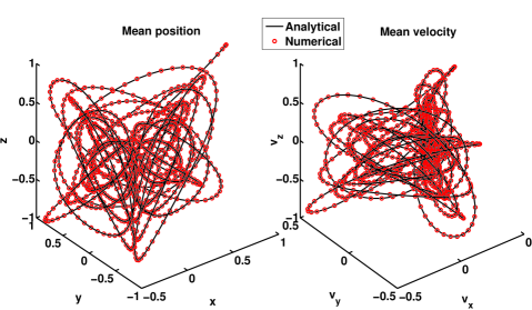
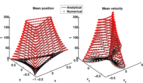
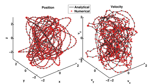
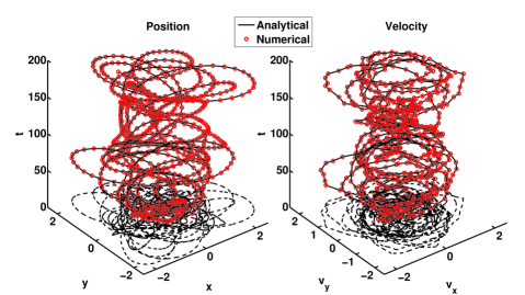
We first present in Fig. 1 examples of full 3D trajectories of the mean position and velocity for a BHO in time units, with , and the time step size . Solid lines are the results of the analytical solutions [Eqs. (B23)-(B34) in Jimenez2008 ], while the circles are numerical results calculated by using the GL-5 method. One might be particularly interested in the motion in the directions perpendicular to the magnetic field, which is shown in Fig. 2 as the time evolutions of the mean position and the mean velocity in the plane. We have found that details in the trajectory patterns strongly depend on the initial conditions and on the values of and , but the general tendency in trajectories is the same. Without Brownian acceleration, the initial energy of the oscillator would be sooner or later consumed by the damping, and the oscillator would come to rest at after long enough time. One sees from Figs. 1 and 2 that the numerical results agree very well with the analytical solutions. Good visual agreements were also found with numerical results of the GL-4, GL-3 and BL. However, quantitatively, they are quite different, as is shown in the following.
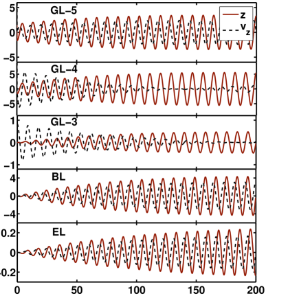
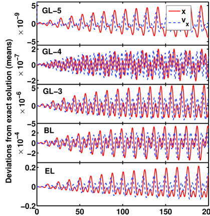
Figures 3 and 4 display deviations (differences) of the numerical results for the means of the position and velocity from the corresponding analytical results Jimenez2008 in time units, under the same conditions as in Fig. 1. Only deviations in the and directions are shown in Figs. 3 and 4, respectively, as those in the direction are essentially the same as those for , apart from a phase shift. The oscillatory patterns of deviations in the position and velocity approximately resemble those of the full solutions in Fig. 1, but they have much smaller amplitudes. One can observe the differences in magnitude of deviations for different methods, with the GL-5 method having the smallest deviations and therefore highest accuracy in both the and directions, while the EL method exhibits the largest deviations, as can be expected from our previous comparisons of these methods. It should also be noted that the performance of these methods is different in the and directions. One sees generally higher accuracy in the direction for the Gear-like methods, while the BL and EL methods have similar accuracies in the two directions. This indicates that the presence of the magnetic field also affects the accuracy of the computation.
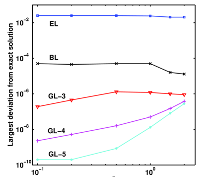
A more detailed analysis of the dependence of the accuracy on the magnitude of magnetic field is shown in Fig. 5, where the largest deviations of the position in the direction from the corresponding analytical solution Jimenez2008 are recorded in the first time units (which is a convention for the measure of accuracy Berendsen1986 ; Allen1989 ) and are plotted versus for different methods. One observes that, with the increase of the magnetic field intensity, the largest deviation of the EL method remains almost constant, while that of the BL method initially stays constant, but drops slightly when . The tendency observed in the Gear-like methods is the opposite. The initially excellent accuracy deteriorates with increasing magnetic field. The one with the highest accuracy, i.e., the GL-5 method is affected the most, as is shown. A similar scaling rule applies to simulations with other time steps and damping rates, as discussed next.
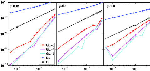
We make comparisons involving different time steps because that is always a key issue in both the MD and BD simulations. Fig. 6 shows the largest deviations (defined by the largest deviation in the first 20 units) of the position in the direction versus the size of the time step for different methods and different friction coefficients . This figure is plotted in a double logarithmic scale, and the curves are nearly straight lines. The slope of these lines is called the apparent order Berendsen1986 , illustrating the dependence of the error on the time step size. Namely, if the error is found to be proportional to , then the exponent is the apparent order. It is found that for very small , for example , as shown in Fig. 6, the apparent orders are , , , and , respectively for the Euler-like, Beeman-like, 3rd-, 4th-, and 5th-order Gear-like methods. These values are very close to those from the MD simulations where damping is absent Berendsen1986 , which proves the consistency of our computation. When increases, the absolute value of the error for Euler-like and Beeman-like methods decreases, while and remain almost unchanged. On the other hand, , and slightly decrease with increasing . For example, for , as shown in Fig. 6, the Gear-like methods have the worst performance in accuracy: their apparent orders become now , and ), but the magnitudes of their errors are still much smaller than those of the Beeman-like and Euler-like methods.
All the above tests show that the numerical methods, especially the Gear-like methods and Beeman-like method, can describe the mean values of the movement of a BHO with sufficiently high accuracy.
VI.2 Total inaccuracy
The tests carried out in this sub-section are similar to those in the previous one, but with the addition of the ERDs in both the position and velocity. We first show in Fig. 7 full trajectories of the BHO in time units, under the same condition as in Fig. 1. Again, solid lines show results of the analytical solutions Jimenez2008 , while circles are the numerical results calculated by using the GL-5 method. Motion of the BHO in the plane under the influence of magnetic field is shown in Fig. 8. One observes in both figures that the numerical results of the GL-5 method again agree very well with the analytical results.
Before giving a more quantitative analysis of the full deviations including the ERDs by using different methods, we comment on the accuracy in variances and covariances, Eqs. (6) and (7), which will help to better understand the deviations in full trajectories. In deriving Eqs. (6) and (7), we used the assumption that the deterministic force is an explicit function of time only, and we truncated the Taylor series representation for that force. However, in many realistic problems and in the models such as the BHO, the deterministic force depends explicitly on the particle position only. While we have seen in the previous sub-section that this assumption can provide a sufficiently accurate description of the means of the position and velocity for a BHO, a question remains as to how does this assumption affect the calculation of variances and covariances, i.e. the explicitly random part of displacements.
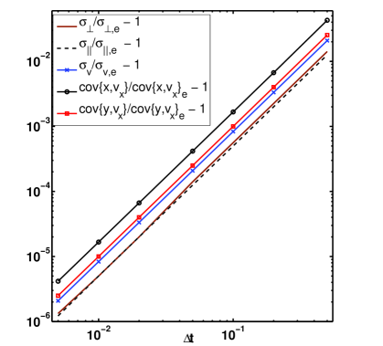
This is addressed in Fig. 9 which depicts relative deviations of the variances and covariances computed by the GL-5 method from the corresponding analytical results [Eqs. (26)-(34) in Jimenez2008 ] versus the time step size for and . (Note that, in the specific case of zero magnetic field, the analytical results of Jimenez2008 are identical to those of Refs. Chandrasekhar1943 ; Lemons2002 .) All deviations are seen to increase in Fig. 9 with increasing . In the log-log scale, all results form a cluster of parallel straight lines with a slope of about , indicating an apparent order of approximately . Judging by both the magnitude of deviations and by the apparent order, the accuracy for variances and covariances displayed in Fig. 9 is much lower than the accuracy for the means shown in Fig. 6. One would expect that the total accuracy of an algorithm will be largely determined by the accuracy of that part of the algorithm which has the lowest accuracy.
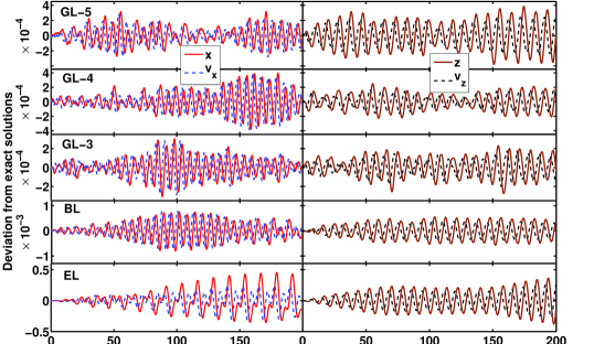
As before, we next carry out simulations over certain periods and record full deviations (means plus ERDs) of the position and velocity from the corresponding analytical results Jimenez2008 . All results are assembled in Fig. 10 for different methods in time units, with , and . One sees that, for all Gear-like methods the amplitude of the full deviation is about , which coincides with the corresponding deviation of cov{} shown in Fig. 9. This indicates that, for the Gear-like methods, the errors in calculation come mainly from the evaluation of variances and covariances, that is, from the addition of the ERDs. On the other hand, for the Beeman-like method and particularly for the Euler-like method, the magnitudes of the full deviations are larger than those of the deviations of variances and covariances shown in Fig. 9. This implies that the errors introduced by addition of the ERDs might have been amplified during the calculation of the means. All in all, the dramatic differences in deviations in the and directions seen between different methods in Figs. 3, 4 and 5 have disappeared when ERDs are added.
From now on, we shall examine mostly the behavior of simulations by monitoring the quantity
| (31) |
where and , which is defined to be proportional to the total energy of the Brownian oscillator at time and, as such, it contains inaccuracies in both the position and velocity. Note that, because of coupling with the medium through damping and Brownian acceleration, this energy is no longer a conserved quantity. In order to examine the energy conservation performance of our numerical methods, we normalize by its “exact” counterpart , which is simply obtained from Eq. (31) by substituting the explicit analytical expressions for the position and velocity Jimenez2008 . The resultant ratio should be then a conserved quantity in a simulation with the expected value of unity.
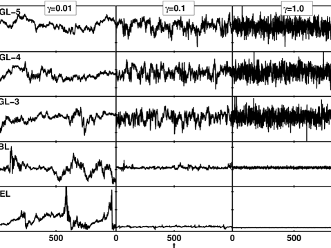
Figure 11 displays the relative deviation of energy from its exact counterpart Jimenez2008 , i.e., , calculated by using different methods for several damping rates, with and . To check the long time stability of these methods, a longer time scale of time units is adopted here. One sees that, for the Gear-like methods, the amplitude of deviation is quite similar to that of the position and velocity in Fig. 10. Also, the amplitude does not change appreciably with the damping rate, although the frequency of the noise changes dramatically as the collision frequency, i.e., the damping rate, increases from to . However, the situation for the Beeman-like and Euler-like methods is quite different. For the former, the amplitude of the deviation is approximately one order higher than that of the Gear-like methods at , but it decreases dramatically when increases, and reaches almost the same level as that of the Gear-like methods at about . For the latter, the amplitude of the deviation is about at , and is therefore comparable to the value of energy itself, indicating that this method is not stable under these conditions. However, it also decreases with increasing damping rate. So, it is obvious that finite damping actually stabilizes Beeman-like and Euler-like methods. This is not surprising at all, because the damping could also diminish errors inherited from a previous step during simulation. Indeed, previous studies Izaguirre2001 have demonstrated a possibility of stabilizing the MD simulation by introducing a small, but finite damping.
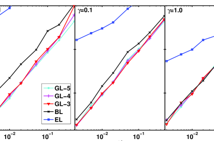
A more quantitative analysis of these results is shown in Fig. 12, in which the largest deviations in energy during time units are plotted versus the time step size for different values. One can see that the deviation of the Euler-like method is always the highest, but it decreases with increasing . Its magnitude suggests that this method should only be used for simulating systems with damping rate larger than and with very small time steps. As for the Gear-like methods, judging from the magnitude of deviations and the apparent order of around , their accuracy has reached the limit determined by the accuracy of deviations in variances and covariances shown in Fig. 9. Therefore, their deviations in the energy remain very close to each other, and they are nearly independent of . The performance of the Beeman-like method is in between the Euler-like and Gear-like methods for very small , but it reaches the same level as the Gear-like methods for large damping rates, such as .
VII Conclusions
We have presented several new algorithms for studying Brownian dynamics of charged particles in an external magnetic field. All these methods were tested by comparison with the available analytical results for a three-dimensional, Brownian-harmonic-oscillator model in the presence of an external magnetic field Jimenez2008 . It was found that the Gear-like method generally has the best performance in terms of accuracy, long time stability, and energy drift in a wide range of damping rates, and especially in the low-damping limit. Therefore, the Gear-like method should be highly recommended when studying systems with very low-damping and/or when using the BD method as a thermostat Ceriotti2009 in a MD simulation. The Beeman-like method can also cover a wide range of damping rates with reasonably good accuracy and with negligible energy drift. It should be recommended for simulating systems with intermediate damping rates. The Euler-like method, as can be expected, has the poorest performance and can be used with confidence only in simulating over-damped systems, such as colloidal suspensions and/or polymeric fluids. Further detailed tests based on applications to magnetized complex plasmas will be presented elsewhere Comingup .
We note that, besides applications in plasma physics, our numerical method could be also of interest in numerical studies of some stochastic processes in statistical physics Jimenez2008 ; Jimenez2008b ; Jimenez ; Jayannavar2007 ; Roy2008 , since we have actually tested here the recently developed analytical model for a Brownian-harmonic-oscillator in the presence of a magnetic field.
Acknowledgements.
L.J.H. acknowledges support from Alexander von Humboldt Foundation. Work at CAU is supported by DFG within SFB-TR24/A2. Z.L.M. acknowledges support from NSERC.References
- (1) D. L. Ermak, J. Chem. Phys. 62 (1975) 4189; D. L. Ermak, and H. Buckholz, J. Comput. Phys. 35, 169 (1980).
- (2) M. P. Allen, Mol. Phys. 40, 1073 (1980); 47, 599 (1982).
- (3) W. F. van Gunsteren, and H. J. C. Berendsen, Mol. Phys. 45, 637 (1982).
- (4) A. C. Brańka, and D. M. Heyes, Phys. Rev. E 58, 2611 (1998); 60, 2381 (1999).
- (5) S. A. Chin, Nucl. Phys. B 9, 498 (1989); Phys. Rev. A 42, 6991 (1990); Phys. Rev. E 73, 026705 (2006).
- (6) M. P. Allen and D. J. Tildesley, Computer Simulation of Liquids (Oxford University Press, New York, 1989).
- (7) D. S. Lemons and D. L. Kaufman, IEEE Trans. Plasma Sci. 27, 1288 (1999).
- (8) D. S. Lemons, An Introduction to Stochastic Processes in Physics (The Johns Hopkins University Press, Baltimore, 2002).
- (9) H. C. Öttinger, Stochastic Processes in Polymeric Fluids ( Springer, Berlin 1996).
- (10) J. C. Chen and A. S. Kim, Adv. Colloid Interface Sci. 112, 159 (2004).
- (11) X. H. Zheng and J. C. Earnshaw, Phys. Rev. Lett. 75, 4214 (1995).
- (12) G. P. Hoffmann, and H. Löwen, J. Phys.: Condens. Matter 12, 7359 (2000).
- (13) O. S. Vaulina and S. V. Vladimirov, Phys. Plasmas 9, 835 (2002).
- (14) L. J. Hou, Z. L. Mišković, K. Jiang, and Y. N. Wang, Phys. Rev. Lett. 96, 255005 (2006).
- (15) L. J. Hou, and A. Piel, Phys. Plasmas 15, 073707 (2008); J. Phys. A: Math. Theor., in press.
- (16) L. J. Hou, A. Piel, and P. K. Shukla, Phys. Rev. Lett. 102, 085002 (2009).
- (17) Z. Donkó, J. Goree, P. Hartmann, and B. Liu, Phys. Rev. E 79, 026401 (2009)
- (18) J. T. Mendonça, and P. K. Shukla, A. M. Martins, and R. Guerra, Phys. Plasmas 4, 674 (1997).
- (19) W. E. Amatucci, D. N. Walker, G. Gatling, and E. E. Scime, Phys. Plasmas 11, 2097 (2004).
- (20) N. Sato, G. Uchida, T. Kaneko, S. Shimizu, and S. Iizuka, Phys. Plasmas 8, 1786 (2001).
- (21) P. K. Kaw, K. Nishikawa, and N. Sato, Phys. Plasmas 9, 387 (2002).
- (22) P. K. Shukla, Phys. Lett. A 299, 258 (2002).
- (23) W. T. Juan, Z. H. Huang, J. W. Hsu, Y. J. Lai, and L. I, Chin, Phys. Rev. E 58, R6947 (1998); W. T. Juan, J. W. Hsu, Z. H. Huang, Y. J. Lai, and L. I, Chin. J. Phys. I37, 184 (1999).
- (24) U. Konopka, D. Samsonov, A. V. Ivlev, J. Goree, and V. Steinberg, Phys. Rev. E 61, 1890 (2000).
- (25) F. M. H. Cheung, A. A. Samarian, and B. W. James, New J. Phys. 5, 75 (2003).
- (26) J. Carstensen, F. Greiner, L. J. Hou, H. Maurer and A. Piel, Phys. Plasmas 16, 013702 (2009).
- (27) P. K. Shukla and B. Eliasson, Rev. Mod. Phys. 81, 25 (2009).
- (28) G. Uchida, U. Konopka, and G. Morfill, Phys. Rev. Lett. 93, 155002 (2004).
- (29) K. Jiang, L. J. Hou, X. Xu, and Y. N. Wang, New. J. Phys. 9, 57 (2007).
- (30) K. Jiang, Y. H. Song, and Y. N. Wang, Phys. Plasmas 14, 103708 (2007).
- (31) J. D. Feldmann, G. J. Kalman, P. Hartmann, and M. Rosenberg, Phys. Rev. Lett. 100, 085001(2008).
- (32) B. Farokhi, M. Shahmansouri and P. K. Shukla, ”Dust grain oscillations in 2D hexagonal dusty plasma crystals in the presence of a magnetic field”, submitted to Phys. Plasmas.
- (33) G. E. P. Box, and M. E. Muller, Ann. Math. Stat. 29, 610 (1958).
- (34) H. J. C. Berendsen and W. F. van Gunsteren, in Molecular-Dynamics Simulation of Statistical-Mechanical Systems (eds. G. Ciccotti and W. G. Hoover, North-Holland Physics Publishing, 1986).
- (35) G. D. Venneri and W. G. Hoover, J. Comput. Phys. 73, 468 (1987).
- (36) S. Chandrasekhar, Rev. Mod. Phys. 15, 1 (1943).
- (37) M. Ceriotti, G. Bussi, and M. Parrinello, Phys. Rev. Lett. 102, 020601 (2009).
- (38) J. A. Izaguirre, D. P. Catarello, J. M. Wozniak, and R. D. Skeel, J. Chem. Phys. 114, 2090 (2001).
- (39) L. J. Hou, P. K. Shukla, A. Piel, and , Z. L. Mišković, ”Wave spectra of 2D Yukawa solids and liquids with a perpendicular magnetic field”, to be submitted to Phys. Plasmas.
- (40) J. I. Jiménez-Aquino, R. M. Velasco, and F. J. Uribe, Phys. Rev. E 77, 051105 (2008).
- (41) J. I. Jiménez-Aquino, R. M. Velasco, and F. J. Uribe, Phys. Rev. E 77, 032102 (2008).
- (42) J. I. Jiménez-Aquino, and M. Romero-Bastida, Phys. Rev. E 74, 041117 (2006); 76, 021106 (2007).
- (43) A. M. Jayannavar and Mamata Sahoo, Phys. Rev. E 75, 032102 (2007).
- (44) D. Roy and N. Kumar, Phys. Rev. E 78, 052102 (2008).