Numerical Evaluation of Feynman Integrals by a Direct Computation Method

Abstract:

A purely numerical method, Direct Computation Method is applied to evaluate Feynman integrals. This method is based on the combination of an efficient numerical integration and an efficient extrapolation. In addition, high-precision arithmetic and parallelization technique can be used in this method if required. We present the recent progress in development of this method and show results such as one-loop 5-point and two-loop 3-point integrals.

1 Introduction

This paper describes a computational method for the loop integrals. This method is named as Direct Computation Method and its advantage is handling singularities in a purely numerical way which appear in the denominator of the integrand . We have already computed several diagrams with one-loop and two-loop such as

• One-loop vertex and box diagrams with/
  without infrared divergence[1, 2, 3, 4],

• Two-loop planar and non-planar vertex
  diagram[5].

In this paper, we present the brief description of this method and show another examples of loop integrals.

2 Direct Computation Method

This method is based on a numerical multi-dimensional integration to get the sequence of the integration approximations of the loop integral, $\{I(\epsilon_{l})\},l=0,1,2,...$, and an extrapolation technique for the convergence of the sequence. Here, the sequence of $\{\epsilon_{l}\},l=0,1,2,...$ is given as $\epsilon_{l}=\epsilon_{0}\times a^{-l}$ and $\epsilon_{0}$ and $a$ are real constants such as 256 and 2 respectively[1]. When we take the limit of $\epsilon\rightarrow 0$, we get the result of the loop integral.

In Direct Computation Method, the integration routine plays a central role. We have been using two different integration routines, DQAGE and DE. The former, DQAGE, is an adaptive algorithm routine in QUADPACK [6]. We call the combination of DQAGE and the extrapolation technique DQ-Direct Computation Method in this paper. The latter, Double Exponential formulas[7], shortly DE, uses $tanh(\pi/2*sinh(t))$ transformation for numerical integration. We call the combination of DE and the extrapolation technique DE-Direct Computation Method in this paper.

For both integration routines, we are combining Wynn’s $\epsilon$ algorithm [1, 8] or Aitken extrapolation to accelerate the convergence.

3 Examples of the Computation

3.1 One-loop box contributing to $gg\rightarrow b{\bar{b}}H$

The first example is the the one-loop box diagram with complex masses contributing to $gg\rightarrow b{\bar{b}}H$ in Fig. 1.

Figure 1: Box diagram contributing to $gg\rightarrow b{\bar{b}}H$

In the computation we take$\sqrt{s}=353$ GeV as an example and we fix $\sqrt{s_{1}}=\sqrt{2(m_{t}^{2}+M_{W}^{2})}\approx 271.06$ GeV. As for the mass parameters, $m_{t}=174$ GeV, $M_{W}=80.3766$ GeV and $M_{H}=165$ GeV. We introduce the complex masses as $m_{t}^{2}\rightarrow m_{t}^{2}-im_{t}\Gamma_{t}$ and $M_{W}^{2}\rightarrow M_{W}^{2}-iM_{W}\Gamma_{W}$ with $\Gamma_{t}=1.5$ GeV and $\Gamma_{W}=2.1$ GeV. The results of the numerical computation agree perfectly to the analytic results reported by L. D. Ninh et al. [9] as in Fig. 2 and Fig. 3.

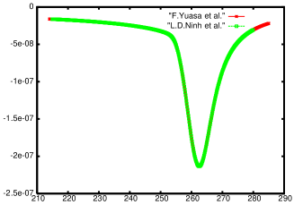
Figure 2: Integration result of the real part with complex masses as a function of $\sqrt{s_{2}}$. Our results agree to the 5- or 6-digit accuracy of Ninh’s.

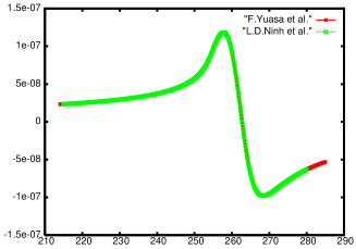
Figure 3: Integration result of the imaginary part with complex masses as a function of $\sqrt{s_{2}}$. Our results agree to the 4-, 5- or 6-digit accuracy of Ninh’s.

3.2 $e^{+}e^{-}\rightarrow ZZ\rightarrow e^{+}e^{-}Z$

The second example is the one-loop pentagon diagram in Fig. 4.

Figure 4: Diagram of $e^{+}e^{-}\rightarrow ZZ\rightarrow e^{+}e^{-}Z$

The loop integral is

$$I=\int_{0}^{1}dx_{1}dx_{2}dx_{3}dx_{4}dx_{5}\delta(1-\sum_{i=1}^{5}x_{i})\frac{1}{D^{3}}.$$ (1)

Here, $D({\bf x})$ is given as

$$D({\bf x}) = \sum_{i=1}^{5}m_{i}^{2}$$ (2)

$$- x_{1}x_{2}s_{1}-x_{2}x_{3}s_{2}-x_{3}x_{4}s_{3}-x_{4}x_{5}s_{4}$$

$$- x_{5}x_{1}s_{5}-x_{1}x_{3}s_{12}-x_{2}x_{4}s_{23}-x_{3}x_{5}s_{34}$$

$$- x_{4}x_{1}s_{45}-x_{5}x_{2}s_{51},$$

where $m_{1}=m_{3}=m_{4}=0.5\times 10^{-3}$ GeV and $m_{2}=m_{5}=91.00$ GeV. As an example, one numerical result is shown in Table 1 with a set of parameters corresponding to one phase space point (Table 2).

Table 1: Numerical result of one-loop pentagon.

	Result	Error
real	$0.4118519\times 10^{-13}$	$0.410\times 10^{-17}$
imag.	$-0.2336871\times 10^{-12}$	$0.619\times 10^{-16}$

These agree to the results by T. Ueda et al. [10].

Table 2: A set of parameters corresponding to one phase space point

Parameter	value
$S_{12}$	100000.00000
$S_{15}$	-14146.0960752976
$S_{23}$	-30471.3126018059
$S_{34}$	32384.1496580698
$S_{45}$	37833.5682283554

The elapsed time for the computation is about 9.3 hours for the real part using AMD Opteron 2.2 GHz CPU.

3.3 Two-Loop Self-energy

The third example is the two-loop self-energy diagram in Fig. 5.

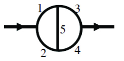
Figure 5: Diagram of the two-loop self-energy

The formulae of the loop integral is [11]

$$(16\pi^{2})^{2}I=\int_{0}^{1}dx_{1}dx_{2}dx_{3}dx_{4}dx_{5}\delta(1-\sum_{i=1}^{5}x_{i})\frac{1}{CD}.$$ (3)

Here, $D({\bf x})$ is given as

$$D({\bf x}) = -p^{2}(x_{5}(x_{1}+x_{3})(x_{2}+x_{4})$$ (4)

$$+ (x_{1}+x_{2})x_{3}x_{4}+(x_{3}+x_{4})x_{1}x_{2})$$

$$+ C{\tilde{M}^{2}},$$

$$C = (x_{1}+x_{2}+x_{3}+x_{4})x_{5}+(x_{1}+x_{2})(x_{3}+x_{4}),$$

$${\tilde{M}^{2}} = \sum_{i=1}^{5}x_{i}m_{i}^{2}.$$ (5)

We show the numerical results with two sets of the mass assignment shown in Table 3. The results with the first set are compared with ones by Kreimer [12] and by Kurihara et al. [13] in Fig. 6. The results with the second set are compared with ones by Kurihara et al. [13], by Bauberger et al. [14] and by Passarino et al. [15] in Fig. 7. In this computation, the elapsed time for the computation becomes longer around the singularities.

Table 3: Set of mass assignment in GeV

Set#	$m_{1}$	$m_{2}$	$m_{3}$	$m_{4}$	$m_{5}$
1	150.0	150.0	150.0	150.0	91.17
2	$\sqrt{1}.0$	$\sqrt{2}.0$	$\sqrt{4}.0$	$\sqrt{5}.0$	$\sqrt{3}.0$

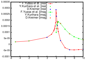
Figure 6: Numerical results of the loop integral with Set#1 mass assignment as a function of $p^{2}/150.0^{2}$. The results of [12, 13] are divided by the value of $p^{2}$.

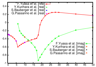
Figure 7: Numerical results of the loop integral with Set#2 mass assignment as a function of $p^{2}$. The sign of our numerical results is conformed to [13, 14, 15].

4 Parallel Computation

As we have described, the elapsed time for the computation becomes longer to get the sequence $\{I(\epsilon_{l})\}$ in a good accuracy when the singularity becomes steeper. To reduce the computation time, parallel computing technique is often used. We have developed the parallel code of Direct Computation Method. We used MPI library which is widely used in the parallel computing environment. We evaluated the speedup of the parallel code of DQ - and DE- Computation Method taking the integrals of two-loop vertex and one-loop box diagram as examples. The results of the speedup are shown in Table 4, Fig. 8 and Fig. 9. Both parallel codes show a good speedup behavior.

Table 4: Speedup of the parallel code of DQ-Direct Computation Method for the two-loop vertex diagram with singularities. We use PPC 970 and PC farm for the measurement. PPC 970 is IBM Blade CenterJS20 with PowerPC 970 2.2 GHz CPUs. PC farm consists of 16 Intel Xeon 3.06 GHz CPUs.

# of CPUs	PPC 970	PC farm
1	1.00	1.00
2	1.53	1.50
4	2.99	2.54
8	5.50	4.54
16		13.31

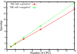
Figure 8: Speedup of the parallel code of DE-Direct Computation Method for the one-loop box integral with (DE-xd1-s-positive) and without (DE-xd1-s-negative) singularities. We use CRAY XD1 for the measurement.

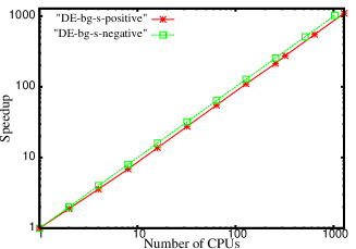
Figure 9: Speedup of the parallel code of DE-Direct Computation Method for the one-loop box integral with (DE-bg-s-positive) and without (DE-bg-s-negative) singularities. We use IBM BlueGene/L at KEK for the measurement.

5 Summary

In this paper, we presented several numerical results of the loop integrals by Direct Computation Method. This method is based on the combination of the numerical integration and an extrapolation technique. To reduce the computation time we developed the parallel code and the results of the speedup measurement are also shown.

References

• [1] E. de Doncker et al., Comput. Phys. Comm. 159 (2004) 145.
• [2] E. de Doncker et al., Nucl. Instr. Meth. A 534 (2004) 269.
• [3] E. de Doncker et al., LNCS 3514, (2005) 151.
• [4] F.Yuasa et al., PoS(ACAT)075
• [5] E. de Doncker et al., a talk in LoopFest V, June 19-21, 2006.
• [6] R. Piessens, et al., Springer Series in Computational Mathematics. Springer-Verlag, 1983.
• [7] H. Takahashi and M. Mori, Publication of RIMS, Kyoto University, vol.9 (1974) 721 and vol.41, no.4 (2005) 897.
• [8] P. Wynn, Math. Tables Automat. Computing 10 (1956) 91, and J. Numer. Anal. 3 (1966) 91.
• [9] F. Boudjema and L. D. Ninh, arXiv:0806.1498v2 and arXiv:0810.4078v1 [hep-ph].
• [10] T. Ueda et al., a talk in ACAT2008.
• [11] J. Fujimoto, et al., in New Computing Techniques in Physics Research II, World Scientific, 1992, p.625, Ed. by D.Perret-Gallix.
• [12] D. Kreimer, Phys. Lett. B273 (1991)277.
• [13] Y. Kurihara and T. Kaneko, Comput. Phys. Comm. 174 (2006) 530.
• [14] S. Bauberger et al., Nucl. Phys. B445 (1995) 25.
• [15] G. Passarino et al., Nucl. Phys. B629 (2002) 97.