Detection, Understanding, and Prevention
of Traceroute Measurement Artifacts

Abstract

Traceroute is widely used, from the diagnosis of network problems to the assemblage of internet maps. Unfortunately, there are a number of problems with traceroute methodology, which lead to the inference of erroneous routes. This paper studies particular structures arising in nearly all traceroute measurements. We characterize them as “loops”, “cycles”, and “diamonds”. We identify load balancing as a possible cause for the appearance of false loops, cycles, and diamonds, i.e., artifacts that do not represent the internet topology. We provide a new publicly-available traceroute, called Paris traceroute, which, by controlling the packet header contents, provides a truer picture of the actual routes that packets follow. We performed measurements, from the perspective of a single source tracing towards multiple destinations, and Paris traceroute allowed us to show that many of the particular structures we observe are indeed traceroute measurement artifacts.

1 Introduction

Jacobson’s traceroute [1] is one of the most widely used network measurement tools. It reports an IP address for each network-layer device along the path from a source to a destination host in an IP network. Network operators and researchers rely on traceroute to diagnose network problems and to infer properties of IP networks, such as the topology of the internet. This has led to an impressive amount of work in recent years [2, 3, 4, 5, 6, 7, 8], in which traceroute measurements play a central role.

Some authors have noticed that traceroute suffers from deficiencies that lead to the inference of inaccurate routes, in particular in the presence of load balancing routers [3, 4, 9]. However, no systematic study of these deficiencies has been undertaken. Therefore, people dealing with traceroute measurements currently have no choice but to interpret surprising features in traceroute measurements as either characteristics of the routing or of the network’s topology. This is supported by the common assumptions that these deficiencies have a very limited impact, and that, in any case, nothing can be done to avoid them.

The core contribution of this paper, which is a longer version of our earlier work [10], is to show that both of these assumptions are false. We show that the wide presence of load-balancing routers in the internet induces a variety of artifacts in traceroute measurements, and we provide a rigorous approach to both quantify and avoid many of them.

More precisely, we focus on three particular structures often encountered in traceroute measurements, which we categorize as “loops”, “cycles”, and “diamonds”. Using measurements from a single source tracing towards multiple destinations, we show that many instances of these structures are actually measurement artifacts resulting from load-balancing routers. We provide a new traceroute, called Paris traceroute,  which controls packet header contents to largely limit the effects of load balancing, and thus obtain a more precise picture of the actual routes. We show that many of the observed structures disappear when one uses Paris traceroute. Finally, we explain most other instances using additional information provided by Paris traceroute, and suggest possible causes for the remaining ones.

Throughout this paper, we use data obtained by tracing routes from one particular source to illustrate our results (see Sec. 3). From the outset, we insist on the fact that this data is not meant to be statistically representative of what can be observed on the internet in general: it serves as an illustration only, and the quantities reported may differ significantly from what would be observed from other sources. Obtaining a representative view of the average behavior of the traceroute tool would clearly be of interest, but is out of the scope of this paper: we focus here on the identification of traceroute artifacts, their rigorous interpretation, and their suppression using Paris traceroute.

This paper is structured as follows. Sec. 2 describes the classic traceroute tool, its deficiencies, and the new tool we built to circumvent these deficiencies, Paris traceroute. Sec. 3 describes our methodological framework. Sec. 4 categorizes the particular structures that we encounter and study in traceroute measurements. Sec. 5 and Sec. 6 study these structures, and provide our explanations for them. Sec. 7 discusses related work. Finally, Sec. 8 presents our conclusions and perspectives for future work.

2 Building a better traceroute

This section describes the tools used in this paper to study traceroute measurement artifacts. Sec. 2.1 describes the classic traceroute tool, and may be skipped by those familiar with it. Sec. 2.2 describes the deficiencies in classic traceroute in the face of load balancing. Sec. 2.3 then presents our new traceroute, Paris traceroute, which avoids some of these deficiencies, notably the ones induced by per-flow load balancing.

2.1 Traceroute

There are many varieties and derivatives of the traceroute tool. This section describes a generic probing scheme, based on Jacobson’s version [1]. Related tools, such as NANOG traceroute [11] and skitter [3], do very similar things. For a good detailed description of how traceroute works, see Stevens [12].

At a high level, three parameters define an invocation of the traceroute tool: the destination IP address, $d$, the probe packet protocol, $P$, and the number of probes per hop, $n$. The address $d$ may be any legal IP address. The protocol $P$ is one of either: UDP (by default), ICMP (also fairly common), or TCP (not used by the classic traceroute, but more and more used by other tools, such as tcptraceroute [13], because there is often less filtering of TCP packets).

Probing with traceroute is done hop by hop, moving away from the source towards the destination in a series of rounds. Each round is associated with a hop count, $h$. The hop count starts at one and is incremented after each round until the destination is reached, or until another stopping condition applies. A round of probing consists in sending $n$ probe packets with protocol $P$ towards destination $d$. By default $n$ is equal to three. The probe packets are sent with the value $h$ in the IP time-to-live (TTL) field.

The TTL of an IP packet is supposed to be examined by each router that the packet reaches. If the TTL is greater than one, then it is decremented and the packet is forwarded. If it is equal to one, the router drops the packet and sends an ICMP Time Exceeded message back to the source [14]. Routers are required to employ, as the source address of this ICMP message, the address of the IP interface that sends the ICMP packet [15, Sec. 4.3.2.4].  When routing is symmetric, this is typically the address of the interface that received the probe. The reception of a Time Exceeded message allows the traceroute tool to infer the presence of the source address at distance $h$ on the path to $d$.

The traceroute tool requires some means of matching return packets with the corresponding probe packets to know the correct sequence of IP addresses in the route to $d$. This is done by examining the payload of the Time Exceeded packet, which contains the beginning of the probe packet. More precisely, an ICMP Time Exceeded message contains the IP header of the probe packet, and the first eight octets that follow the IP header [17, p.5]. If the IP header contains no options, as is the case for traceroute probe packets, this amounts to the first 28 octets of the IP packet. The eight octets following the IP header comprise either the entirety of the UDP header, the entirety of the ICMP Echo header (the standard four octets of the ICMP header plus four octets for the Identifier and Sequence Number fields), or part of the TCP header, depending on $P$. If this portion of the probe packet contains a unique identifier, then traceroute can recognize the identifier in the Time Exceeded packet and match it to the corresponding probe. The default behavior of traceroute consists in setting the Source Port value of UDP probes to the running process identifier (PID) plus 32,768, and the initial Destination Port value to 33,435, and incrementing it with each probe sent. For ICMP Echo probes, the Sequence Number field is incremented with each probe sent [1].

For various reasons (such as routers dropping probes with a TTL of 1 without notifying the source, or routers on the reverse path dropping ICMP Time Exceeded messages), there might be no answer to a given probe. If, after a given time interval has elapsed, traceroute has not received an answer for a given probe, it stops waiting for it and outputs a star (‘*’) for the corresponding probe.

2.2 Traceroute and load balancing

Network administrators employ load balancing to enhance reliability and increase resource utilization. The main way to do so is through the intra-domain routing protocols OSPF [18] and IS-IS [19] that support equal cost multipath (ECMP). An operator of a multi-homed stub network can also use load balancing to select which of its internet service providers will receive which packets [20].

Routers can spread their traffic across multiple equal-cost paths using a per-packet, per-flow, or per-destination policy [21, 22]. In per-flow load balancing, packet header information ascribes each packet to a flow, and the router forwards all packets belonging to a given flow to the same path. This helps to avoid packet reordering within a flow. Per-packet load balancing makes no attempt to keep packets from the same flow together, and focuses purely on maintaining an even load on paths. This might be through round-robin assignment of packets to paths. The balance cannot be disturbed by the presence of out-sized flows. Finally, per-destination load balancing could be seen as a coarse form of per-flow load balancing, as packets are directed as a function of their destination IP address. But, as it disregards source information, there is no notion of a flow per se. As seen from the measurement point of view, per-destination load balancing is equivalent to classic routing, which is also per destination.

Concerning per-flow load balancing, a natural flow identifier is the five-tuple of fields from the IP header and either the TCP or UDP header: Source Address, Destination Address, Protocol, Source Port, and Destination Port. We performed some tests on some load-balancing routers from our traces to get an indication of which fields are used by routers to determine whether two packets belong to a same flow or not. We used TCP, UDP, ICMP, and IPSec probes. We sent probes from our laboratory to different destinations that cross the selected routers and varied header fields to observe which ones triggered load balancing. These tests showed that routers balance load using various combinations of the fields of the five-tuple, as well as three other fields: the IP Type of Service (TOS), and the ICMP Code and Checksum fields. We have not obtained answers from routers for ICMP probes of any type other than ICMP Echo, which means that we were unable to ascertain whether the ICMP Type field is also used for per-flow load balancing or not. Fig. 2 summarizes the IP, UDP, ICMP Echo, and TCP header fields that we observed are used by per-flow load balancers. We leave an exhaustive study of which parts of the header fields serve for load balancing, and in precisely which ways, to future work.

Finally, whether a router balances load per-packet, per-flow or per-destination depends on the router manufacturer, the OS version, and how the network operator configures it. For instance, Cisco and Juniper routers can be configured to do any of the three types of load balancing [21, 23, 22].

Traceroute, in consequence of its design, systematically sends probes via different paths in the presence of per-flow load balancing. This comes from its manipulation of the contents of the 28 first octets of the probes, in order to obtain a unique identifier. When sending UDP probes, it systematically varies the Destination Port field. When sending ICMP Echo probes, it varies the Sequence Number field. However, as explained above, varying these fields amounts to changing the flow identifier for each probe. The Destination Port field in the UDP header is used for flow identification, and, though the Sequence Number field is not directly used in this way, varying this field varies the Checksum field, which is a flow identifier.

Where there is load balancing, there is no longer a single route from a source to a destination. Classic traceroute is not only unable to uncover all routes from a source to a given destination, but it also proves unable to identify one single route from among many. It suffers from two systematic problems: it fails to discover routers and links, and it may uncover false links.

This is illustrated in Fig. 1. Here, $L$ is a load balancer at hop 6 from the traceroute source, $S$. On the left, we see the true router topology from hop 6 to hop 9. Circles represent routers, and each router interface is numbered. Black squares depict probe packets sent with TTLs 6 through 9. They are shown either above the topology, if $L$ directs them to router $A$, or below, if $L$ directs them to router $B$. On the right, we see the topology that would be inferred from the routers’ responses.

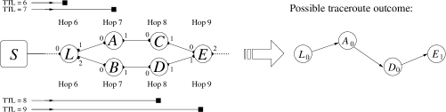
Figure 1: Missing routers and links, and false links.

Missing routers and links. Because routers $B$ and $C$ send no response, they are not discovered, and links such as $(L_{0},B_{0})$ and $(B_{0},D_{0})$ cannot be inferred. The probability of missing routers goes up with the number of routers at a given hop count: for instance, if there are four routers at a given hop, assuming that all probes have an equal probability of reporting each of the four routers, the probability of missing at least one of them when sending four probes is approximately equal to 0.78. Notice also that where there are missing routers, there are necessarily missing links as well. Finally, notice that the number of routers at a given hop count may be quite high: the newer Juniper routers, for instance, permit up to sixteen equal-cost paths.

False links. Independently of whether all routers (or links) are discovered or not, the traceroute tool lends itself to the inference of false links. In our example (Fig. 1), $L$ directs the probe with initial TTL 7 to $A$ and the one with initial TTL 8 to $B$, leading to the mistaken inference of a link between $A_{0}$ and $D_{0}$.

In our example, there is a probability $2/2^{4}=0.125$ that all probes to hops $7$ and $8$ follow an identical path. Thus, there is a probability of $0.875$ that addresses from routers on different paths will be revealed on subsequent hops, leading to false links impossible to differentiate from true ones in such measurements. Again, the presence of a high number of routers at a given hop count complicates the problem further by increasing the probability of inferring false links.

The problem of false links inferred from the appearance of multiple addresses on a same hop has been acknowledged in some cases, in particular by Huffaker et al. [3] and Spring et al. [4]. However, no systematic study of this phenomenon has been undertaken, and no real solution has been proposed.

2.3 A new traceroute

We now introduce Paris traceroute,  a new traceroute designed for networks with load-balancing routers. Its key innovation is to control the probe packet header fields in a manner that makes all probes towards a destination follow the same path in the presence of per-flow load balancing. It also makes it possible to distinguish between the presence of per-flow load balancing and per-packet load balancing, as we see below. Unfortunately, due to the random nature of per-packet load balancing, Paris traceroute cannot perfectly enumerate all paths in all situations. But it can do considerably better than the classic traceroute, and can flag those instances where there are doubts.

Maintaining certain header fields constant is difficult because traceroute needs to match response packets to their corresponding probe packets, and, as Fig. 2 shows, there is limited space in the probe packet headers in which to enable this matching (only the first 28 octets of the probe packet are encapsulated in the ICMP Time Exceeded response). Whithin this space, it is necessary to encode a packet identifier, and not all fields can be used for this purpose if the packets are to belong to a single flow. Also, to avoid ambiguity when there are multiple instances of the program running on the same machine, both traceroute and Paris traceroute encode a process identifier into the probe.

Some header fields, such as the IP Version, simply cannot be altered from their original purpose, as routers would tend to discard the packets as malformed. Other fields, such as the TTL, Source Address, and Destination Address, naturally cannot be altered. Nor would it be suitable to encode identifiers into the IP options, as packets with IP options are typically processed off the routers’ ‘fast path’ [24], meaning by different code, and thus with possibly different forwarding rules than the normal packets whose paths traceroute is supposed to trace. Finally, as we have mentioned, the IP TOS field and the first four octets of the transport layer header are off bounds as they are used for load balancing.

Paris traceroute uses the seventh and eight octets of the transport layer header as the packet identifier. In UDP probes, this is the Checksum field. However, simply setting the checksum value without regard to packet contents would create ill-formed probe packets liable to be discarded as corrupt. To obtain the desired checksum, Paris traceroute manipulates the UDP payload.

For ICMP Echo probes, Paris traceroute uses the Sequence Number field, as does classic traceroute. However, in classic traceroute this has the effect of varying the ICMP Checksum field, which is used for load balancing. Paris traceroute maintains a constant ICMP Checksum by changing the ICMP Identifier field to offset the change in the Sequence Number field.

Paris traceroute also sends TCP probes, unlike classic traceroute, but like Toren’s variant tcptraceroute [13]. To identify TCP probes, Paris traceroute uses the Sequence Number field (instead of the IP Identification field used by tcptraceroute). No other manipulations are necessary in order to maintain the first four octets of the header field constant.

To encode the process identifier, Paris traceroute uses the IP Identification field, whereas classic traceroute uses the Source Port for UDP probes, and the Identifier for ICMP Echo probes. Tcptraceroute does not encode a process identifier into its probe packets.

The simple fact of maintaining a constant five-tuple is not original to Paris traceroute, as tcptraceroute already does this for the TCP probes that it sends: in order to more easily traverse firewalls, tcptraceroute by default sets probes’ Destination Port field to 80, emulating web traffic. No prior work has, however, examined the effect of this choice with respect to load balancing.

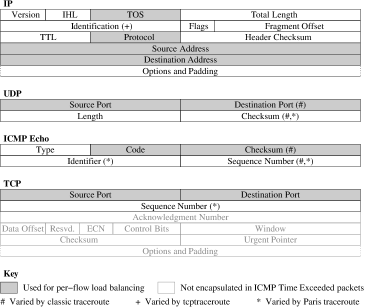
Figure 2: The roles played by packet header fields.

In addition to fixing the flow identifier problem, Paris traceroute provides additional information useful for recognizing certain other traceroute measurement artifacts. The probe TTL is the TTL that is found in the IP header of the probe packet encapsulated in the ICMP Time Exceeded response. This value corresponds to the probe’s TTL when the router received it and decided to discard it. Under normal traceroute behavior, this value is one. A value other than one reveals an error. The response TTL is the TTL of the Time Exceeded response itself. This value, available also through classic traceroute, helps in inferring the length of the return path. Finally, the IP ID is the Identification field from the IP header of the Time Exceeded response. This field is set by the router with the value of an internal 16-bit counter that is usually incremented for each packet sent. The IP ID can help identify the multiple interfaces of a single router, as described in the Rocketfuel work [4], or uncover different routers and hosts hidden behind a firewall or a NAT box, as described by Bellovin [25].

Finally, Paris traceroute may use different strategies for sending probes. PacketbyPacket behaves like the classic traceroute, i.e., sends a probe, waits for an answer or a timeout, sends the following probe, and so on. HopByHop sends all the probes for a given hop with a configurable delay between probes (the default value of this delay is 50 ms), waits for answers or timeouts, and then repeats the same procedure for the next hop. HopByHop is faster than PacketByPacket. Concurrent sends all the probes for all the hops with a configurable delay (default 50 ms) between probes. This algorithm is significantly faster than the previous two. To use Concurrent, however, one must know the number of hops needed to reach the destination. Scout sends one probe with a very high TTL to the destination. If the destination responds, then it estimates the number of hops needed to reach the destination and uses Concurrent. Otherwise, this strategy cannot be used. Scout is similar to the raceroute technique proposed by Moors [9].

Paris traceroute also allows the user to customize the minimum and maximum TTL values, in order to focus the measurement on a part of the path, and thus further speed up the measurements.

3 Measurement setup

This section explains how we conducted side-by-side measurements with classic traceroute and Paris traceroute, in order to study traceroute measurement artifacts.

Our measurement source was located at the LIP6 laboratory of the Université Pierre et Marie Curie, in Paris, France. The university has only one connection to the internet via the French academic backbone, Renater.

Our destination list consisted of 5,000 IPv4 addresses chosen at random, without duplicates, that answered to a ping probe at the time of the creation of the list. Following the lead of Xia et al. [26], we only considered pingable addresses so as to avoid the artificial inflation of traceroute measurement artifacts in our results that would come from tracing towards unused IP addresses.

For a period of $74$ days between June and August 2006, we performed 1,465 rounds of measurements by using classic traceroute and Paris traceroute to probe from our source to all destinations. This yielded the data set we use throughout this paper.

This data set serves as a case study, to show how one can identify, explain, and remove traceroute measurement artifacts with Paris traceroute. It is not intended to be representative of the statistics of traceroute measurement artifacts on the internet in general. We conducted several other measurements with similar setups and obtained results consistent with the ones we present below. Our results should therefore be considered as representative of what we observe from this source and under these measurement conditions, but statistics obtained from other vantage points, or towards other destination sets, may vary. Obtaining a representative view of what can be seen on average on the internet is clearly an interesting question, but it is out of the scope of this paper.

Each round of measurement was conducted in the following way. We launched 32 processes in parallel, that each probed $1/32^{nd}$ of the destination list. Each process selected, in turn, each destination $d$ from its portion of the list, and traced two routes to $d$, first using Paris traceroute, then using an instance of classic traceroute (NetBSD version 1.4a5). For both Paris traceroute and classic traceroute, we sent a single UDP probe for each hop, using the PacketByPacket strategy: waiting for a reply or a timeout from hop $h$ before sending the probe for hop $h+1$.  The chosen timeout was $2$ seconds. Paris traceroute kept the five-tuple of its probes constant during each instance of probing to a given destination, and selected Source and Destination Port values randomly from the range [10,000, 60,000]. Concerning classic traceroute, we kept the default behavior. The probing towards a given destination terminated when either the destination responded, or an ICMP message other than Time Exceeded was received. Moreover, Paris traceroute also stopped when TTL 36 was reached, or when eight consecutive stars were seen, whichever came first. Classic traceroute was set to stop if it reached a TTL of three greater than the last hop at which the previous run of Paris traceroute received an answer. Finally, we always set the minimal TTL to $2$ to skip the routers inside the university network.

One round of measurements to all destinations took approximately one hour and fifteen minutes, at the rate of approximately 27.3 seconds for both a Paris traceroute and a classic traceroute to a given destination.

For the $241$ million responses that contain valid IP Source Address values, we mapped the address to an AS number using Mao et al.’s technique [27]. Our data set covers 1,498 different ASes, which corresponds to six percent of the ASes in the internet today. Our data set covers all nine tier-1 ISP networks and 75 of the one hundred top-20 ASes of each region according to APNIC’s weekly routing table report.  Stars mostly appeared at the end of measured routes (when a destination does not answer, our measurement method induces many stars at the end of the corresponding measured route), with just $7.7$ million appearing in the midst of responses. We searched our measurements for invalid IP addresses, i.e., addresses that should not be given to any host on the public internet [28]. We found $11$ invalid IP addresses that account for $57$ thousand responses. None of these invalid addresses appear in the structures we study in the next section, and therefore they probably play little role in our observations.

Finally, we define a measured route to be the output of a given classic traceroute or Paris traceroute instance. Formally, a measured route is an $\ell$-tuple $\mathbf{r}=({r}_{0},\cdots,{r}_{\ell})$ where ${r}_{0}$ is the source address, and, for each $i$, $1\leqslant i\leqslant\ell,{r}_{i}$ stands either for the IP address received when probing with TTL $i$, or for a star if none was received. The integer $\ell$ is called the length of the measured route. We call any tuple of the form $(r_{i},r_{i+1},\dots,r_{i+k})$ a subroute of $\mathbf{r}$ of length $k$.

4 Structures under study

We focus our observations on three particular structures that appear in many measured routes: we call them loops, cycles, and diamonds. In this section we describe these structures, and present some basic statistics about their frequency of appearance in our traceroute data set. Sec. 4.1 discusses loops, Sec. 4.2 discusses cycles, and Sec. 4.3 discusses diamonds. In subsequent sections, we give possible causes and explanations for these structures, as well as methods for distinguishing between the different causes.

4.1 Loops

In some measured routes, the same IP address appears twice or more in a row: we call this a loop. In the normal course of routing, a router does not forward a packet back to the incoming interface. Hence, loops are most likely an artifact of the measurement itself. Formally, a loop is observed on IP address $r_{i}$ with destination $d$ if there is at least one measured route towards $d$ containing $\cdots,r_{i},r_{i+1},\cdots$ with $r_{i+1}=r_{i}$. The term ‘IP address’ implies that $r_{i}$ is not a star.

Load balancing can cause loops that appear sporadically when repeatedly tracing from a source to the same destination; this is shown in Fig. 3. These loops can occur in the presence of a load balanced route with at least two paths having a length difference equal to one.

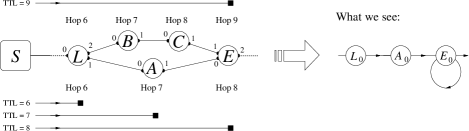
Figure 3: Loop caused by load balancing.

We call each observation of a measured route as described above a loop instance, and we define this loop’s signature as the pair $(r_{i},d)$. For instance, if we have four measured routes $(\ldots,a,a,b,\ldots,d_{1})$, $(\ldots,a,a,b,\ldots,d_{2})$, $(\ldots,a,a,b,$ $\ldots,d_{2})$ and $(\ldots,a,a,c,\ldots,d_{2})$, then we have four loop instances (one for each measured route), and two loops signatures ($(a,d_{1})$ and $(a,d_{2})$). Depending on the context, we will focus on statistics involving either loop signatures or loop instances. However, when the context is clear or when such distinction is irrelevant, we will simply use the term “loop”.

Moreover, we say that a measured route $\mathbf{r}$ contains a $n$-loop instance, with $n\geqslant 1$, on IP address $r$ when $r$ was observed on exactly $n+1$ consecutive positions on $\mathbf{r}$ ($n$ is the number of times $r$ is observed at two consecutive positions). We call $n$ the $length$ of the loop instance. The shortest loops are of length 1. We extend this definition to loop signatures: the length of a loop signature is the maximal length of all its instances.

Note that we use the term “loop” as meant commonly in graph theory. This is different from a forwarding loop, which typically involves several addresses. Forwarding loops are best described as cycles, which are discussed in Sec. 4.2.

Using the above definitions, enumerating loops is straightforward: we simply scan all the measured routes and look for instances of IP addresses that appear at least twice consecutively. To perform statistics, we maintain a list of all loop signatures encountered, and for each signature $(r,d)$ we keep a record of the relevant information: the number of instances, the maximal length, the number of times the IP address $r$ has been observed on measured routes towards $d$ (whether a loop has been observed or not), and so on.

Loops appear to be surprisingly common: overall, $7.51\%$ of the IP addresses detected in our experiment were in at least one loop instance, and more than $4.35\%$ of the measured routes contained a loop. Moreover, when probing repeatedly, say $N$ times to the same destination, the probability that at least one of the measured routes contained a loop increased with time; during our measurements, we were able to observe loops towards more than $24.6\%$ of the destinations. This is due to the high heterogeneity of loops: while some of them seem to be persistent and appeared on almost every measured route towards their destination, many others are occasional and appeared only once, or a couple of times. Measuring for a longer period of time therefore increased the probability of observing such occasional loops, within the duration of our experiments.  We also observed an intermediate behavior: systematic loops. We say that a loop $(r,d)$ is systematic if, whenever the IP address $r$ appeared in a measured route towards $d$, this occurrence was part of a loop. In other words, every time we saw $r$, we saw the loop.

The difference between systematic and persistent loops is that systematic loops don’t always show up on measured routes to a given destination, and may actually be exceptional. To examine this further, we defined two distinct characteristics. Consider a loop $(r,d)$ on address $r$ on a measured route towards a destination $d$:

1. Its appearance frequency is the probability that a measured route towards $d$ contained the loop.

2. Its conditional appearance frequency is the probability that a measured route towards $d$ that contained $r$ also contained the loop.

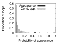
Figure 4: Dark bars: appearance frequency of the loops. Light bars: conditional appearance frequency of the loops.

Fig. 4 shows the distribution of these two characteristics over the loop signatures we observed. Notice that the proportion of persistent loops (appearance frequency close to $1$) seems to be very small, much smaller than the proportion of systematic loops (conditional appearance frequency close to $1$). However, since these loops were observed more often than the others, their proportion as instances was much more significant ($7.45\%$ of all instances).

Fig. 5 shows (left) the lengths of the $n$-loops we observed and their distributions among loop signatures (left) and loop instances (right). This chart is logarithmic, since large $n$-loops (i.e., with $n>1$) are very uncommon compared to $1$-loops. However, we observed several persistent large $n$-loops, which indicates that they shouldn’t be considered as marginal events.

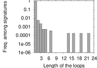
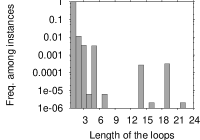
Figure 5: Distribution of the length of loop signatures (left) and instances (right).

Both length and appearance statistics confirm that several ‘flavors’ of loops exist. This points to the unlikelihood that all loops are generated by a unique mechanism, and suggests characterization of the loops into different categories, each of them resulting from a different cause.

4.2 Cycles

Formally, a measured route $\mathbf{r}$ is said to be cyclic on an IP address $r$, or $r$-cyclic, if it contains $r$ at least twice, at nonconsecutive locations, i.e., separated by at least one IP address $r^{\prime}$ distinct from $r$. The term ‘IP address’ implies that neither $r$ nor $r^{\prime}$ are stars. This distinction is to make sure we don’t misinterpret possible $n$-loops as cycles. For instance, a measured route $(\ldots,b,c,d,e,c,f,\ldots)$ is cyclic on $c$, but the measured route $(\ldots,b,c,*,*,c,f,\ldots)$ is not, since the sequence $c,*,*,c$ might well be a $3$-loop.

Load balancing can cause cycles, in the same way as loops; see Sec. 4.1 and Fig. 3. Cycles can occur when there is load balancing between routes having a length difference larger than one.

As for loops, we use the term cycle instance for any occurrence of a cycle on a measured route, and define a cycle signature as a pair $(r,d)$ of an IP address and a destination such that at least one of the measured routes towards $d$ is cyclic on $r$. Most of the cycles we observed occurred at more than one location on the measured routes, and sometimes they even overlap with each other, making it hard to define properties of a cycle as if it were a single, well-defined object. To be able to provide some statistics, we consider two properties. The length of a cycle signature $(r,d)$ is the shortest distance that separates two instances of $r$ in all measured routes towards $d$ that are $r$-cyclic. The span of a cycle signature $(r,d)$ is the greatest distance that separates two instances of $r$ in all measured routes towards $d$ that are $r$-cyclic. These properties capture respectively the minimal and maximal length of a round-trip from $r$ to $r$ observed on a measured route towards destination $d$. For instance, if we have three measured routes $(\ldots,r,a,b,r,\ldots,d_{1})$, $(\ldots,r,a,b,r,\ldots,d_{2})$ and $(\ldots,r,c,d,e,r,\ldots,d_{2})$, then the cycle signature $(r,d_{1})$ has both length and span equal to $3$, whereas the cycle signature $(r,d_{2})$ has a length of $3$ and a span of $4$.

An interesting species of cycles is the periodic cycles, which are encountered in measured routes like $(\ldots,a,b,c,b,c,\ldots)$. A measured route is $k$-periodically cyclic on IP addresses $r_{1},r_{2},\cdots,r_{k}$ when this sequence of IP addresses appear at least twice, consecutively, and in the same order, on the measured route. Formally, a periodic cycle signature is a pair $((r_{1},\cdots,r_{k}),d)$ such that at least one measured route towards $d$ is $k$-periodically cyclic on $r_{1},\cdots,r_{k}$.

As for loops, enumerating cycles consists in scanning every measured route, detecting the cycle instances, and aggregating information about every cycle signature encountered.

Cycles are less common than loops in our data set: they appeared on only $0.60\%$ of the measured routes. On the other hand, they appeared on a broad range of addresses: we observed cyclic measured routes towards $17.5\%$ of the destinations, and $4.73\%$ of the IP addresses discovered during our experiment appear in at least one cycle signature.

Fig. 6 presents appearance statistics similar to the ones already described for loops, using a similar terminology. To avoid redundancies, we invite the reader to consult Sec. 4.1 for definitions.

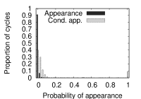
Figure 6: Dark bars: appearance frequency of cycles. Light bars: conditional appearance frequency of the cycles.

Persistent cycles appear to be very rare; they are actually invisible on Fig. 6. We did detect $2$ persistent cycles over the 5,674 cycle signatures we observed, and they account for $3.93\%$ of the cycle instances. Systematic cycles were more common (see the peak in Fig. 6 for a conditional appearance frequency of $1$), and represented $8.95\%$ of the cycle instances. They still have a very low appearance frequency, meaning that in spite of their systematic behavior, their occurrence remained infrequent in our measurements. Overall, it seems that cycles, unlike loops, are mostly occasional events. This makes them more difficult to track.

Fig. 7 shows the distribution of the length and span of the cycles we observed (as for loops, we both use the signature- and instance-based statistics). These statistics illustrate the variety of cycles that can be observed.

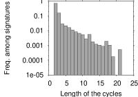
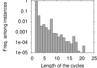
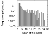
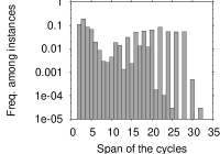
Figure 7: Distribution of the length (top) and span (bottom) of the cycles signatures (left) and instances (right).

From the distribution of the length of cycles, it is clear that cycles of length $2$ were predominant, especially for cycle instances. However, the cycles having a span of $2$ were not as common, and they were even outnumbered by cycles of span $3$ in terms of instances, which indicates that not all cycles of length $2$ also have a span equal to $2$. This is related to the observation that, for higher span values, cycles with an even span are much more likely to occur than those with odd span. These observations can be explained in terms of the periodic cycles we introduced earlier: a periodic cycle of period $2$ will have a length equal to $2$, and may have any even span between $2$ and the maximum number of hops allowed in our measurements.

This, plus the fact that cycles of extreme length also occurred regularly (according to the length distribution), also suggests the existence of a wide variety of phenomena as possible causes for cycles.

4.3 Diamonds

Loops and cycles are structures observed on single measured routes. Other types of structures in traceroute measurements appear only when multiple measured routes are considered together (e.g., when constructing maps of the network). A typical feature that we observe in this way is what we call a diamond.

Given a set $S$ of measured routes, a diamond is a pair $(h,t)$ of IP addresses for which the number $k$ of distinct IP addresses ${r}_{i}$ such that there exists a measured route in $S$ of the form $\ldots,h,{r}_{i},t,\ldots$ is at least $2$. The term ‘IP address’ implies that neither $h$, $t$, nor any of the $r_{i}$ are stars. We call $h$ the head of the diamond, and $t$ its tail. The core of the diamond is the set of addresses $\{{r}_{1},\ldots,{r}_{k}$}, and the diamond’s size is $k$.

Load balancing may induce many diamonds. Fig. 8 presents a typical such case.

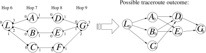
Figure 8: An example of several diamonds caused by load balancing. For clarity, we omit the probe packets.

Which diamonds we see depends upon which set $S$ of measured routes is considered. We will see in Sec. 5.3 that the distinctions between different types of diamonds afford interesting observations concerning load balancing.

A diamond $(h,t)$ that emerges from only the measured routes towards a single destination $d$ is called a $d$-diamond. If there exists at least one destination $d$ for which $(h,t)$ is a $d$-diamond, then we call $(h,t)$ a one-destination diamond. We define the size of a one-destination diamond $(h,t)$ to be the maximum of the sizes of all $d$-diamonds $(h,t)$.

A diamond $(h,t)$ that emerges from the entirety of measured routes in our data set is called a global diamond. All one-destination diamonds are also global diamonds.

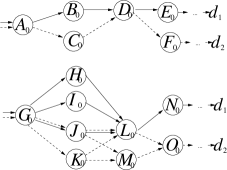
Figure 9: Examples of global diamonds, $d$-diamonds, and one-destination diamonds.

Fig. 9 presents examples of $d$-diamonds, one-destination diamonds, and global diamonds. We see measured routes towards two distinct destinations $d_{1}$ and $d_{2}$. $A_{0},\ldots,O_{0}$ are addresses observed on these measured routes, and a solid (respectively, dashed) arrow between two addresses indicates that they are linked in a measured route towards $d_{1}$ (respectively, $d_{2}$). $(G_{0},L_{0})$ is a $d_{1}$-diamond of size $3$, and a $d_{2}$-diamond of size $2$. Hence $(G_{0},L_{0})$ is also a one-destination diamond, and its size is $3$, which is the size of the largest $d$-diamond $(G_{0},L_{0})$. $(G_{0},M_{0})$, $(J_{0},O_{0})$ and $(K_{0},O_{0})$ are $d_{2}$-diamonds of size $2$ and also one-destination diamonds of size $2$. Note that $(A_{0},D_{0})$ is not a $d$-diamond for any $d$, and therefore not a one-destination diamond. $(A_{0},D_{0})$, $(G_{0},L_{0})$, $(G_{0},M_{0}$), $(J_{0},O_{0})$ and $(K_{0},O_{0})$ are global diamonds.

Diamonds are detected in the following manner: we scan every measured route, and maintain, for each possible triple $(h,t,d)$ of two IP addresses and a destination, the set $A_{d}(h,t)$ of all IP addresses seen between $h$ and $t$ on measured routes towards $d$. We then compute the set $A_{all}(h,t)$ of IP addresses seen between $h$ and $t$ on all measured routes by merging all the $A_{d}(h,t)$. For any destination $d$, the $d$-diamonds are then the pairs $(h,t)$ such that $|A_{d}(h,t)|\geqslant 2$. One-destination diamonds are the pairs $(h,t)$ such that there exists a $d$ such that $|A_{d}(h,t)|\geqslant 2$, and global diamonds are the pairs $(h,t)$ such that $|A_{all}(h,t)|\geqslant 2$.

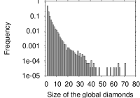
Figure 10: Distribution of the size of the global diamonds.

Overall, we observed 28,231 global diamonds in our traceroute data set. Fig. 10 presents their size distribution. They involved a very large fraction of the observed IP addresses: overall $44.6\%$ of the addresses were involved in global diamonds. Moreover, global diamonds were not separate entities but were highly interlocked with each other: $16.4\%$ of all addresses were in the head of one or more global diamonds, $30.7\%$ in the core, and $27.1\%$ in the tail. The sum of these proportions is much larger than $44.6\%$, which indicates that a large number of addresses belonged to several global diamonds.

One-destination diamonds and $d$-diamonds were also quite frequent in our measurements: there were 95,936 $d$-diamonds, and 24,326 one-destination diamonds. Among all destinations $d$, $90.2\%$ led to the observation of at least one $d$-diamond. The average number of distinct $d$-diamonds observed with these destinations was $21.3$.

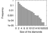
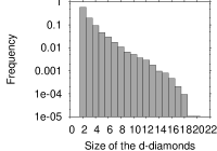
Figure 11: Distribution of the size of one-destination diamonds (left) and $d$-diamonds (right).

Fig. 11 presents the distribution of the size of $d$-diamonds and one-destination diamonds. We observe that there were far fewer large $d$-diamonds than global diamonds. This, together with the fact that there are more global diamonds than one-destination diamonds, indicates that measured routes towards different destinations combined with each other, creating global diamonds where there were no one-destination diamonds (as illustrated in Fig. 9), and increasing the size of existing one-destination diamonds to form large global diamonds.

5 Measurement artifacts due to load balancing

We now turn to the study of the differences observed when probing with Paris traceroute rather than with traceroute, for each of the three types of structures we study.

5.1 Loops

We compare the measurements obtained with classic traceroute and the ones obtained with Paris traceroute, the latter avoiding per-flow load balancing. Of the loop signatures, $89.8\%$ disappear; however, new loop signatures also appear, which represent approximately $2.73\%$ of the initial total. For loop instances, the statistics are $79.9\%$ and $0.21\%$. This shows that load balancing is likely the primary cause of loops in our observations. The fact that some loops are observed in our data set with Paris traceroute but not with classic traceroute most likely comes from the fact that some loops are rarely observed, as explained in Sec. 4.1. It is therefore natural that such loops might only be observed with one measurement tool and not the other.  These observations also hold for cycles and diamonds.

We investigate this matter further by looking at the characteristics of the loops removed by Paris traceroute. Fig. 12 shows the conditional appearance frequencies (see Sec. 4.1) of loops found in the traceroute and Paris traceroute data sets. One can see that almost all loops that were neither systematic nor truly rare, i.e., loops appearing sporadically, but somewhat regularly – which is the kind of behavior one would expect from loops caused by load balancing – are removed. At the same time, all persistent loops that appeared with traceroute were also present when using Paris traceroute, which was expected, since persistent loops are unlikely to be caused by load balancing. This will be discussed further in Sec. 6.

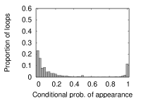
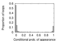
Figure 12: Conditional appearance frequencies of loops observed in our data set with classic traceroute (left) and Paris traceroute (right).

We also observe that $89.3\%$ of the non-persistent systematic loops disappear. We have seen how a load-balanced route with a pair of path lengths that differ by 1 can lead to the observation of a loop. We now hypothesize a router implementation of per-flow load balancing that would cause such a loop to be both systematic and non-persistent. We use Fig. 3 as an illustration. If the router $L$ were to forward probe packets in a round-robin fashion, alternatively to $B$ and to $A$, then our experiments would reveal only two measured routes out of the many that are possible: one with the subroute $(L_{0},B_{0},E_{0},E_{0})$ and one with $(L_{0},A_{0},C_{0},F_{0})$, where $F_{0}$ is the next hop beyond $E_{0}$. The first subroute contains a loop that is systematic, because it appears whenever $E_{0}$ appears, and that is non-persistent, because it only appears on a portion (in this case, 50%) of the routes to the destination.

What would account for such round-robin forwarding at a per-flow load balancer? Recall that per-flow load balancing assigns packets to outgoing interfaces as a function of the 5-tuple, and that classic traceroute increments the Destination Port by 1 with each subsequent probe, leaving the rest of the 5-tuple unchanged. We obtain the hypothesized behavior if the function employed by the router cycles through each interface in turn with each increment in the Destination Port.

These observations confirm that load balancing, be it flow-based or packet-based, is an important source of loops. However, we will see in Sec. 6 that some loops, which represent a significant part of the total ($7.45\%$), are not due to load balancing. This is true in particular for persistent loops.

5.2 Cycles

As for loops, we compare the cycles observed with classic traceroute and those obtained with Paris traceroute. We observe that $79.5\%$ of cycle signatures disappear under Paris traceroute, and that new signatures, representing $11.0\%$ of the initial total, appear. For cycle instances, these numbers are $39.7\%$ and $1.32\%$. The diagnosis here still is that load balancing is an important cause, and most probably the prominent one, for cycles. The low number of cycles caused by load balancing can be attributed to the unlikelihood of load balancing across paths having a length difference of two or more.

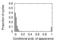
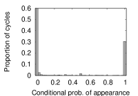
Figure 13: Conditional appearance frequencies of cycles observed in our data set with classic traceroute (left) and Paris traceroute (right).

As for loops, we also investigate the effect of Paris traceroute on the appearance frequency of cycles. Fig. 13 shows that cycles that are neither systematic nor very rare tend to disappear almost completely. This leads to the same conclusion: load balancing is an important cause of the appearance of cycles, and they are significantly reduced by the use of Paris traceroute.

5.3 Diamonds

We now compare the diamonds observed when using Paris traceroute to those observed with classic traceroute.

We observe far fewer global diamonds with Paris traceroute: $52.6\%$ of the diamonds observed with classic traceroute disappear; conversely, new global diamonds, representing $3.26\%$ of the total observed with traceroute, appear. Fig. 14 presents the distribution of the size of global diamonds observed with Paris traceroute.

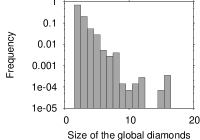
Figure 14: Distribution of the size of the global diamonds seen with classic traceroute (left) and Paris traceroute (right).

We observe that, not only are there far fewer global diamonds when using Paris traceroute, but their sizes are also greatly reduced. Moreover, they are less intertwined: $11.3\%$ of the IP addresses belong to at least one global diamond’s head, $24.8\%$ to a core, and $21\%$ to a tail. The sum of these proportions is 57.1, with overall $39.5\%$ of the addresses belonging to a global diamond (compared to $16.4\%$ of addresses in a global diamond’s head, $30.7\%$ to a core, $27.1\%$ to a tail, the sum of these proportions being $74.2$, with $44.6\%$ of all addresses belonging to a global diamond, for classic traceroute).

The number, size and complexity of $d$-diamonds and one-destination diamonds are also greatly reduced: $57.1\%$ of the $d$-diamonds and $56.9\%$ of the one-destination diamonds disappear; conversely, $2.18\%$ and $3.26\%$ of the total of $d$-diamonds and one-destination diamonds observed with traceroute appear. In addition, among all destinations $d$, $89.6\%$ lead to the observation of $d$-diamonds (compared to $90.2\%$ for classic traceroute), and each such destination leads on average to the observation of $9.7$ $d$-diamonds (compared to $21.3$ for classic traceroute). Fig. 15 presents the distribution of the size of $d$-diamonds observed with Paris traceroute.

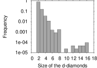
Figure 15: Distribution of the size of the $d$-diamonds seen with classic traceroute (left) and Paris traceroute (right).

This comparison gives an indication of the impact of per-flow load balancing on our observations. Diamonds that disappear when switching from classic traceroute to Paris traceroute are most probably induced by false links due to per-flow load balancing. $52.6\%$ of the global diamonds observed with traceroute disappear with Paris traceroute in our data set. This shows that diamonds are quite often (approximately half of the time) measurement artifacts induced by per-flow load balancing.

Studying diamonds also makes it possible to observe per-destination load balancing, by studying the differences between global diamonds and one-destination diamonds. To understand this, we must first notice that all diamonds indicate a priori the existence of alternative paths between our source and some router beyond the diamond. This can be seen as follows: if a given diamond is not a measurement artifact and does reflect the topology of the network, then it represents alternative paths between its head and its tail. False diamonds, caused by load balancing, also indicate the existence of alternative paths, but not necessarily between their head and tail. Consider the example of Fig. 8. In this case, the existence of three alternative paths between $L$ and $G$ induces the appearance of diamonds. Though there is only one path from $L$ to $D$, the diamond $(L_{0},D_{0})$ indicates the existence of alternative paths between some point, at its head or before it (in this case $L$), and some other point, at its tail or after it (in this case $G$).

Therefore, global diamonds that are not one-destination diamonds, and similarly global diamonds that are larger than corresponding one-destination diamonds, indicate the existence of alternative paths that can be explored only by probing towards different destinations; this corresponds to per-destination load balancing. In our case, the differences between global diamonds and one-destination diamonds are similar for traceroute and Paris traceroute: in both cases, global diamonds are larger than one-destination diamonds (this size difference is much more pronounced for traceroute than for Paris traceroute), and global diamonds that are not one-destination diamonds appear: there are 3,905 such global diamonds for traceroute, and 3,038 for Paris traceroute. We can therefore observe a significant quantity of per-destination load balancing in our data set.

Finally, notice that per-destination load balancing does not in itself induce false links, and therefore does not induce false diamonds: these are caused by the fact that probes for a same measured route follow different paths. A load balancer that directs packets depending on their destination, however, will direct all probes of a given measured route on the same path, because they all have the same destination.

Our observations showed different things. First, comparing diamonds obtained with the classic traceroute and Paris traceroute shows that many diamonds seen with traceroute are measurement artifacts caused by per-flow load balancing, and disappear when using Paris traceroute. This again shows that per-flow load balancing may have a strong impact on one’s observations with traceroute. Second, comparing global diamonds with one-destination diamonds allowed us to evaluate the amount of per-destination load balancing in our observations. Although this latter does not cause measurement artifacts in measured routes, being able to detect it leads to interesting observations.

Our studies open the way to more detailed analysis of both types of load balancing. We note however that, for this type of studies, other measurement strategies will probably need to be employed. Indeed, as we already mentioned, we observed in our data set that a small number of diamonds appear with Paris traceroute but not with classic traceroute. As explained in Sec. 4.1, this comes from the fact that some diamonds are observed very seldom, and might therefore be observed only with one tool and not the other. Some of these diamonds therefore could potentially be observed with Paris traceroute. A detailed study of load balancing should address this question.

Concerning diamonds seen with Paris traceroute, we observe that Paris traceroute is still subject to per-packet load balancing. These diamonds may therefore either reflect the real topology, or be false diamonds caused by per-packet load balancing or routing changes during the traceroute. Designing tools and measurement strategies allowing the statistical discovery of measurement artifacts caused by per-packet load balancing is an interesting and challenging direction of work; see Sec. 8.

6 Other causes of artifacts

In the previous section we have seen that most loops, most cycles, and approximately half of the diamonds observed in traceroute measurements disappear when using Paris traceroute. We will now study the ones that persist. We will see that Paris traceroute provides information that allows us to understand the causes of some of the remaining structures, and in some cases shows that they also are measurement artifacts.

The statistics we provide in this section are in regards to the set of structures yet unexplained by load balancing: unless stated otherwise, the percentages and ratios are to be taken as percentages and ratios among these remaining structures.

6.1 Zero-TTL forwarding

One explanation for loops comes from the traceroute manual, that mentions a bug in the standard router software of some BSD versions: these routers decrement the TTL of packets when it is equal to one, and forward the packet with TTL zero (whereas a normal router would drop the packet and generate an ICMP Time Exceeded message). Fig. 16 shows the consequence of the presence of such a router on a route trace.

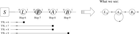
Figure 16: Loop caused by a misconfigured router (F) that forwards packets having TTL $0$.

We may validate the hypothesis of a misconfigured router with a simple experiment. Recall that Paris traceroute gives us the probe TTL: for any loop caused by zero-TTL forwarding, the probe TTL of the first response from the router involved in the loop would be zero. Fig. 17 shows how Paris traceroute would flag the loop in Fig. 16 with a “!T0”, indicating that the probe TTL returned for hop 7 was zero.

6  10.10.146.134  452.135 ms
7  10.10.127.197  452.246 ms !T0
8  10.10.127.197  450.898 ms
9  10.10.127.37   451.499 ms

Figure 17: Paris traceroute output for the example in Fig. 16.

We ran this validation test on all loops detected in our experiments. Of the persistent loop signatures we observed, $68.6\%$ were caused by zero-TTL forwarding. These represent $17.1\%$ of all the loop signatures that remained with Paris traceroute. Since persistent loops represent a significant part ($63.4\%$) of the loop instances observed with Paris traceroute, the number of loop instances that remain yet unexplained was reduced by $51.1\%$.

6.2 Routing Cycles

For cycles, the first explanation that comes to mind is that the packets do follow a cyclic route (often called a forwarding loop, but for clarity we will avoid this term here), and thus that the cycle is not an artifact of the measurement. The often long span of periodic cycles, their periodic behavior, and the fact that the observation of such cycles is typically associated with a measured route that does not reach the destination, argue for this.

We hypothesize that IP packets that do follow a cyclic route most likely do so because of a transient instability during routing convergence.  One observation that tends to validate this hypothesis is that almost all periodic cycles are transient, i.e., packets follow a normal route for some period before and after we observe the cycle. Note that this transient period may last longer than for just one route measurement: some periodic cycles were observed during a time span of as long as a week.

Moreover, we used Spring et al.’s [29] technique to verify that the identical IP addresses which form periodic cycles really come from the same router. This method is based on the fact that a large proportion of routers ($52\%$ in our data set) use an internal counter to assign ID fields to the packets they create, and increment it by $1$ every time a packet is sent (among the $48\%$ of remaining routers in our data set, more than $99\%$ of them use a constant ID value set to $0$). Packets sent within a short time period by a router using an internal counter have ID values that are close in regards to the $2^{16}=\text{65,536}$ possible values of this field. Since routers generate far fewer packets than they forward, this method can be applied on time windows as large as the duration of a full measured route (typically less than 30 s). While the observation of two packets having close ID fields is not a proof, the accumulation of such observations over time becomes strong evidence. We applied this method – when it was applicable – to our periodic cycles, since Paris traceroute provides the ID field of the response packet. We found a $100\%$ positive response, which shows that the periodic cycles we observe do in fact correspond to the actual routing. Routing cycles therefore represent $60.2\%$ of the cycle signatures, and $91.6\%$ of the cycle instances.

Finally, $43\%$ of the measured routes with periodic cycles actually reached the destination. According to a previous study of packet-level measurements in a large ISP backbone [30], most routing cycles last for less than $10$ seconds. This time is less than the average time of $30$ seconds needed to measure a route, so it seems reasonable to assume that packets may be caught in a cycle for some time, and then reach the destination. However, the study also found examples of routing cycles that persisted for $10$–$60$ seconds, which may be the explanation for cycles that do not end during our measurements.

6.3 Interrupted routes

Another explanation for loops, which also applies to cycles, comes from ICMP ‘unreachable’ responses. Some routers, when realizing that a packet cannot be delivered to its destination for some reason, may issue a special ICMP response, such as an ICMP Host Unreachable, Network Unreachable, or Source Quench (among others), and discard the probe. When receiving such responses, both classic traceroute and Paris traceroute consider that the route measurement has ended. Now, these routers may send these special responses even after having forwarded one or several probes. In this case, the router will appear twice on the measured route: once when it sends the normal ICMP Time Exceeded message, and once later when it sends the ICMP ‘unreachable’ packet.

We observe empirically that, most of the time in these cases, the router sends the unreachability message just after the Time Exceeded, leading to the observation of a loop. But sometimes it may also forward several probe packets between these two events, thus creating a cycle.

Tracking these events is easy, as Paris traceroute displays the type of ICMP received as answers, which allows us to filter out these messages. Interrupted routes represent $62.0\%$ of the loop signatures, and $27.0\%$ of the cycle signatures. In terms of instances, these numbers become respectively $19.7\%$ and $3.5\%$. The portion of instances is comparatively low since this type of measurement artifact is by essence occasional: most routers do not issue this type of message very often, and only a couple of loops and cycles that were caused by interrupted routes were observed persistently.

6.4 Fake IPs in return packets

Our last hypothesis for the presence of loops comes from the observation of the persistent $n$-loops. Some subnetworks are known to be impervious to traceroute measurements because they are behind NAT boxes and firewalls. In these networks the routers replace the Source Address field of the Time Exceeded packets on the way back to the probing machine, making them appear to come from their border gateway.

To validate this hypothesis, we tried to get some evidence that the consecutive replies from seemingly identical IP addresses actually came from different routers. The simplest way is to compare the TTL of the ICMP packets they send back: if the TTLs are different, then the responses likely came from different routers. This is even more obvious if these TTLs are always decreasing with distance (which indicates that the answering routers are in fact aligned on a route.)

We call fake loops the loops that are caused by this kind of Source Address replacement. We observed that $6.8\%$ of the loops signatures and $18.6\%$ of the loop instances came from such substituted IPs. The fake loops we detected were mostly persistent or systematic. One interesting result is that most of the persistent loops detected in our experiment that remained unexplained (i.e., not caused by zero-TTL forwarding) were determined to be fake loops. Another interesting result is that all persistent $n$-loops in our data set were fake.

The case of cycles caused by fake IPs is more puzzling, since the explanation based on protected subnetworks seems less plausible when observing non-consecutive responses with the same IP address. There are far fewer: only $1.6\%$ of the cycle signatures and $3.0\%$ of their instances seemed to be caused by it.

6.5 Summary

By considering per-flow load balancing, zero-TTL forwarding, routing cycles, interrupted routes, or fake IPs in return packet as causes for artifacts, we were able to explain roughly half of the diamonds, and more than $95\%$ of loops and cycles in our data set.

Table 1 presents the details of the proportions of loops (signatures and instances), cycles (signatures and instances) and diamonds (global diamonds and one-destination diamonds) caused in our data set by each phenomenon. In contrast to the other numbers presented in this section, the percentages in this table are with respect to all the structures observed in our data set: we do not restrict ourselves to the structures that remain with Paris traceroute. Since not all phenomena are possible causes of appearance for all structures, a dash ‘-’ indicates that a phenomenon does not apply to a structure.

Though our data are not representative, this illustrates how Paris traceroute helps understand and detect traceroute measurement artifacts. Regarding the unexplained structures, we suspect, after some preliminary studies, that most are artifacts caused by per-packet load balancing.

	Diamonds				Loops				Cycles
	global		$1$-dst		sign.		inst.		sign.		inst.
Per-flow load bal.	52.	6	56.	9	87.	1	79.	7	68.	5	38.	4
Zero-TTL fwd.	-		-		2.	21	10.	4	-		-
Routing cycles	-		-		-		-		19.	0	56.	4
Interrup. routes	-		-		8.	00	4.	00	8.	51	2.	16
Fake IP addresses	-		-		0.	88	3.	78	0.	50	1.	85
Unknown	47.	4	43.	1	1.	81	2.	15	3.	50	1.	17
Total	100.	00	100.	00	100.	00	100.	00	100.	00	100.	00

Table 1: Summary of identified measurement artifacts, showing the proportion of observed structures in our data that are attributed to each cause. All values are percentages.

7 Related work

We have earlier published a short version of this paper [10]. The present paper extends this preliminary work in several ways: the data set used here is much larger; we present here much more detailed analysis of loops and cycles; and the discussion on diamonds (Sec. 4.3 and 5.3) is almost completely new.

The principal variants on Jacobson’s traceroute [1] are Gavron’s NANOG traceroute [11], Eddy’s prtraceroute [31], and Toren’s tcptraceroute [13]. NANOG traceroute and prtraceroute both label IP addresses with the numbers of the ASes to which they belong. Tcptraceroute sends TCP probes (rather than the classic UDP or ICMP Echo probes) using Destination Port 80 to emulate web traffic and thus more easily traverse firewalls. As described in Sec. 2.3, this has the effect of maintaining a constant flow identifier. No prior work however has looked at the use of this feature to avoid traceroute measurement artifacts.

Although there is an extensive literature on internet maps, and much work that uses traceroute, there have been few studies of artifacts as seen from the perspective of traceroute. Moors [9] suggests that encoding traceroute probe packet identifiers in the Source Port field would allow the use of destination ports associated with classical services (e.g., HTTP or SMTP). This would cause all network elements, including load balancers, to handle these packets identically to the packets of normal network traffic. In doing so, he correctly identifies the problem that traceroute may not report routes that normal packets usually follow. However, the proposed solution still alters the five-tuple, and a tool built in this way would still suffer from load balancing and hence would present the same measurement artifacts as classic traceroute.

Paxson’s work on end-to-end routing behavior in the internet [32] uses traceroute to study routing dynamics, including “routing pathologies”. Although some of these pathologies do relate to the structures we discuss in this paper (for instance, “routing loops” are one cause of “cycles”, and “fluttering” is one cause of “diamonds”), his work focuses on the routing aspect of his observations and not on traceroute’s deficiencies. Teixeira et al. [33] examine inaccuracies introduced into ISP maps obtained by Rocketfuel [4]. Their paper quantifies differences between the true and the measured topologies, and identifies routing changes in the midst of individual traceroutes as being responsible for a portion of the false links in the measured topologies, but does not touch on load balancing.

Some topology inference systems based on traceroute acknowledge the problem that traceroute may report several interfaces at a same hop on a given path and thus may infer false links. They handle these problems in different ways. Huffaker et al. recognize the problem for skitter [3], but they do not report a solution. In practice, skitter sends three probes per hop and the routes reported by the arts++ tool for reading skitter data consist of the first address obtained for each hop. With Rocketfuel [4], Spring et al. attribute a lower confidence level to links inferred from hops that respond with multiple addresses. Still, they include all these links in the database from which they construct a network’s topology. Their hope is that a subsequent alias resolution step will eliminate at least some of the false links. However, this only works if load balancing takes place over multiple links between the same pair of routers.

8 Conclusion

In this paper, we identified and characterized three structures appearing frequently in traceroute measurements: loops, cycles, and diamonds. We explained how these structures, some of which are often attributed to routing dynamics or pathologies, may rather be measurement artifacts, induced notably by load balancing. We designed the Paris traceroute tool, a new traceroute that finds accurate routes under per-flow load balancing and proposed rigorous methods for checking the cause of each structure. By conducting side-by-side experiments with classic traceroute and Paris traceroute, we were able to show that most of these structures appearing in our traceroute traces are in fact measurement artifacts, and are avoided with Paris traceroute. Though our measurements are made from one source only and cannot be considered as statistically representative of what one can expect in the internet in general, this shows that per-flow load balancing can have a strong impact on one’s observations, and that the view obtained with Paris traceroute is more accurate.

This work may inspire future research in many directions. First, our experiments exposed other, rarer, structures than those described here, that also deserve attention: we observed cliques (sets of interfaces all linked to each other), dense regions, and IP addresses with a very high number of links. These structures are surprising, and may also be measurement artifacts.

Second, we believe that Paris traceroute can be further improved. We are working on an algorithm to automatically discover all paths between a source and a destination in the presence of per-flow load balancing. We are also developing techniques to uncover accurate routes in the presence of per-packet load balancing.

Finally, an important and interesting extension of this work is to perform measurements, both with classic traceroute and Paris traceroute, from several sources. This would make it possible to quantify the amount of traceroute measurement artifacts in the internet in general. We believe that new artifacts and features of interest will be observable when measurements originate from multiple sources. Moreover, one of the main conclusions of this work being that Paris traceroute provides a much truer view of the topology than existing tools, conducting measurements with Paris traceroute will yield data of higher quality for studying the topology of the internet. Studying the impact of using Paris traceroute on the observed topological properties is a very promising direction.

References

- [1] V. Jacobson, traceroute, the most recent version is available at: ftp://ftp.ee.lbl.gov/traceroute.tar.gz (February 1989).
- [2] R. Govindan, H. Tangmunarunkit, Heuristics for internet map discovery, in: Proc. IEEE Infocom, 2000.
- [3] B. Huffaker, D. Plummer, D. Moore, k claffy, Topology discovery by active probing, in: Proc. Symposium on Applications and the Internet, 2002.
- [4] N. Spring, R. Mahajan, D. Wetherall, Measuring ISP topologies with Rocketfuel, in: Proc. ACM SIGCOMM, 2002.
- [5] B. Cheswick, H. Burch, Internet Mapping Project, http://cm.bell-labs.com/who/ches/map/index.html (2000).
- [6] Y. Shavitt, E. Shir, DIMES: Let the internet measure itself, ACM SIGCOMM Computer Communication Review 35 (5) (2005) 71 – 74.
- [7] M. Faloutsos, P. Faloutsos, C. Faloutsos, On power-law relationships of the internet topology, in: Proc. ACM SIGCOMM, 1999.
- [8] D. Magoni, M. Hoerdt, Internet core topology mapping and analysis, ACM SIGCOMM Computer Communications 28 (5) (2005) 494–506.
- [9] T. Moors, Streamlining traceroute by estimating path lengths, in: Proc. IEEE Workshop on IP Operations and Management, 2004.
- [10] B. Augustin, X. Cuvellier, B. Orgogozo, F. Viger, T. Friedman, M. Latapy, C. Magnien, R. Teixeira, Avoiding traceroute anomalies with paris traceroute., in: Proc. ACM SIGCOMM Internet Measurement Conference, 2006.
- [11] E. Gavron, NANOG traceroute, the most recent version is available at: ftp://ftp.login.com/pub/software/traceroute/ (May 1995).
- [12] W. R. Stevens, TCP/IP Illustrated, Volume 1: The Protocols, Addison-Wesley, 1994, Ch. 8, Traceroute Program.
- [13] M. Toren, tcptraceroute, see http://michael.toren.net/code/tcptraceroute/ (April 2001).
- [14] J. Postel, Internet protocol, IETF RFC 791 (September 1981).
- [15] F. Baker, Requirements for IP Version 4 routers, IETF RFC 1812 (June 1995).
- [16] Z. M. Mao, J. Rexford, J. Wang, R. Katz, Towards an accurate as-level traceroute tool, in: Proc. ACM SIGCOMM, 2003.
- [17] J. Postel, Internet control message protocol, IETF RFC 791 (September 1981).
- [18] J. Moy, OSPF Version 2, IETF RFC 2328 (April 1998).
- [19] R. Callon, Use of OSI IS–IS for Routing in TCP/IP and Dual Environments, IETF RFC 1195 (December 1990).
- [20] B. Quoitin, S. Uhlig, C. Pelsser, L. Swinnen, O. Bonaventure, Interdomain traffic engineering with BGP, IEEE Communication Magazine 41 (5) (2003) 122–128.
- [21] Cisco, How does load balancing work?, see http://www.cisco.com/en/US/tech/tk365/technologies_tech_note09186a00800%94820.shtml.
- [22] Juniper, Configuring load-balance per-packet action, from the JUNOS 7.0 Policy Framework Configuration Guideline, see http://www.juniper.net/techpubs/software/junos/junos70/swconfig70-polic%y/html/policy-actions-config11.html.
- [23] Cisco, Cisco 7600 Series Routers Command References, from the Cisco Documentation.
- [24] R. Govindan, V. Paxson, Estimating router ICMP generation delays, in: Proc. of Passive and Active Measurement Workshop, 2002.
- [25] S. Bellovin, A technique for counting NATted hosts, in: Proc. ACM SIGCOMM Internet Measurement Workshop, 2002.
- [26] J. Xia, L. Gao, T. Fei, Flooding attacks by exploiting persistent forwarding loops, in: Proc. ACM SIGCOMM Internet Measurement Conference, 2005.
- [27] Z. M. Mao, D. Johnson, J. Rexford, J. Wang, R. H. Katz, Scalable and accurate identification of AS-level forwarding paths, in: Proc. IEEE Infocom, 2004.
- [28] IANA, Special-use IPv4 addresses, IETF RFC 3330 (September 2002).
- [29] N. Spring, M. Dontcheva, M. Rodrig, D. Wetherall, How to resolve IP aliases, UW CSE Technical Report (04-05-04).
- [30] U. Hengartner, S. B. Moon, R. Mortier, C. Diot, Detection and analysis of routing loops in packet traces, in: Proc. ACM SIGCOMM Internet Measurement Workshop, 2002.
- [31] R. Eddy, prtraceroute, the most recent version is part of the Internet Systems Consortium’s IRRToolSet, available from: http://www.isc.org/ (August 1994).
- [32] V. Paxson, End-to-end internet packet dynamics, IEEE/ACM Trans. Networking 7 (3) (1999) 277–292.
- [33] R. Teixeira, K. Marzullo, S. Savage, G. M. Voelker, In search of path diversity in ISP networks, in: Proc. ACM SIGCOMM Internet Measurement Conference, 2003.