Renormalization-group properties of transverse-momentum dependent parton distribution functions in the light-cone gauge with the Mandelstam-Leibbrandt prescription

Abstract

The renormalization-group properties of transverse-momentum dependent parton distribution functions in the light-cone gauge with the Mandelstam-Leibbrandt prescription for the gluon propagator are addressed. An expression for the transverse component of the gauge field at light-cone infinity, which plays a crucial role in the description of the final-/initial-state interactions in the light-cone axial gauge, is obtained. The leading-order anomalous dimension is calculated in this gauge and the relation to the results obtained in other gauges is worked out. It is shown that, using the Mandelstam-Leibbrandt prescription, the ensuing anomalous dimension does not receive contributions from extra rapidity divergences related to a cusped junction point of the Wilson lines.

I Introduction

Parton distribution functions (PDF)s contain nonperturbative information about the intrinsic structure of hadrons in terms of their constituents—quarks and gluons Col03 ; BR05 ; Col08 . In completely inclusive processes (e.g., deeply inelastic scattering (DIS), where the hard virtual photon with momentum $q^{2}=-Q^{2}$ probes a hadron $h$ with momentum $P$), integrated PDFs $f_{i}(x,Q^{2})$ ($i$ marking the sort of parton) depend on the longitudinal-momentum fraction $x$, which becomes equal to the Bjorken variable $x_{\rm B}$ in the limit $Q^{2}\to\infty$, $x_{\rm B}=Q^{2}/2(q\cdot P)=\hbox{const}$, and on the scale of the hard subprocess $Q^{2}$. In the Bjorken limit, these distributions (Feynman parton densities) are related to the (unpolarized) quark and antiquark structure functions

$$F_{1}(x_{\rm B},Q^{2})=\frac{1}{2x_{\rm B}}\ F_{2}\left(x_{\rm B},Q^{2}\right)=\frac{1}{2}\sum_{i}\ e_{i}^{2}\left[f_{i}(x_{\rm B},Q^{2})+{\bar{f}}_{i}(x_{\rm B},Q^{2})\right]$$ (1)

in the leading-twist approximation and in leading order of the coupling $\alpha_{s}$ (where $e_{i}$ is the electric charge of the quark of flavor $i$) AP77 . Equation (1) originates from the DIS factorization expression

$$F_{1}(x_{\rm B},Q^{2})=\sum_{i}\ \int_{x_{\rm B}}^{1}\!\frac{dz}{z}\ C_{1i}\left[\frac{x_{\rm B}}{z},\frac{Q^{2}}{\mu^{2}},\alpha_{s}(\mu)\right]\ \left[f_{i}(z,\mu^{2})+{\bar{f}}_{i}(z,\mu^{2})\right]\ ,$$ (2)

where the perturbative coefficient functions $C_{1i}$ are taken in leading order (LO): $C_{1i}^{\rm LO}=\frac{1}{2}e_{i}^{2}\ \delta(x/z-1)$. It can be considered as a triumph of perturbative QCD that the QCD evolution correctly describes the logarithmic dependence of the parton densities on the hard scale $Q^{2}$ and is, therefore, able to explain the experimentally observed violation of the Bjorken scaling. Moreover, the gauge-invariant operator definition of integrated PDFs

$$f_{i/h}(x,Q^{2})=\frac{1}{2}\int\frac{d\xi^{-}}{2\pi}\hbox{e}^{-ik^{+}\xi^{-}}{\langle h|}\bar{\psi}_{i}(\xi^{-}){\cal P}\exp\left[-ig\int_{0^{-}}^{\xi^{-}}\!\!dz^{\mu}A^{a}_{\mu}(z)t^{a}\right]\gamma^{+}\psi_{i}(0^{-}){|h\rangle}\Bigg{|}_{\xi^{+},\,\xi_{\perp}=0}$$ (3)

with $k^{+}=xP^{+}$ allows one to relate their moments to the matrix elements of the twist-two operators arising in the operator product expansion (OPE) on the light-cone CS82 . The renormalization properties of these PDFs are governed by the DGLAP equation AP77 ; DGLAP , establishing the logarithmic dependence on $Q^{2}$ mentioned above.

The study of semi-inclusive processes, such as semi-inclusive deeply inelastic scattering (SIDIS), or the Drell-Yan (DY) process—where one more final or initial hadron is detected and its transverse momentum is observed—requires the introduction of more complicated quantities, viz., unintegrated, i.e., transverse-momentum dependent (TMD) distribution or fragmentation functions:

$$\hbox{semi-inclusive}\ \ \to\ \ f_{i/h}(x,\mbox{\boldmath$k$}_{\perp},Q^{2})\ .$$ (4)

The most natural generalization of the operator definition (3), respecting gauge invariance and collinear factorization, reads CS81 ; CS82 ; Col03 ; JY02 ; BJY03 ; BMP03

$$f_{i/h}\left(x,\mbox{\boldmath$k_{\perp}$};\mu^{2}\right)=\frac{1}{2}\int\frac{d\xi^{-}d^{2}\mbox{\boldmath$\xi_{\perp}$}}{2\pi(2\pi)^{2}}{\rm e}^{-ik^{+}\xi^{-}+i\mbox{\footnotesize\boldmath$k_{\perp}$}\cdot\mbox{\footnotesize\boldmath$\xi_{\perp}$}}\left\langle h|\bar{\psi}_{i}(\xi^{-},\mbox{\boldmath$\xi_{\perp}$})[\xi^{-},\mbox{\boldmath$\xi_{\perp}$};\infty^{-},\mbox{\boldmath$\xi_{\perp}$}]^{\dagger}\right.$$

$$\left.\times[\infty^{-},\mbox{\boldmath$\xi_{\perp}$};\infty^{-},\mbox{\boldmath$\infty_{\perp}$}]^{\dagger}\gamma^{+}[\infty^{-},\mbox{\boldmath$\infty_{\perp}$};\infty^{-},\mbox{\boldmath$0_{\perp}$}][\infty^{-},\mbox{\boldmath$0_{\perp}$};0^{-},\mbox{\boldmath$0_{\perp}$}]\psi_{i}(0^{-},\mbox{\boldmath$0_{\perp}$})|h\right\rangle\ \,,$$ (5)

where gauge invariance is ensured by means of the path-ordered Wilson-line operator (gauge link) with the generic form

$${[y,x|\Gamma]}={\cal P}\exp\left[-ig\int_{x[\Gamma]}^{y}dz_{\mu}A_{a}^{\mu}(z)t_{a}\right]\ .$$ (6)

The transverse gauge links extending to light-cone infinity are also included in (5) and the dependence on $Q^{2}$ is taken into account via the renormalization-group (RG).

However, as it has been pointed out in CS81 , when one retains in the parton densities the intrinsic transverse momentum, extra undesirable divergences appear. These divergences are associated with the particular features of the light-cone gauge (or the use of purely lightlike Wilson lines) that must be removed by some consistent method (see, e.g., Col08 ; CRS07 ; Bacch08 ; CS07 ; CS08 ). For instance, they can be avoided by using non-lightlike gauge links in covariant gauges, or by employing an axial gauge, but going off-the-light-cone CS81 ; JMY04 . This involves the introduction of an extra rapidity parameter and entails an additional evolution equation CS81 , rendering the reduction to the integrated PDF questionable.

Another strategy, based on a subtraction formalism of these extra divergences in terms of a “soft” factor (defined as the vacuum average of particular Wilson lines and amounting to a generalized renormalization of TMD PDFs), was presented in Refs. CH00 ; Hau07 ; CM04 ; CS07 ; CS08 . The major finding in our previous investigations in CS07 ; CS08 was that, adopting the light-cone gauge, the leading gluon radiative corrections associated with the transverse gauge link were found to give rise to an extra term in the anomalous dimension of the TMD PDF that exhibits a $\ln p^{+}$ behavior—characteristic of a contour with a cusp. The new definition for the TMD PDF, proposed in these works, has two important advantages: (i) it reduces to the correct integrated case and (ii) it coincides with the result obtained in the Feynman gauge that is untainted by contour obstructions.

In (non-covariant) axial gauges the partonic interpretation of the distribution functions is preserved because the gauge links can be set to unity under the gauge condition. It is well-known that among the axial light-cone gauges there is one which has important advantages. Indeed, employing the light-cone gauge in association with the Mandelstam-Leibbrandt (ML) prescription Man83 ; Lei84 in the calculation of the quark self-energy and the quark-quark-gluon vertex LN83 ; BA96 , and also the DGLAP kernel in NLO BHKV98 , it was shown that no undesirable singularities appear—even at the intermediate steps of the calculation—in contrast to the principal-value (PV) prescription used in CFP80 . In the ML-gauge, the contributions of the real and the virtual diagrams are well-defined in the “end-point” region separately. [This is the region proportional to the delta-function of the longitudinal fraction of the hadron’s momentum $\sim\delta(1-x)$]. In the calculation of the evolution of the inclusive (integrated) PDF, this is not important—at least in LO—since all these singularities cancel in the final result. But the situation changes for the unintegrated TMD PDFs. In that case, the spacelike distance between the quark operators in the corresponding matrix elements acts like an ultraviolet (UV)-regulator, thus preventing the mutual cancelation of the extra (mixed) divergent terms between the virtual and the real gluon contributions. As a result, the rapidity divergences contributing to the UV-divergent part of the self-energy graph remain uncanceled. Exactly those terms of the splitting function, arising from the “end-point” region, give rise to extra (mixed) UV-singularities in the TMD function that can be eliminated by employing the ML-prescription—even extending the calculation to the NLO BHKV98 .

From the field-theoretical point of view, the ML-gauge has very attractive properties as well. Due to the position of the poles in the same quadrants as for the free gluon propagator (see Fig. 1), one can readily perform the Wick rotation to the Euclidean space. This is not possible for the $q^{-}$-independent prescriptions. Thus, in the ML-gauge, the standard power counting rules allow one to estimate the UV-divergences. Moreover, is has been shown that the ML-prescription arises naturally in a consistent quantization procedure BDLS84 ; BDS87 ; SF87 .

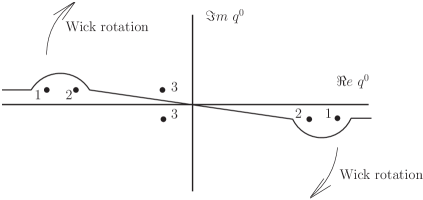
Figure 1: Integration contour and poles in the $(\hbox{\bf Re}\ q^{0},{\textbf{Im}{}}\ q^{0})$ plane: the poles of the gluon propagator using the ML-prescription (position 1) and those in a covariant gauge (position 2) belong to the same, i.e., second and fourth, quadrants. This is in contrast to the poles pertaining to the principal-value prescription (position 3). The Wick rotation can be performed without changing the position of the poles.

We have pointed out recently CS07 ; CS08 that the renormalization-group properties of TMD PDFs can be profitably analyzed in terms of their UV anomalous dimensions. The main reason is that anomalous dimensions are local quantities originating from the geometrical obstructions of the gauge contours: endpoints, cusps, or self-intersections. Within this context, gauge-invariant quantities have to fulfil anomalous-dimension sum rules that represent logarithmic, i.e., additive, versions of the Slavnov-Taylor identities CS08 . In our previous works all the calculations have been done in the light-cone axial gauge with additional $q^{-}$-independent pole prescriptions, notably, the advanced, retarded, and the principal-value one. It was shown that the extra contribution to the anomalous dimension of the TMD PDF, given by Eq. (5), can be identified (at least in the one-loop order) with the well-known cusp anomalous dimension KR87 . In the present investigation we apply this type of approach to a pole configuration of the gluon propagator controlled by the ML prescription. In what follows, we shall first analyze (Sec. II) the behavior of the transverse component of the (“classical”) gauge field at light-cone infinity—required for the derivation of the transverse gauge link that eliminates the residual gauge freedom (after fixing the gauge by $A^{+}=0$)—and derive an explicit expression for the gauge field in the ML-gauge. Then, we shall calculate the UV-divergent parts and the corresponding anomalous dimension of the TMD PDF (Sec. III). It is remarkable that the result obtained this way is free of undesirable terms related to contour obstructions and coincides with the double anomalous dimension of the fermion field. As we shall show later (Sec. IV), the crucial point in verifying the validity of the modified definition of TMD PDFs, Eq. (27) below, proposed in CS07 ; CS08 , is that the so-called mixed rapidity divergences are absent in the ML-gauge, while the contribution of the soft factor (which has been introduced in order to cancel these divergences in the case of $q^{-}$-independent prescriptions) reduces to unity in the one-loop order—see Sec. V. Our conclusions are presented in Sec. VI.

II Transverse gauge field at light-cone infinity in the ML-gauge

It was argued in Refs. JY02 ; BJY03 that in order to restore the contribution of the gluon exchanges between the struck quark and the spectator in the light-cone gauge, one has to take into account the accumulation of the corresponding phase in the transverse direction [Note that this phase is suppressed in covariant gauges]. It is precisely this phase that yields the additional transverse gauge link at light-cone infinity, introduced in Refs. JY02 ; BJY03 ; BMP03 , the reason being that this phase is accumulated very slowly. Below, we derive an expression for the gauge field in this situation by adopting the ML-prescription. This has not been considered before in the literature.

We commence our analysis by calculating the gauge field, the source of which is a “classical” current

$$j_{\mu}(y)=g\int\!dy^{\prime}_{\mu}\ \delta^{(4)}(y-y^{\prime})\,,\quad y^{\prime}_{\mu}=v_{\mu}\ \tau\ ,$$ (7)

corresponding to a charged point-like particle (e.g., a struck quark in a SIDIS process) and moving with the quasi-constant four-velocity $v_{\mu}$ along the straight line $v_{\mu}\tau$. Note that the velocity changes only at the origin, where the sudden collision with the hard photon takes place and the quark is derailed to its new “trajectory”. The gauge field related to such a current is given by

$$A^{\mu}(\xi)=\int\!d^{4}y\ {\cal D}^{\mu\nu}(\xi-y)j_{\nu}(y)\ \ ,$$ (8)

where $D^{\mu\nu}$ is the gluon Green’s function. We assume that the velocity of the struck quark is parallel to the “plus”- and the “minus”- light-cone vectors $n^{\pm}_{\mu}$ before and after the hard collision, respectively:

$$j_{\mu}(y) = g\left[n^{+}_{\mu}\int_{-\infty}^{0}\!d\tau\ \delta^{(4)}(y-n^{+}\tau)+n^{-}_{\mu}\int_{0}^{\infty}\!d\tau\ \delta^{(4)}(y-n^{+}\tau)\right]$$ (9)

$$= g\ \delta^{(2)}(\mbox{\boldmath$y$}_{\perp})\left[n^{+}_{\mu}\delta(y^{-})\int\!\frac{dq^{-}}{2\pi}\frac{\hbox{e}^{-iq^{-}y^{+}}}{q^{-}+i0}-n^{-}_{\mu}\delta(y^{+})\int\!\frac{dq^{+}}{2\pi}\frac{\hbox{e}^{-iq^{+}y^{-}}}{q^{+}-i0}\right]\ .$$

Using the results of Refs. CS07 ; CS08 , we write

$$A^{\mu}(\xi)=-g\ n_{\nu}^{+}\int\!\frac{d^{4}q}{2(2\pi)^{4}}\ {\hbox{e}^{-iq\cdot\xi}}\ \tilde{\cal D}^{\mu\nu}(q)\int\!dy^{+}dy^{-}d^{2}y_{\perp}{\hbox{e}^{iq\cdot y}}\delta(y^{-})\delta^{(2)}(\mbox{\boldmath$y$}_{\perp})\ ,$$ (10)

where the free gluon propagator in the light-cone gauge $A^{+}=0$ has the form

$${\cal D}^{\mu\nu}(z)=\int\!\frac{d^{4}q}{(2\pi)^{4}}\ {\hbox{e}^{-iq\cdot z}}\tilde{\cal D}^{\mu\nu}(q)=-\int\!\frac{d^{4}q}{(2\pi)^{4}}\ \frac{\hbox{e}^{-iq\cdot z}}{q^{2}+i0}\left(g^{\mu\nu}-\frac{q^{\mu}(n^{-})^{\nu}+q^{\nu}(n^{-})^{\mu}}{[q^{+}]}\right)$$ (11)

with the square bracket being used in order to remind that $[q^{+}]$ has yet to be defined. Here, and in what follows, we neglect the quark and gluon masses $m$ and $\lambda$, since we are mainly interested in the UV-singularities.

Performing the integration over the variable $y$, we get

$$A^{\mu}(\xi)=-g\ n_{\nu}^{+}\int\!\frac{d^{4}q}{2(2\pi)^{4}}\ {\hbox{e}^{-iq\cdot\xi}}\ \frac{\delta(q^{-})}{q^{2}+i0}\ \left(g^{\mu\nu}-\frac{q^{\mu}(n^{-})^{\nu}+q^{\nu}(n^{-})^{\mu}}{[q^{+}]}\right)\ .$$ (12)

Before continuing, let us first verify that the longitudinal (light-cone) components of the gauge field vanish and that there is no contradiction with the gauge condition. The “plus”-component reads

$$A^{+}=(A^{\mu}\cdot n^{-}_{\mu})\sim n^{-}_{\mu}\left((n^{+})^{\mu}-\frac{q^{\mu}+q^{-}(n^{-})^{\mu}}{[q^{+}]}\right)=1-\frac{q^{+}}{[q^{+}]}\ .$$ (13)

Notice that one has for both types of pole prescriptions: $q^{-}$-independent, as well as for $q^{-}$-dependent ones (like the ML-prescription), $q^{+}/[q^{+}]=1$ (see, e.g., Ref. CDL83 ), so that

$$A^{+}=0\ ,$$

a result in agreement with the light-cone gauge. One the other hand, for the “minus”-component, we start with

$$A^{-}=(A^{\mu}\cdot n^{+}_{\mu})\sim n^{+}_{\mu}\left((n^{+})^{\mu}-\frac{q^{\mu}+q^{-}(n^{-})^{\mu}}{[q^{+}]}\right)=0-\frac{2q^{-}}{[q^{+}]}\ ,$$ (14)

and carrying out the integration over $q^{-}$ in Eq. (12) with $\delta(q^{-})$, we find

$$A^{-}=0\ .$$

Now turn to the evaluation of the transverse components. Let us recall that employing $q^{-}$-independent prescriptions, the transverse component of the gauge field is

$$\mbox{\boldmath$A$}^{\perp}(\infty^{-};\mbox{\boldmath$\xi$}_{\perp})=\frac{g}{4\pi}C_{\infty}\ \mbox{\boldmath$\nabla$}^{\perp}\ln\ \Lambda|\mbox{\boldmath$\xi$}_{\perp}|\,,$$ (15)

where the numerical constant $C_{\infty}$ depends on the pole prescription according to (see BJY03 )

$$C_{\infty}=\left\{\begin{array}[]{ll}&\ \ 0\ ,\ {\rm Advanced}\\ &-1\ ,\ {\rm Retarded}\\ &-\frac{1}{2}\ ,\ {\rm Principal~{}Value~{}}\ .\end{array}\right.$$ (16)

Here $\Lambda$ is an IR-regulator that does not enter the final results.

The ML-prescription, being dependent on both variables $q^{+}$ and $q^{-}$, gives rise to a more complicated pole structure in the complex $q^{0}$ plane, viz.,

$$\frac{1}{[q^{+}]_{\rm ML}}=\left\{\begin{array}[]{ll}&\ \ \frac{1}{q^{+}+i0q^{-}}\\ &\ \ \frac{q^{-}}{q^{+}q^{-}+i0}\end{array}\right.\ .$$ (17)

The two possible forms of this prescription, displayed in Eq. (17), are, in fact, equivalent to each other. After performing the integral over $y$ in Eq. (10), one finds

$$\mbox{\boldmath$A$}^{\perp}(\xi)=-g\ \pi\int\!\frac{d^{4}q}{2(2\pi)^{4}}\ {\hbox{e}^{-iq\cdot\xi}}\ \frac{\delta(q^{-})}{q^{2}+i0}\ \left((n^{+})^{\perp}-\frac{q^{\perp}+q^{-}(n^{-})^{\perp}}{[q^{+}]_{\rm ML}}\right)\ .$$ (18)

Taking into account that the light-cone vectors $n^{\pm}$ have only longitudinal components and separating out the transverse integrations, we get

$$\mbox{\boldmath$A$}^{\perp}(\xi)=g\ \pi\int\!\frac{d^{2}q_{\perp}}{(2\pi)^{2}}\ \mbox{\boldmath$q$}^{\perp}\ \hbox{e}^{iq_{\perp}\xi_{\perp}}\int\!\frac{dq^{+}dq^{-}}{(2\pi)^{2}}\ \delta(q^{-})\ \frac{\hbox{e}^{-i(q^{+}\xi^{-}+q^{-}\xi^{+})}}{(q^{2}+i0)[q^{+}]_{\rm ML}}\ \ .$$ (19)

In order to compute the longitudinal part of this expression, we use for the denominator the $\alpha$-representation and employ for the delta-function the integral representation

$$\delta(q^{-})=\frac{1}{2\pi}\int_{-\infty}^{\infty}\!d\lambda\ \hbox{e}^{iq^{-}\lambda}\ .$$

This allows us to write

$$\int\!\frac{dq^{+}dq^{-}}{(2\pi)^{2}}\ \ \delta(q^{-})\ \frac{\hbox{e}^{-i(q^{+}\xi^{-}+q^{-}\xi^{+})}}{(q^{2}+i0)[q^{+}]_{\rm ML}} = \int\!\frac{dq^{+}dq^{-}}{(2\pi)^{2}}\ \ \delta(q^{-})\ \frac{\hbox{e}^{-i(q^{+}\xi^{-}+q^{-}\xi^{+})}}{(q^{2}+i0)[q^{+}]_{\rm ML}}$$

$$= \frac{-i}{(2\pi)^{3}}\ \int_{0}^{\infty}\!d\alpha\int_{-\infty}^{\infty}\!d\lambda\int\!\frac{dq^{+}dq^{-}}{[q^{+}]_{\rm ML}}$$

$$\times\exp\left[i(\alpha q^{2}+(\xi^{+}+\lambda)q^{-}+\xi^{-}q^{+})\right]\ \ .$$ (20)

To proceed, we make use of the results obtained in CDL83 ; BR05 (that can be directly derived by applying Cauchy’s theorem)

$$\int\!\frac{dq^{+}dq^{-}}{[q^{+}]_{\rm ML}}\ \exp\left[i(\alpha q^{+}q^{-}+\beta^{+}q^{-}+\beta^{-}q^{+})\right]\ =-\frac{2\pi}{\beta^{+}}\left[\exp\left(-i\frac{\beta^{+}\beta^{-}}{\alpha}\right)-1\right]$$ (21)

and employ the representation

$$\frac{1}{\lambda}\left(1-\hbox{e}^{-i\xi^{-}\lambda}\right)=i\xi^{-}\ \int_{0}^{1}\!d\tau\ \hbox{e}^{-i\tau\xi^{-}\lambda}$$ (22)

to find

$$\mbox{\boldmath$A$}^{\perp}(\xi)=-i\frac{g}{2}\int\!\frac{d^{2}q_{\perp}}{(2\pi)^{2}}\frac{\mbox{\boldmath$q$}^{\perp}}{\mbox{\boldmath$q$}_{\perp}^{2}}\,\hbox{e}^{i\mbox{\footnotesize\boldmath$q_{\perp}$}\cdot\mbox{\footnotesize\boldmath$\xi_{\perp}$}}\ \left(\frac{\xi^{-}}{2\pi}\ \int_{0}^{1}\!d\tau\ \int_{-\infty}^{\infty}\!d\lambda\ \hbox{e}^{-i\xi^{-}\lambda\tau}\right)\ .$$ (23)

Evaluation of the pure transverse integral yields

$$\int\!\frac{d^{2}q_{\perp}}{(2\pi)^{2}}\frac{\mbox{\boldmath$q$}^{\perp}}{\mbox{\boldmath$q$}_{\perp}^{2}}\,\hbox{e}^{i{\mbox{\footnotesize\boldmath$q_{\perp}$}\cdot\mbox{\footnotesize\boldmath$\xi_{\perp}$}}}=-\frac{i}{2\pi}\ \mbox{\boldmath$\nabla$}^{\perp}\ln\Lambda|\mbox{\boldmath$\xi$}_{\perp}|\ ,$$ (24)

where $\Lambda$ is again an auxiliary IR regulator which shall ultimately drop out from all physical quantities. Therefore, the transverse gauge field at light-cone infinity in the ML-gauge reads

$$\mbox{\boldmath$A$}^{\perp}(\infty^{-};\mbox{\boldmath$\xi$}_{\perp})=-\frac{g}{4\pi}\mbox{\boldmath$\nabla$}^{\perp}\ln\ \Lambda|\mbox{\boldmath$\xi$}_{\perp}|\,.$$ (25)

Hence, imposing to the evaluation of the gluon propagator the ML-prescription, the transverse gauge field at light-cone infinity is given by Eq. (25) and is a total transverse derivative, just as its counterpart (15) in the case of $q^{-}$-independent prescriptions. But there is a crucial difference: in contrast to a $q^{-}$-independent prescription, the ML result does not bear any dependence on the imposed boundary conditions encoded in the constant $C_{\infty}$. The resulting phase, accumulated by the struck quark moving along the “plus”-light-cone ray, can, therefore, be presented in a similar way as in the case of the $q^{-}$-independent prescriptions JY02 ; BJY03 ; BMP03 , viz.,

$$\hbox{transverse phase}={\cal P}\exp\left[-ig\int_{0}^{\infty}\!d\tau\ \mbox{\boldmath$l$}^{\perp}\cdot\mbox{\boldmath$A$}^{\perp}(\infty^{-},0^{+};\mbox{\boldmath$l$}\tau)\right]\ ,$$ (26)

where $l$ is an arbitrary two-dimensional vector. This result is crucial for our considerations in the next section.

III Calculation of the anomalous dimension in the ML-gauge

We start our anomalous-dimension considerations by recalling the modified definition of the TMD PDF, proposed in Refs. CS07 ; CS08 :

$$f_{q/q}^{\rm mod}\left(x,\mbox{\boldmath$k_{\perp}$};\mu\right) \!\!\!=\frac{1}{2}\int\frac{d\xi^{-}d^{2}\mbox{\boldmath$\xi_{\perp}$}}{2\pi(2\pi)^{2}}{\rm e}^{-ik^{+}\xi^{-}+i{\mbox{\footnotesize\boldmath$k_{\perp}$}}\cdot\mbox{\footnotesize\boldmath$\xi_{\perp}$}}\left\langle q(p)|\bar{\psi}(\xi^{-},\mbox{\boldmath$\xi_{\perp}$})[\xi^{-},\mbox{\boldmath$\xi_{\perp}$};\infty^{-},\mbox{\boldmath$\xi_{\perp}$}]^{\dagger}\right.$$

$$\left.\times[\infty^{-},\mbox{\boldmath$\xi_{\perp}$};\infty^{-},\mbox{\boldmath$\infty_{\perp}$}]^{\dagger}\gamma^{+}[\infty^{-},\mbox{\boldmath$\infty_{\perp}$};\infty^{-},\mbox{\boldmath$0_{\perp}$}][\infty^{-},\mbox{\boldmath$0_{\perp}$};0^{-},\mbox{\boldmath$0_{\perp}$}]\right.$$

$$\left.\times\psi(0^{-},\mbox{\boldmath$0_{\perp}$})|q(p)\right\rangle R(p^{+},n^{-}|\xi^{-},\mbox{\boldmath$\xi_{\perp}$})\ \,.$$ (27)

This definition differs from the standard one, given by Eq. (5), because it takes into account an additional soft factor $R$ which is defined as the vacuum expectation value of the gauge links CS07 ; CS08

$$R\equiv\left\langle 0\left|{\cal P}\exp\Big{[}ig\int_{\Gamma_{\rm cusp}}d\zeta^{\mu}\ t^{a}A^{a}_{\mu}(\zeta)\Big{]}\cdot{\cal P}^{-1}\exp\Big{[}-ig\int_{\Gamma_{\rm cusp}^{\prime}}d\zeta^{\mu}\ t^{a}A^{a}_{\mu}(\xi+\zeta)\Big{]}\right|0\right\rangle\ ,$$ (28)

illustrated in Fig. 2, and with the involved contours being defined by

$$\Gamma_{\rm cusp}:\ \zeta_{\mu}=\{[p_{\mu}^{+}s\ ,\ -\infty<s<0]\ \cup\ [n_{\mu}^{-}s^{\prime}\ ,\ 0<s^{\prime}<\infty]\ \cup\ [\mbox{\boldmath$l_{\perp}$}\tau,\,\ 0<\tau<\infty]\}$$

$$\Gamma_{\rm cusp}^{\prime}:\ \zeta_{\mu}=\{[p_{\mu}^{+}s\ ,\ +\infty<s<0]\ \cup\ [n_{\mu}^{-}s^{\prime}\ ,\ 0<s^{\prime}<\infty]\ \cup\ [\mbox{\boldmath$l_{\perp}$}\tau,\,\ 0<\tau<\infty]\}\ .~{}~{}~{}~{}~{}$$ (29)

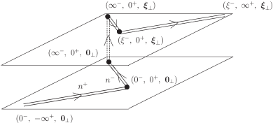
Figure 2: The integration contour associated with the additional soft counter term.

[Note that the result does not depend on the particular choice of the vector $l_{\perp}$.] The introduction of the soft factor $R$ is necessitated by the demand to cancel undesirable mixed rapidity divergences arising in the calculations with light-like quantities Col08 ; JMY04 ; CH00 ; Hau07 ; CM04 ; CS07 ; CS08 . Indeed, we have shown in CS07 ; CS08 , using the light-cone gauge with the advanced, retarded, or principal-value prescription, that the anomalous dimension entailed by the UV-divergences of graph (c) in Fig. 3 (generated by the soft factor $R$), cancels the corresponding contribution of the TMD PDF, given by graph (a) in the same figure. On the other hand, pure rapidity divergences still appear in the UV-finite graphs with real-gluon emissions—see Fig. 4.

In this section, we shall show that the use of the ML-gauge allows one to avoid rapidity divergences in the anomalous dimension of the TMD PDF, while preserving at the same time the validity (and gauge invariance) of definition (27). Nevertheless, the rapidity divergences, disentangled from the UV-singularities, are still present in the ML-gauge as well. The resummation of them should be pursued by means of the evolution equation which is analogous to the Collins-Soper one. This issue will be considered elsewhere separately.

Up to the LO in powers of $\alpha_{s}$, the TMD PDF (27) can be cast in the form

$$f_{q/q}^{\rm LO}=f^{(0)}+f^{(1)}+O(\alpha_{s}^{2})\ \ ,\ \ f^{(1)}=f_{\rm virt.}^{(1)}+f_{\rm real}^{(1)}\ ,$$ (30)

where we have separated virtual (see Fig. 3) from real (see Fig. 4) corrections (labeled accordingly). The real-gluon terms $f_{\rm real}^{(1)}$ do not contain UV divergences and hence will not be considered any further. In the tree approximation, one has

$$f_{q/q}^{(0)}(x,\mbox{\boldmath$k$}_{\perp}) = \frac{1}{2}\int\frac{d\xi^{-}d^{2}\mbox{\boldmath$\xi_{\perp}$}}{2\pi(2\pi)^{2}}{\rm e}^{-ik^{+}\xi^{-}+i{\mbox{\footnotesize\boldmath$k_{\perp}$}}\cdot\mbox{\footnotesize\boldmath$\xi_{\perp}$}}\langle p|\bar{\psi}(\xi^{-},\mbox{\boldmath$\xi_{\perp}$})\gamma^{+}\psi(0^{-},\mbox{\boldmath$0_{\perp}$})|p\rangle$$ (31)

$$= \delta(1-x)\delta^{(2)}(\mbox{\boldmath$k$}_{\perp})\ .$$

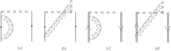
Figure 3: Virtual one-loop gluon contributions (curly lines) to the UV-divergences of the TMD PDF in the light-cone gauge—graphs (a) and (b). The graphs (c) and (d) are corresponding contributions originating from the soft factor $R$. Double lines denote gauge links. The vertical ones represent the transverse gauge links. The Hermitian conjugated diagrams are not shown.

The extraction of the UV-singular part of $f^{(1)}$ proceeds along the lines of our previous works, described in CS07 ; CS08 . In order to isolate the leading-order UV-divergent terms, one has to consider the virtual one-gluon contributions depicted in the diagrams of Fig. 3. These diagrams amount to

$$f_{\rm virt.}^{(1)}=\delta(1-x)\delta^{(2)}(\mbox{\boldmath$k$}_{\perp})\ \Sigma^{(1)}_{\rm virt.}(p)\ \gamma^{+}\ ,$$

so that $\Sigma^{(1)}_{\rm virt.}=\Sigma^{(a)}+\Sigma^{(b)}$. The quark self-energy diagram $(a)$ gives (in dimensional regularization with $\omega=4-2\epsilon$)

$${\Sigma}^{(a)}(p,\alpha_{s};\mu,\epsilon)={\Sigma}^{(a)}_{\rm Feynman}+{\Sigma}^{(a)}_{\rm ML}=-g^{2}C_{\rm F}\mu^{2\epsilon}\ \int\!\frac{d^{\omega}q}{(2\pi)^{\omega}}\frac{\gamma_{\mu}(\hat{p}-\hat{q})\gamma_{\nu}}{(p-q)^{2}(q^{2}+i0)}\ d^{\mu\nu}_{\rm ML}(q)\frac{i\hat{p}}{p^{2}}$$ (32)

with

$$d^{\mu\nu}_{\rm LC}(q)=g^{\mu\nu}-\frac{q^{\mu}(n^{-})^{\nu}+{q^{\nu}(n^{-})^{\mu}}}{[q^{+}]_{\rm ML}}\ .$$ (33)

After some standard calculations, one has for the prescription-independent $g_{\mu\nu}$ (“Feynman”) term

$${\Sigma}^{(a)}_{\rm Feynman}(p,\alpha_{s},\mu,\epsilon) = -g^{2}C_{\rm F}\mu^{2\epsilon}\ \int\!\frac{d^{\omega}q}{(2\pi)^{\omega}}\frac{\gamma_{\mu}(\hat{p}-\hat{q})\gamma^{\mu}}{(p-q)^{2}(q^{2}+i0)}\ \frac{i\hat{p}}{p^{2}}$$ (34)

$$= -\frac{\alpha_{s}}{4\pi}C_{\rm F}\ \Gamma(\epsilon)\left(-4\pi\frac{\mu^{2}}{p^{2}}\right)^{\epsilon}\frac{\Gamma(1-\epsilon)\Gamma(2-\epsilon)}{\Gamma(2-2\epsilon)}\ .$$

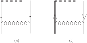
Figure 4: Real gluon contributions (curly lines) to the TMD PDF in the light-cone gauge using the ML pole prescription (“ML gauge”). Double lines denote gauge links. The Hermitian conjugated diagrams are not shown.

The evaluation of the ML-dependent part

$${\Sigma}^{(a)}_{\rm ML}(p,\alpha_{s},\mu;\epsilon)=g^{2}C_{\rm F}\mu^{2\epsilon}\!\int\!\frac{d^{\omega}q}{(2\pi)^{\omega}}\frac{1}{(p-q)^{2}(q^{2}+i0)}\left[\frac{\hat{q}(\hat{p}-\hat{q})\gamma^{+}}{[q^{+}]_{\rm ML}}+\frac{\gamma^{+}(\hat{p}-\hat{q})\hat{q}}{[q^{+}]_{\rm ML}}\right]\frac{i\hat{p}}{p^{2}}$$ (35)

is more involved. After the transformation of the numerator, one gets

$${\Sigma}^{(a)}_{\rm ML}=g^{2}C_{\rm F}\mu^{2\epsilon}\ \int\!\frac{d^{\omega}q}{(2\pi)^{\omega}}\left[(\hat{p}\gamma_{\mu}\gamma^{+}+\gamma^{+}\gamma_{\mu}\hat{p})\frac{(p-q)^{\mu}}{(p-q)^{2}}-2\gamma^{+}\right]\frac{1}{(q^{2}+i0)[q^{+}]_{\rm ML}}\frac{i\hat{p}}{p^{2}}\ .$$ (36)

Let us first consider the following integral BR05 ; CDL83 :

$$\int\!\frac{d^{\omega}q}{(2\pi)^{\omega}}\frac{1}{[q^{+}]_{\rm ML}}\ \frac{1}{q^{2}(p-q)^{2}}\ = \int\!d\alpha\int\!d\beta\ \int\!\frac{d^{\omega}q}{(2\pi)^{\omega}}\frac{\hbox{e}^{i(\alpha q^{2}+\beta(p-q)^{2})}}{[q^{+}]_{\rm ML}}$$ (37)

$$= -\frac{i}{(4\pi)^{\omega/2}}\frac{\Gamma(\epsilon)}{p^{+}(-p^{2})^{\epsilon}}\frac{1}{\epsilon}\ \left[\frac{\Gamma^{2}(1-\epsilon)}{\Gamma(1-2\epsilon)}-1\right]\ ,$$

where we have assumed that the direction of the momentum $p$ of the struck quark is purely longitudinal, i.e., $\mbox{\boldmath$p$}_{\perp}=0$. At first sight, the above expression seems to have a double pole in $1/\epsilon$. Expanding the $\Gamma$ functions, one, however, finds that Eq. (37) is finite and does not contribute any UV singularities. In contrast, the integral with $q^{\mu}$ in the numerator is UV singular. In order to calculate it, we use the $\alpha$-representation to obtain

$$\int\!\frac{d^{\omega}q}{(2\pi)^{\omega}}\frac{q^{\mu}}{[q^{+}]_{\rm ML}}\ \frac{1}{q^{2}(p-q)^{2}}\ =-\frac{i}{2}\ \int_{0}^{1}\!\frac{dx}{x}\ \int_{0}^{\infty}\!dL\ \hbox{e}^{ixLp^{2}}\ \frac{\partial}{\partial p_{\mu}}\int\!\frac{d^{\omega}q}{(2\pi)^{\omega}}\frac{\hbox{e}^{i(Lq^{2}-2xL(p\cdot q))}}{[q^{+}]_{\rm ML}}\ .$$ (38)

Taking into account that

$$\frac{\partial}{\partial p_{\mu}}\frac{1}{p^{+}}=\frac{(n^{-})^{\mu}}{(p^{+})^{2}}\ ,$$ (39)

one finds that there are two parts: one proportional to $(n^{-})^{\mu}$, the other to $p^{\mu}$. The first part vanishes in the final result by virtue of $(n^{-})^{\mu}(n^{-})_{\mu}=0$. Evaluating the second part, using (37), gives

$$\int\!\frac{d^{\omega}q}{(2\pi)^{\omega}}\frac{q^{\mu}}{[q^{+}]_{\rm ML}}\ \frac{1}{q^{2}(p-q)^{2}}\ =-\frac{i}{(4\pi)^{\omega/2}}\frac{p^{\mu}\ \Gamma(\epsilon)}{p^{+}(-p^{2})^{\epsilon}}\ \frac{\Gamma^{2}(1-\epsilon)}{\Gamma(2-2\epsilon)}\ .$$ (40)

This integral contains a single $1/\epsilon$-pole and thus contributes to the leading UV-singularity. In total, we find for diagram (a)

$${\Sigma}^{(a)}(p,\alpha_{s};\mu,\epsilon)={\Sigma}^{(a)}_{\rm Feynman}+{\Sigma}^{(a)}_{\rm ML}=-\frac{\alpha_{s}}{4\pi}C_{\rm F}\ \Gamma(\epsilon)\left(-4\pi\frac{\mu^{2}}{p^{2}}\right)^{\epsilon}\frac{\Gamma^{2}(1-\epsilon)}{\Gamma(2-2\epsilon)}\left[(1-\epsilon)-4\right]\ .$$ (41)

Extracting the UV divergent terms in the $\overline{\rm MS}$-scheme, one gets (after adding the conjugated diagrams):

$${\Sigma}_{(a)}^{\rm UV}(p,\alpha_{s},\mu,\epsilon)=-\frac{\alpha_{s}}{4\pi}C_{\rm F}\left[\frac{1}{\epsilon}(1-4)-\gamma_{E}+4\pi\right]=-\frac{3\alpha_{s}}{4\pi}C_{\rm F}\left[\frac{1}{\epsilon}-\gamma_{E}+4\pi\right]\ .$$ (42)

This expression makes it apparent that in the ML-gauge the UV-divergent part of the TMD PDF (as well as the finite one) do not contain any extra terms of the form $\ln p^{+}$ which could be related to a cusped contour—in contrast to the results obtained using $q^{-}$-independent prescriptions CS07 ; CS08 . Moreover, one sees that there is no imaginary term, as well, which is, however, necessary in order to reproduce the result in covariant gauges. We shall show next how this term arises due to the transverse gauge link at light-cone infinity.

IV Contribution of the transverse gauge link at light-cone infinity

The path-ordered composite transverse gauge link at light-cone infinity reads

$${\cal P}\exp\left[+ig\int_{0}^{\infty}\!d\tau\mbox{\boldmath$l$}^{\perp}\cdot\mbox{\boldmath$A$}^{\perp}(\infty^{-},0^{+};\mbox{\boldmath$l$}_{\perp}\tau+\mbox{\boldmath$\xi$}_{\perp})\right]\ {\cal P}\exp\left[-ig\int_{0}^{\infty}\!d\tau\mbox{\boldmath$l$}^{\perp}\cdot\mbox{\boldmath$A$}^{\perp}(\infty^{-},0^{+};\mbox{\boldmath$l$}_{\perp}\tau)\right]\ .$$ (43)

In leading non-vanishing order, the corresponding diagram $(b)$ in Fig. 3 yields

$${\Sigma}_{\rm ML}^{(b)}(p,\mu,g;\epsilon) = -g^{2}C_{\rm F}\mu^{2\epsilon}\int\!\frac{d^{\omega}q^{\prime}}{(2\pi)^{\omega}}\!\int\!\frac{dq^{+}}{2\pi}\hbox{e}^{-iq^{+}\infty^{-}}\!\!\int\!\frac{d^{2}q_{\perp}}{(2\pi)^{2}}\ \mbox{\boldmath$l$}^{\perp}\cdot\langle 0|A^{\mu}(q)\mbox{\boldmath$A$}^{\perp}(q^{\prime})|0\rangle$$ (44)

$$\times\frac{i}{(\mbox{\boldmath$q$}^{\perp}\cdot\mbox{\boldmath$l$}^{\perp})+i0}\ \frac{\gamma^{+}(\hat{p}-\hat{q})}{(p-q)^{2}}\ .$$

To evaluate this expression, we employ the gluon propagator in the ML-gauge which corresponds to the correlation function between the longitudinal and the transverse gluon fields:

$$\langle 0|A^{\mu}(q)\mbox{\boldmath$A$}^{\perp}(q^{\prime})|0\rangle=-\frac{\mbox{\boldmath$q$}^{\perp}n^{-\mu}}{(q^{2}+i0)[q^{+}]_{\rm ML}}(-i)(2\pi)^{4}\delta^{(4)}(q+q^{\prime})\ .$$ (45)

Using the explicit form of the ML-gauge field at light-cone infinity (cf. Eq. (25)), the transverse integral can be rewritten in the form

$$\int_{0}^{\infty}\!d\tau\mbox{\boldmath$l$}^{\perp}\cdot\mbox{\boldmath$A$}^{\perp}(\infty^{-},0^{+};\mbox{\boldmath$l$}_{\perp}\tau)=\int\!\frac{dq^{+}}{2\pi}\hbox{e}^{-iq^{+}\infty^{-}}\int\!\frac{d^{2}q_{\perp}}{(2\pi)^{2}}\ \mbox{\boldmath$l$}^{\perp}\cdot\mbox{\boldmath$A$}^{\perp}(q)\frac{i}{(\mbox{\boldmath$q$}^{\perp}\cdot\mbox{\boldmath$l$}^{\perp})+i0}\ .$$ (46)

Taking into account that

$$\frac{1}{[q^{+}]_{\rm ML}}=\frac{q^{-}}{q^{+}q^{-}+i0}=q^{-}\left[{\cal P}\frac{1}{q^{+}q^{-}}-i\pi\delta(q^{+}q^{-})\right]\ ,$$ (47)

and using the equation (valid in the sense of distributions, see, e.g., Ref. BJY03 )

$$\frac{\hbox{e}^{-iq^{+}\infty^{-}}}{q^{+}+i0}=-2\pi i\ \delta(q^{+})\ ,$$ (48)

one can change variables in the $\delta$-function to obtain

$${\Sigma}_{\rm ML}^{(b)}(p,\mu,g;\epsilon)=-g^{2}C_{\rm F}\mu^{2\epsilon}2\pi i\int\!\frac{d^{\omega}q}{(2\pi)^{\omega}}\delta(q^{+})\ \frac{\gamma^{+}(\hat{p}-\hat{q})}{(p-q)^{2}\ q^{2}}\ .$$ (49)

Finally, by taking the sum of the UV-divergent $(a)$ and $(b)$ contributions (Fig. 3), we find

$${\Sigma}^{(a+b)\rm UV}_{\rm ML}(p,\mu,\alpha_{s};\epsilon)=-\frac{\alpha_{s}}{\pi}\ C_{\rm F}\ \Bigg{\{}\frac{1}{\epsilon}\left[\frac{1}{4}-\frac{\gamma^{+}\hat{p}}{2p^{+}}\left(1-\frac{i\pi}{2}\right)\right]-\gamma_{E}+4\pi\Bigg{\}}$$ (50)

which yields ($\gamma^{+}\hat{p}\gamma^{+}/2p^{+}=\gamma^{+}$)

$${\Sigma}^{(a+b)\rm UV}_{\rm ML}(p,\mu,\alpha_{s};\epsilon)=\frac{\alpha_{s}}{\pi}\ C_{\rm F}\ \left[\frac{1}{\epsilon}\left(\frac{3}{4}+\frac{i\pi}{2}\right)-\gamma_{E}+4\pi\right]\ .$$ (51)

This result resembles what one finds in covariant gauges. After including the mirror contribution to graph (b) in Fig. 3, one obtains the following expression

$${\Sigma}^{(a+b)\rm UV}_{\rm ML}(p,\mu,\alpha_{s};\epsilon)=\frac{\alpha_{s}}{\pi}\ C_{\rm F}\ \left[\frac{1}{\epsilon}\frac{3}{4}-\gamma_{E}+4\pi\right]\ ,$$ (52)

which is analogous to Eq. (42) and does not contain an imaginary part. Hence, for the Mandelstam-Leibbrandt pole prescription, the UV-singular parts of the TMD PFDs reproduce the result obtained in a covariant gauge, where there are no effects from artifacts of gauge-contour obstructions (one encounters when using the light-cone gauge in association with the advanced, retarded, or principal-value prescription).

V Evaluation of the soft factor

To complete our arguments, we have now to verify whether the modified definition (27), proposed in CS07 ; CS08 using a light-cone gauge in conjunction with the advanced, retarded, or PV prescription, remains valid in the ML-gauge as well. The main ingredient of this definition is a soft factor which was introduced in order to compensate the extra (mixed) UV divergence and associated anomalous dimension originating from a cusped contour. However, the latter are absent in the ML-gauge, as we have shown above. Therefore, we have to demonstrate that the soft factor in this case does not jeopardize Eq. (27). In leading order, the UV singularities of the soft factor are generated by the self-energy of the light-like gauge link and the one-gluon exchanges between the light-like and the transverse gauge link (see diagrams $(c)$ and $(d)$ in Fig. 3, respectively). Thus, one has

$$\Phi_{\rm soft}^{\rm LO}=\Phi_{\rm soft}^{(0)}+\Phi_{\rm soft}^{(1)}+O(\alpha_{s}^{2})\ \ ,$$ (53)

$$\Phi_{\rm soft}^{(0)}=1\ \ ,\ \ \Phi_{\rm soft}^{(1)}=\Phi_{\rm soft-virt}^{(1)}+\Phi_{\rm soft-real}^{(1)}\ ,\ \Phi_{\rm soft-virt}^{(1)}=\Phi_{\rm soft-virt}^{(c)}+\Phi_{\rm soft-virt}^{(d)}$$

$$\Phi_{\rm soft-virt}^{(c)} = ig^{2}\mu^{2\epsilon}C_{\rm F}\ u_{\mu}u_{\nu}\int_{0}^{\infty}d\sigma\int_{0}^{\sigma}d\tau\int\!\frac{d^{\omega}q}{(2\pi)^{\omega}}\frac{\hbox{e}^{-iq\cdot u(\sigma-\tau)}}{q^{2}+i0}\left(g^{\mu\nu}-\frac{q^{\mu}n^{-\nu}+q^{\nu}n^{-\mu}}{[q^{+}]}\right)\$$ (54)

$$= 2ig^{2}\mu^{2\epsilon}C_{\rm F}\ \int_{0}^{\infty}d\sigma\int_{0}^{\sigma}d\tau\int\!\frac{d^{\omega}q}{(2\pi)^{\omega}}\frac{\hbox{e}^{-iq^{-}(\sigma-\tau)}}{2q^{+}q^{-}-\mbox{\boldmath$q$}_{\perp}^{2}+i0}\frac{q^{-}}{q^{+}+i0q^{-}}\ ,$$

where the vector $u_{\mu}$ is chosen to be light-like: $u_{\mu}=(p^{+},0^{-},\mbox{\boldmath$0$}_{\perp})$. Due to the relative positions of the poles in the Feynman and the ML-denominators, this integral is zero BKKN93 , i.e., both poles are on the same side of the $q^{+}$-axis:

$$\Phi_{\rm soft-virt}^{(c)\rm ML}=0\ .$$ (55)

For the same reason, the contribution of diagram $(d)$ in Fig. 2 vanishes as well, entailing $\Phi_{\rm soft-virt}^{(d)\rm ML}=0$. On the other hand, the contribution arising from real gluons, $\Phi_{\rm soft-real}^{(1)}$, does not contain UV-singularities. Hence, $\Phi_{\rm soft}^{\rm LO}$ reduces to unity, excluding the appearance of any contribution to the anomalous dimension of the TMD PDF related to spurious rapidity divergences. This result validates Eq. (27) also for the case of the light-cone gauge with the ML-prescription.

Further, the anomalous dimension of the modified TMD PDF (27) coincides, therefore, with the anomalous dimension of the standard TMD PDF (cf. (5)) in the light-cone gauge with the ML-prescription. Consequently, the renormalization-group properties of the TMD PDF are controlled by the following evolution equation

$$\frac{1}{2}\mu\frac{d}{d\mu}\ f_{i/q}^{\rm mod}(x,\mbox{\boldmath$k_{\perp}$};\mu) =\int\!d^{2}\mbox{\boldmath$q$}_{\perp}\ \int_{x}^{1}\!\frac{dz}{z}\ P_{\perp}\left(\frac{x}{z},\mbox{\boldmath$q$}_{\perp},\alpha_{s}\right)\ f_{i/q}^{\rm mod}(z,\mbox{\boldmath$q$}_{\perp},\mu)\ ,$$

$$P_{\perp}\left(y,\mbox{\boldmath$q$}_{\perp},\alpha_{s}\right) =\gamma_{\rm ML}\ \delta(1-y)\ \delta^{(2)}(\mbox{\boldmath$k$}_{\perp}-\mbox{\boldmath$q$}_{\perp})+O(\alpha_{s}^{2})\ ,$$ (56)

where the anomalous dimension coincides with the standard expression, i.e.,

$$\gamma_{\rm ML}=-\frac{1}{2}\mu\frac{d}{d\mu}\ln\Sigma_{\rm ML}(\alpha_{s},\epsilon)=\frac{3}{4}\frac{\alpha_{s}}{\pi}\,C_{\rm F}+O(\alpha_{s}^{2})\ .$$ (57)

VI Conclusions

This work was devoted to the treatment of mixed rapidity divergences of fully gauge-invariant TMD PDFs when employing the light-cone gauge in conjunction with the Mandelstam-Leibbrandt pole prescription. To this end, we calculated the leading-order contributions to the TMD PDF ensuing from virtual gluon corrections. Exactly these terms contain the UV singularities of the TMD PDF and thereby entail its anomalous dimension. We have shown by explicit calculation at one loop that, in contrast to other popular pole prescriptions, like the advanced, retarded, or the principal-value one, the Mandelstam-Leibbrandt prescription possesses the important property that spurious mixed rapidity divergences, related to obstructions of the gauge contour, are absent. Correspondingly, the soft factor, we introduced in CS07 ; CS08 in order to ensure the cancelation of such artifacts to the anomalous dimension of the TMD PDF, reduces in this case to unity, thus preserving its validity.

Phenomenologically, the use of the ML pole prescription in the light-cone gauge will facilitate calculations of TMD PDFs in a factorized description of SIDIS cross sections because the contributions to the anomalous dimensions from gauge-contour obstructions in the Wilson lines of the TMD PDFs cancel out, making the insertion of a correcting soft factor superfluous right from the start. This is also reflected in the evolution behavior of the TMD PDFs which is controlled by the standard anomalous dimension one finds in a covariant gauge, where anomalous-dimension artifacts are manifestly absent because factorization is complete like in collinear factorization. These aspects and the practical analysis of their applications will be considered in more detail elsewhere.

References

• (1) J.C. Collins, Acta Phys. Pol. B 34 (2003) 3103.
• (2) A.V. Belitsky, A.V. Radyushkin, Phys. Rept. 418 (2005) 1.
• (3) J. Collins, PoS LC2008 (2008) 028 [arXiv:0808.2665 [hep-ph]].
• (4) G. Altarelli, G. Parisi, Nucl. Phys. B 126 (1977) 298.
• (5) J.C. Collins, D.E. Soper, Nucl. Phys. B 194 (1982) 445.
• (6) V.N. Gribov, L.N. Lipatov, Sov. J. Nucl. Phys. 15 (1972) 438 [Yad. Fiz. 15 (1972) 781; V.N. Gribov, L.N. Lipatov, Sov. J. Nucl. Phys. 15 (1972) 675 [Yad. Fiz. 15 (1972) 1218]; L.N. Lipatov, Sov. J. Nucl. Phys. 20 (1975) 94 [Yad. Fiz.  20 (1974) 181]; Y.L. Dokshitzer, JETP 46 (1977) 641 [Zh. Eksp. Teor. Fiz. 73 (1977) 1216].
• (7) J.C. Collins, D.E. Soper, Nucl. Phys. B193 (1981) 381; B213 (983) 545 (E).
• (8) X. Ji, F. Yuan, Phys. Lett. B 543 (2002) 66.
• (9) A.V. Belitsky, X. Ji, F. Yuan, Nucl. Phys. B 656 (2003) 165.
• (10) D. Boer, P.J. Mulders, F. Pijlman, Nucl. Phys. B667 (2003) 201.
• (11) J.C. Collins, T.C. Rogers, A.M. Stasto, Phys. Rev. D 77 (2008) 085009.
• (12) A. Bacchetta, D. Boer, M. Diehl, P.J. Mulders, JHEP 0808 (2008) 023.
• (13) I.O. Cherednikov, N.G. Stefanis, Phys. Rev. D 77 (2008) 094001.
• (14) I.O. Cherednikov, N.G. Stefanis, Nucl. Phys. B 802 (2008) 146.
• (15) X. Ji, J. Ma, F. Yuan, Phys. Rev. D 71 (2005) 034005.
• (16) J.C. Collins, F. Hautmann, Phys. Lett. B 472 (2000) 129.
• (17) F. Hautmann, Phys. Lett. B 655 (2007) 26.
• (18) J.C. Collins, A. Metz, Phys. Rev. Lett. 93 (2004) 252001.
• (19) A. Bassetto, Nucl. Phys. Proc. Suppl. 51C (1996) 281.
• (20) G. Leibbrandt, S.L. Nyeo, Phys. Lett. B 140 (1984) 417.
• (21) A. Bassetto, G. Heinrich, Z. Kunszt, W. Vogelsang, Phys. Rev. D 58 (1998) 094020.
• (22) S. Mandelstam, Nucl. Phys. B 213 (1983) 149.
• (23) G. Leibbrandt, Phys. Rev. D 29 (1984) 1699.
• (24) G. Curci, W. Furmanski, R. Petronzio, Nucl. Phys. B 175 (1980) 27.
• (25) A.A. Slavnov, S.A. Frolov, Theor. Math. Phys. 73 (1987) 1158 [Teor. Mat. Fiz. 73 (1987) 199].
• (26) A. Bassetto, M. Dalbosco, I. Lazzizzera, R. Soldati, Phys. Rev. D 31 (1985) 2012.
• (27) A. Bassetto, M. Dalbosco and R. Soldati, Phys. Rev. D 36 (1987) 3138.
• (28) G.P. Korchemsky, A.V. Radyushkin, Nucl. Phys. B 283 (1987) 342.
• (29) D.M. Capper, J.J. Dulwich, M.J. Litvak, Nucl. Phys. B 241 (1984) 463.
• (30) A. Bassetto, I.A. Korchemskaya, G.P. Korchemsky, G. Nardelli, Nucl. Phys. B 408 (1993) 62.