Abstract

We develop a technique to formulate quantum field theory on arbitrary network, based on different, randomly disposed sets of scattering’s. We define R-matrix of the whole network as a product of R-matrices attached to each of scattering nods. Then an action for a network in terms of fermionic fields is formulated, which allows to calculate the transition amplitudes as their Green functions. On so-called bubble and triangle diagrams it is shown that the method produces the same results as the one which uses the generalized star product. The approach allows to extend network models by including multiparticle interactions at the scattering nods.

LAPTH-1324/09

CERN-PH-TH/2009-041

1 Introduction

Special and growing attention is brought today to quantum graphs, that is networks of one dimension and thin quantum wires connected at nodes. If such an interest can easily be explained by the current developments in nano-scale technology, one may also note that this domain of research is particularly attractive as well for condensed matter physicists as for mathematical graph theory .

Different aspects of quantum field theory (QFT) have to be taken into account and developed for such a context of problem, with among others the behavior of fields at the junctions(vertices) of different edges. Up to now, it is the case of star graphs which has received special consideration and for which some significant results have been obtained. Such graphs are constituted by only one vertex connecting several edges, and can be seen as the fundamental parts of generic graphs. The case of a junction with three quantum wires has in particular been considered in the study of a one-dimensional electron gas [2, 3, 4, 5] with the technique of bosonisation naturally playing an essential role.

Meantime, the formulation of quantum scattering theory on a graph, based on the connection of self adjoint extensions of the Schrodinger operator and Hermitian symplectic forms, provided an explicit expression of the unitary scattering S-matrix formed by the reflection and transmission amplitudes and encoding the allowed boundary conditions at the vertices [6]. Moreover, in the works [6, 7, 8] different, but equivalent rules for obtaining the transmission and reflection amplitudes were given. One rule is based on the so called generalized star product. All rules are based on linear algebra and are relatively simple to apply. In particular they may easily be implemented for the purpose of numerical calculations.

Then, combining these last results with an algebraic field theoretical treatment for quantum integrable systems in (1+1) dimensions with a reflecting and transmitting impurity [9] allowed the authors of [10, 11, 12] to develop a general framework for constructing, via the so-called reflection-transmission or ”R-T” algebra, vertex operators from bosonic fields propagating freely in the bulk and interacting at the junction. After a detailed study of scale-invariant interactions, and an explicit determination of the critical points for a star graph with any number $n$ of edges, the four fermion bulk interaction could then be considered and the Tomonaga-Luttinger/Thirring model solved at such critical points. This result is finally used for determining the charge and spin transport as well as to establish a relationship between them, recovering and extending the previous results first obtained in [2], and later confirmed in [3, 4, 5].

Such interesting results urge on the study of more complex graphs representing more realistic situations, the rather obvious next step being the case of a network with more than one vertex, linked together by internal wires, and particularly configurations where closed loops are present. The simplest examples in this last case are the ”bubble diagram” (see below Fig.7) with two vertices related by two internal wires, and the ”triangle diagram” (see Fig.8) where three star graphs combine in such a way that each couple of vertices is connected by an internal line. In order to extend the previous formalism developed in [10, 11, 12], one can wonder whether the closed diagram made of several junction points, each one connected with an internal as well as one or more external wires, can be represented by an unique ”mega” vertex with the same external lines. This is one of the results of this paper, where an explicit construction of the scattering S-matrix relative to the ”mega” vertex is given in terms of the scattering S-matrix elements of the different vertices involved. At this point let us mention that direct computations of the final S-matrices have recently been performed in the case of a chain of impurities Ref.[13] as well as for closed loops Ref.[14]. A direct comparison of some of the results obtained by this last approach with ours can easily be done. But we must stress that the technique we are using is completely different from the one of Ref.[13, 14] and will allow us, as explained below, to propose an action formulation for models defined on a lattice associated to the considered network.

It is the extension of transfer matrix approach which is hereafter used to handle this problem. More precisely, to each of vertexes of the network we allocate a R-matrix, which is defined by the corresponding scattering S-matrix. Then we construct a product of all R-matrices of the network in an appropriate way defining mega-R-matrix. The resultant R-matrix defines an S-matrix of the whole network. This is one of main results of the paper. Then, using an approach first initiated in Ref.[15], we rewrite the R-matrix constructed for each star graph in terms of creation /annihilation operators ( representing the in/out-coming particles) and with coefficients directly related with S-matrix entries. The replacement of such operators by Grassmann-valued fields in 2-dim. space allows one to perform directly the product of such R-matrices, each associated to a different vertex connected to the next one by (at least) one internal line, and finally to reconstruct from the so-obtained transfer matrix the one mimicking the scattering of the ”mega” vertex containing the different connected junctions.

This technique, namely the transformation of the R-matrix into its coherent states basis in fermionic Fock-space allows to give an action formulation of the corresponding model on a lattice formed by the network. The explicit check of equivalence of the action formulation of network models on a basis of R-matrix with the star-product rules of calculations, earlier formulated in the paper [7], for so-called bubble and triangle diagrams is the another important result of this article. Note that the general proof of equivalence is given in [16].

The action formulation is a convenient way, if not the only, to investigate networks with large number N of vertices, or near the critical point, when one can develop an equivalent quantum field theory approach to the problem.

The importance of the action formulation of network models is hard to overestimate. It can be applied, for example, to the Chalker-Coddington (CC) phenomenological model [17] devoted to plateau-plateau transitions in quantum Hall effect. This approach to the CC model was developed in [18].

Let us at this point note that in Ref.[15] such a fermionization technique was also used for the formulation of lattice models in (2+1) dim. in connection with the 3D-Ising model. Applications for the construction of integrable models with staggered parameters have also been found [19]; see also [20] for more developments. Obviously, the direct connection between such lattice models and quantum graphs has to be exploited more deeply, and we will return to this point in our conclusion.

The paper is organized as follows. We start in Section 2 by considering the case of several impurities on a line. Then one easily notices that, by simply re-organizing the entries of the scattering S-matrix relative to each vertex, one gets transfer (T-) matrices such that their product, following the order of the different vertices along the line, provides one with a transfer matrix relating the external legs of the diagram: it is then a simple exercise to deduce, by an operation inverse to the previous one, a matrix which can be seen as the S-matrix of the ”mega” vertex of the diagram. Actually,the T-matrix associated to each vertex can be seen as the one particle sector of the extended XX-model R-matrix.

In the Section 3 we give the formulation of three-channel $R^{(3)}$-matrix in a standard matrix and operator forms. Then we pass to coherent state basis and present a simple expression of the $R^{(3)}$-matrix via three channel $S$-matrix. Then we formulate a problem of complicated networks and express total $R$-matrix as a product of its ingredient $R^{(2)}$ and $R^{(3)}$ matrices. This allows us also to give an action formulation for any complicated networks in via fermionic fields.

In Section 4 we apply our method to calculation of the so-called bubble diagram, while in Section 5 we present the calculations for the triangle vertex diagram and show, that corresponding mega-S-matrices coincides with the results obtained via star-product procedure given in [6, 7].

2 Two particle R-matrix

2.1 Connection of Transfer matrix with R-matrix

The act of the scattering of the particle on a potential center/impurity can be described by a 2x2 S-matrix of the form

$$\mid i>_{out}=S_{ij}\mid j>_{in},$$ (2.1)

where $i=1,2$ denote the number of channels: Figure 1 demonstrates this process.

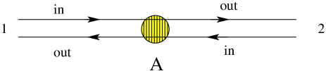
Figure 1: Two channel S-matrix.

The S-matrix consists of transmission $T_{12}(k),\;T_{21}(k)$ and reflection $R_{11}(k),\;R_{22}(k)$ amplitudes ( details can be found in [6, 13, 21].

$$S=\left(\begin{array}[]{cc}R_{11}(k)&T_{12}(k)\\ T_{21}(k)&R_{22}(k)\end{array}\right).$$ (2.4)

This two particle process can be described also by the transfer matrix which maps the states $\mid 1>_{in},\mid 1>_{out}$ on the left hand side of the scattering region $A$ to the $\mid 2>_{in},\mid 2>_{out}$ on the right hand side.

$$\left(\begin{array}[]{c}\mid 2>_{in}\\ \mid 2>_{out}\end{array}\right)=\left(\begin{array}[]{cc}\frac{1}{T_{12}(k)}&-\frac{R_{11}(k)}{T_{12}(k)}\\ -\frac{R_{11}(-k)}{T_{12}(-k)}&\frac{1}{T_{12}(-k)}\end{array}\right)\left(\begin{array}[]{c}\mid 1>_{out}\\ \mid 1>_{in}\end{array}\right)$$ (2.11)

In (2.11) the symmetry properties (unitarity, analyticity, consistency) of the $S$-matrix (2.4) have been taken into account. [6, 21, 13].

Since the transfer matrix maps the states on left hand side to the states on the right hand side of the scattering region the process of scattering on the multiple points will simply be described by the multiplication of the transfer matrices (see Fig.2).

Figure 2: Chain of two channel T-matrices representing a chain of equidistant impurities.

Continuously mapping the states from the left to the right on the Fig.2, we will have a product of transfer matrices

$$T^{(n)}=T_{n}T_{n-1}...T_{1},$$ (2.12)

the matrix elements defining final transmission $T^{(n)}_{12}(k)$ and reflection $R^{(n)}_{11}(k)$ amplitudes. This procedure of calculation of amplitudes is much simpler than calculations in S-matrix formalism, where we do not have local matrix multiplication but should deal with counting of non-local effects.

It appears that this transfer matrix can be considered as an one particle sector of the R-matrix of an XX-model. Namely, the standard form of the extended XX-model’s R-matrix can be represented as:

$$R_{XX}=\left(\begin{array}[]{cccc}-r_{22}&0&0&0\\ 0&1&-r_{21}&0\\ 0&r_{12}&r_{11}r_{22}-r_{12}r_{21}&0\\ 0&0&0&-r_{11}\end{array}\right),$$ (2.17)

where we denoted

$$R_{01}^{01} = 1,\;\;\qquad R_{10}^{10}=r_{11}r_{22}-r_{12}r_{21},\;\;R_{11}^{11}=-r_{22}$$

$$R_{00}^{00} = -r_{22},\;\;\qquad R_{01}^{10}=r_{12},\;\qquad\qquad R_{10}^{01}=-r_{21}.$$ (2.18)

Then, by use of unitary properties of the S-matrix (2.4) one easily can see, that the middle block of elements $R_{10}^{10},\;R_{01}^{01},\;R_{01}^{10},\;R_{10}^{01}$ will coincide with the transfer matrix (2.11) after dividing them on $-R_{00}^{00}$

$$T_{21}(k) = r_{11},\;\;T_{12}(k)=r_{22},\;\;$$

$$R_{11}(k) = r_{21},\;\;\quad R_{22}(k)=r_{12}.$$ (2.19)

Hence, the $r$-matrix elements are connected with the $S$-matrix ones as:

$$r=C\cdot S$$ (2.20)

with $C=\left(\begin{array}[]{cc}0&1\\ 1&0\end{array}\right)$, the numeration of spaces of the initial states differing in the R and T matrix formulations (compare Fig.1 with Fig.3 below).

Via Jordan-Wigner transformation, the R-matrix (2.17) can be represented as an operator consisting of fermionic creation/annihilation operators which act on a corresponding Fock space made of two quantum spaces (see Fig.3 below).

$$R^{(2)}_{12}:V_{1}\otimes V_{2}\rightarrow V_{1}\otimes V_{2}.$$ (2.21)

Now, let us introduce scalar fermions $c^{+}_{i},\;c_{i}$ in each linear space $V_{i},\;\;i=1,2$ forming a set of quantum states $|i>_{in/out}$. Defining the R-operator as

$$R^{(2)}_{12}=:e^{(-1)^{j}c_{i}^{+}(\delta_{ij}+r_{ij})c_{j}}:,$$ (2.22)

where we have normal ordering convention of operators in space $V_{1}$ and anti-normal ordering convention space $V_{2}$, one will obtain [22, 23]

$$R^{(2)}_{12} = R_{11}^{11}n_{1}n_{2}+R_{00}^{00}\bar{n}_{1}\bar{n}_{2}+R_{10}^{10}n_{1}\bar{n}_{2}$$ (2.23)

$$+ R_{01}^{01}\bar{n}_{1}n_{2}+R_{10}^{01}c^{+}_{1}c_{2}+R_{01}^{10}c^{+}_{2}c_{1},$$

where $n=c^{+}_{i}c_{i},\;\;i=1,2$ is the particle number operator and $\bar{n}_{i}=1-n_{i}$.

2.2 Chain of Equidistant Impurities

The transfer matrix approach allows to analyze very easily a chain of scattering centers/impurities and to calculate the transmission/reflection amplitudes. In this section we will explicit such a calculation by considering a chain of equidistant, identical impurities.

For such a purpose, we start by defining the local transfer matrix $T_{i}$ at the chain point $i$, with $i=1,...,n$ by translating the transfer matrix $T_{0}$ defined by the formula (2.11) at the point zero via translation operator

$$W_{i}=\left(\begin{array}[]{cc}e^{ikx_{i}}&0\\ 0&e^{-ikx_{i}}\end{array}\right)$$ (2.26)

as $T_{i}=W_{i}^{-1}T_{0}W_{i}$. Then the final transfer matrix appears as the product of the different local transfer matrices $T_{i}$:

$$T^{(n)}=T_{n}T_{n-1}\dots T_{1}=W_{n}^{-1}(T_{0}W)^{n}W^{-1}W_{1},$$ (2.27)

where $W=W_{i+1}W_{i}^{-1}$ is constant due to equidistant position of impurities $d=x_{i+1}-x_{i}=const$.

We need to calculate $T^{(n)}$. In order to reach this goal one can diagonalize the matrix $T_{0}W$ with the help of an unitary matrix $U$:

$$T^{(n)}=W_{n}^{-1}U(T_{0}W)^{n}_{diagonal}U^{+}W^{-1}W_{1}$$ (2.28)

The eigenvalues and eigenvectors of $T_{0}W$ can be obtained via:

$$\left(\begin{array}[]{cc}\frac{e^{ikd}}{T_{12}(k)}&-\frac{R_{11}(k)e^{-ikd}}{T_{12}(k)}\\ -\frac{R_{11}(-k)e^{ikd}}{T_{12}(-k)}&\frac{e^{-ikd}}{T_{12}(-k)}\end{array}\right)\left(\begin{array}[]{c}u_{\pm}\\ v_{\pm}\end{array}\right)=\lambda_{\pm}\left(\begin{array}[]{c}u_{\pm}\\ v_{\pm}\end{array}\right),$$ (2.35)

where eigenvalues $\lambda_{\pm}$ easily can be found with the characteristic equation:

$$\lambda^{2}-\lambda\left(\frac{e^{ikd}}{T_{12}(k)}+\frac{e^{-ikd}}{T_{12}(-k)}\right)+1=0.$$ (2.36)

Defining

$$\alpha(k)=ArcCosh\left[\frac{1}{2}\left(\frac{e^{ikd}}{T_{12}(k)}+\frac{e^{-ikd}}{T_{12}(-k)}\right)\right]$$ (2.37)

one can represent eigenvalues in a form

$$\lambda_{\pm}=e^{\pm\alpha(k)}.$$ (2.38)

After some more algebra, one gets for $T^{(n)}$:

$$T^{(n)}=\left(\begin{array}[]{cc}\frac{\sinh(n\alpha)}{\sinh(\alpha)}\frac{1}{T_{12}(k)}e^{ik(n-1)d}&-\frac{\sinh(n\alpha)}{\sinh(\alpha)}\frac{R_{11}(k)}{T_{12}(k)}e^{-ik(2x_{1}+(n-1)d)}\\ -\frac{\sinh((n-1)\alpha)}{\sinh(\alpha)}e^{ik(n-2)d}&\\[14.22636pt] -\frac{\sinh(n\alpha)}{\sinh(\alpha)}\frac{R_{11}(-k)}{T_{12}(-k)}e^{ik(2x_{1}+(n-1)d)}&\frac{\sinh(n\alpha)}{\sinh(\alpha)}\frac{1}{T_{12}(-k)}e^{-ik(n-1)d}\\ &-\frac{\sinh((n-1)\alpha)}{\sinh(\alpha)}e^{-ik(n-2)d}\end{array}\right).$$ (2.43)

Note that, in the case of only one impurity, i.e. n=1 and d=0, one directly recovers the T-matrix defined in Eq. (2.3) - as it should be.

2.3 Fermionic Coherent States

In this subsection we will define fermionic coherent states which are very instrumental in constructing of action/Lagrangian formulation of network models [15]. They form another basis of the linear space of the quantum states, giving the possibility to express the matrix elements of the R-matrix via Grassmann variables.

By definition, fermionic coherent/anticoherent states are eigenstates of fermion creation/annihilation operators $c,c^{+}$. Since the operators $c,c^{+}$ have anti-commuting properties, their eigenvalues cannot be ordinary numbers. They will be Grassmann variables satisfying the following properties:

$$\psi\psi = \bar{\psi}\bar{\psi}=0,\qquad\qquad\psi\bar{\psi}=-\bar{\psi}\psi,$$

$$\int d\psi = \int d\bar{\psi}=0,\qquad\int d\psi\psi=\int d\bar{\psi}\bar{\psi}=1.$$ (2.44)

With the help of these variables, let us define a coherent state:

$$\mid\psi\rangle=e^{-\psi c^{+}}\mid 0\rangle,\qquad\qquad\langle\bar{\psi}\mid=\langle 0\mid e^{-c\bar{\psi}},$$ (2.45)

as being an eigenstate of the annihilation operator $c$ with the eigenvalue $\psi$:

$$c\mid\psi\rangle=\psi\mid\psi\rangle\qquad\qquad\langle\bar{\psi}\mid c^{+}=\langle\bar{\psi}\mid\bar{\psi}.$$ (2.46)

Correspondingly, the anti-coherent state

$$\mid\bar{\psi}\rangle=(c^{+}-\bar{\psi})\mid 0\rangle,\qquad\qquad\langle\psi\mid=\langle 0\mid(c+\psi),$$ (2.47)

is an eigenstate of the creation operator $c^{+}$ with the eigenvalue $\bar{\psi}$:

$$c^{+}\mid\bar{\psi}\rangle=\bar{\psi}\mid\bar{\psi}\rangle\qquad\qquad\quad\;\langle\psi\mid c=-\langle\psi\mid\psi.$$ (2.48)

By use of the relations (2.3), it is straightforward to check that we get the following normalization:

$$\langle\bar{\psi}\mid\psi\rangle=e^{\bar{\psi}\psi}\qquad\qquad\langle\psi\mid\bar{\psi}\rangle=e^{\bar{\psi}\psi}$$ (2.49)

and the completeness relations:

$$\int d\bar{\psi}d\psi\mid\psi\rangle\langle\bar{\psi}\mid e^{\psi\bar{\psi}}=1,\qquad\int d\bar{\psi}d\psi\mid\bar{\psi}\rangle\langle\psi\mid e^{\psi\bar{\psi}}=1$$ (2.50)

for the coherent and anti-coherent states respectively.

The coherent states are forming a new basis in the two dimensional Fock space of fermions, where it becomes very easy to calculate the matrix elements of any functional in the operators $c,c^{+}$ written in a normal/anti-normal ordered form. In particular, it is straightforward to find out that, for any normal ordered operator $:F(c^{+},c):$

$$\langle\bar{\psi}\mid:F(c^{+},c):\mid\psi\rangle=F(\bar{\psi},\psi)e^{\bar{\psi}\psi}$$ (2.51)

while for an anti-normal ordered operator:

$$\langle\psi\mid:F(c^{+},c):\mid\bar{\psi}\rangle=F(\bar{\psi},-\psi)e^{\bar{\psi}\psi}.$$ (2.52)

Note also that the kernel $F(\bar{\psi},\psi)$ of two operators $:F(c^{+},c):=:F_{1}(c^{+},c)::F_{2}(c^{+},c):$ reads:

$$F(\bar{\psi},\psi)=\int d\bar{\chi}d\chi e^{-\bar{\chi}\chi}F_{1}(\bar{\psi},\chi)F_{2}(\bar{\chi},\psi).$$ (2.53)

We will use this relation extensively below.

The R-operator (2.23) has a very simple form in the coherent state basis. Introducing coherent/anti-coherent states $\bar{\psi}^{\prime}_{1},\;\psi_{1},\;\bar{\psi}_{2},\;\psi^{\prime}_{2}$ in the spaces $V_{1}/V_{2}$ correspondingly defined by formulas (2.45)/(2.47), one obtains for the matrix elements $\langle\psi^{\prime}_{2},\bar{\psi}^{\prime}_{1}\mid R\mid\;\psi_{1},\bar{\psi}_{2}\rangle$of the R-operator:

$$\langle\psi^{\prime}_{2},\bar{\psi}^{\prime}_{1}\mid R\mid\;\psi_{1},\bar{\psi}_{2}\rangle = e^{-r_{11}\bar{\psi}_{1}^{\prime}\psi_{1}-r_{22}\bar{\psi}_{2}\psi_{2}^{\prime}-r_{12}\bar{\psi}_{1}^{\prime}\psi_{2}^{\prime}-r_{21}\bar{\psi}_{2}\psi_{1}}$$ (2.54)

$$= e^{-\bar{\psi}_{i}(CS)_{ij}\psi_{j}}.$$

In order to make a correspondence with the notations on Fig.1, where the left hand states are marked with index 1, while right hand states are marked by 2, we redefine $\psi_{1}=\eta_{1},\bar{\psi^{\prime}}_{1}=\bar{\eta}_{2},\psi^{\prime}_{2}=\eta^{\prime}_{2},\bar{\psi}_{2}=\bar{\eta^{\prime}}_{1}$ and obtain for the $R$-matrix the expression

$$\langle\eta^{\prime}_{2},\bar{\eta}_{2}\mid R\mid\;\eta_{1},\bar{\eta^{\prime}}_{1}\rangle = e^{-\bar{\eta}_{i}S_{ij}\eta_{j}}.$$ (2.55)

Hereafter, we shall use $R$-matrices in this last formulation like (2.55).

Graphically, the R-operator in the coherent state basis can be represented as in Fig.3, where it becomes clear that the S-matrix parameters are merely hopping parameters.

Note that, in getting formula (2.54) we have used formulas (2.51-2.52) and (2.22).

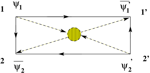
Figure 3: Convenient representation of two-channel R-matrix as an quadrangle where the sides are hopping links of fermions.

3 Three particle R-matrix

3.1 Three particle S-matrix

In this Section we will define the three particle R-matrix connected to the corresponding three particle S-matrix. The main problem that we would like to solve is the following. Usually, in order to describe the scattering of three particles we define a three particle S-matrix. But then it is very hard to make calculations in a situation when of a network with multiple scattering points. The problem stands in non-local rules of the S-matrix multiplications. The situation is totally different if we have to deal with multiplication of R-matrices. Then we have local multiplication rules of the tensorial type allowing to handle complicated problems with networks.

We will start from the three particle of S-matrix and define a corresponding R-matrix in the next section.

So, let us consider three channels where the incoming and outgoing states are marked as $\mid i>_{in}$ and $\mid i>_{out},\;\;(i=1,2,3)$ respectively. In a way similar to the two particle case (2.1), the three particle S-matrix is an matrix mapping incoming states to outgoing ones:

$$\mid i>_{out}=S_{ij}\mid j>_{in}$$ (3.56)

It is convenient to represent this scattering process by the vertex shown in Fig.3.

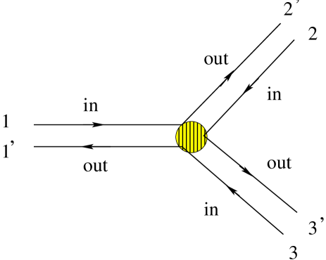
Figure 4: Three channel S-matrix/R-matrix.

3.2 Definition of Three Particle R-matrix

Up to this point the S-matrix was describing two channel scattering processes where 0,1,2 particles could participate. Now we introduce a three channel R-matrix containing information about 0,1,2,3 particle processes involved in the scattering.

For further convenience, we change the traditional notations of the states in the channel presented in the Fig.3 and make the re-numeration in accordance with Fig.4. Namely, let us change $|2^{\prime}\rangle\rightarrow|1^{\prime}\rangle$ and $|1^{\prime}\rangle\rightarrow|2^{\prime}\rangle$ and introduce the matrix:

$$r=CS,$$ (3.57)

where $S$ is the three channel S-matrix (3.56) and the matrix $C$

$$C=\left(\begin{array}[]{ccc}0&1&0\\ 1&0&0\\ 0&0&1\\ \end{array}\right).$$ (3.61)

ensures the re-numeration of the states according to Fig.4 and Fig.5.

The three particle R-matrix is a matrix/operator acting on the direct product of the three two dimensional linear spaces $V_{j},\;\;j=1,2,3$ ( Fig.5)

$$R_{123}:V_{1}\otimes V_{2}\otimes V_{3}\rightarrow V_{1}\otimes V_{2}\otimes V_{3}.$$ (3.62)

The dimension of $V$ spaces is defined by the number of incoming and outgoing states. In the simplest case it is two and we will consider this case in this article. Let us also define the basis states for the each space $V_{i}$ as $|0\rangle_{i}$ and $|1\rangle_{i}$.

Our aim is the definition of the R-matrix corresponding to the given S-matrix. Any R-matrix can be represented in three different bases of the linear spaces $V_{i},\;i=1,2,3$. The first, and the most popular one is an ordinary matrix form. In case of three particle, the R-matrix entries read $R_{\alpha\beta\gamma}^{\alpha^{\prime}\beta^{\prime}\gamma^{\prime}}$ where each index takes the values 0 and 1. As we will see below this notation is justified because it is connected with the particle (fermion) number in operator representation of the R-matrix. We will define and consider R-matrices corresponding to the processes with particle number conservation. The most general form of this type of R-matrix was defined in [20] and have a following form:

$$R=\left(\begin{array}[]{cccccccc}R_{000}^{000}&&&&&&&\\ &R_{001}^{001}&R_{010}^{001}&R_{100}^{001}&&&&\\ &R_{001}^{010}&R_{010}^{010}&R_{100}^{010}&&&&\\ &R_{001}^{100}&R_{010}^{100}&R_{100}^{100}&&&&\\ &&&&R_{011}^{011}&R_{101}^{011}&R_{110}^{011}&\\ &&&&R_{011}^{101}&R_{101}^{101}&R_{110}^{101}&\\ &&&&R_{011}^{110}&R_{101}^{110}&R_{101}^{110}&\\ &&&&&&&R_{111}^{111}\end{array}\right).$$ (3.71)

It is presented in a block-diagonal form, where each block corresponds respectively to the $0-,\;1-,\;2-,\;3-$ particle scattering: we interpret $|0\rangle,\;|1\rangle$ states as vacuum state and one particle state.

Each two dimensional space $V_{i},i=1,2,3$ can be realized as a Fock space of scalar fermions. This will allow to formulate the operator R-matrix in a fermionic space equivalent to the Jordan-Wigner transformation.

Let us introduce the creation/annihilation operators $c_{i},c^{+}_{i}$ of scalar fermions in each linear space $V_{i},\;i=1,2,3$ such as:

$$c_{i}|0\rangle_{i}=0,\quad c^{+}_{i}|0\rangle_{i}=|1\rangle_{i},$$

and consider the operator [20]:

$$R_{123}=:e^{(-1)^{j}c_{i}^{+}(\delta_{ij}+r_{ij})c_{j}}:$$ (3.72)

where the matrix elements $r_{ij}$ are forming the set of parameters of the model and are connected with S-matrix entries via formula (3.57) while the symbol :: means normal ordering of the operators in the space $i=1,3$ and anti-normal (hole) ordering for the fermions in $i=2$.

Expanding the exponent in the formula (3.72) and after some algebra one can obtain the following expression for the operator R-matrix:

$$R_{123} = R_{000}^{000}\bar{n}_{1}\bar{n}_{2}\bar{n}_{3}+R_{001}^{001}\bar{n}_{1}\bar{n}_{2}n_{3}+R_{010}^{010}\bar{n}_{1}n_{2}\bar{n}_{3}+R_{100}^{100}n_{1}\bar{n}_{2}\bar{n}_{3}$$ (3.73)

$$+ R_{011}^{011}\bar{n}_{1}n_{2}n_{3}+R_{101}^{101}n_{1}\bar{n}_{2}n_{3}+R_{110}^{110}n_{1}n_{2}\bar{n_{3}}+R_{111}^{111}n_{1}n_{2}n_{3}$$

$$+ (R_{001}^{010}c_{3}^{+}c_{2}+R_{001}^{010}c_{2}^{+}c_{3})\bar{n}_{1}+(R_{101}^{110}c_{3}^{+}c_{2}+R_{110}^{101}c_{2}^{+}c_{3})n_{1}$$

$$+ (R_{001}^{100}c_{3}^{+}c_{1}+R_{100}^{001}c_{1}^{+}c_{3})\bar{n}_{2}+(R_{011}^{110}c_{3}^{+}c_{1}+R_{110}^{011}c_{1}^{+}c_{3})n_{2}$$

$$+ (R_{010}^{100}c_{2}^{+}c_{1}+R_{100}^{010}c_{1}^{+}c_{2})\bar{n}_{3}+(R_{011}^{101}c_{2}^{+}c_{1}+R_{101}^{011}c_{1}^{+}c_{2})n_{3}$$

with

$$R_{111}^{111} = r_{11}r_{33}-r_{13}r_{31},\;R_{100}^{100}=r_{11}r_{22}-r_{12}r_{21},\;R_{001}^{001}=r_{33}r_{22}-r_{23}r_{32},$$

$$R_{010}^{010} = 1,\;\;R_{101}^{101}=-Det[(-1)^{j}r_{ij}],\;\;R_{110}^{110}=-r_{11},\;R_{000}^{000}=-r_{22},\;R_{011}^{011}=-r_{33},$$

$$R_{110}^{101} = r_{11}r_{23}-r_{13}r_{21},\;R_{101}^{110}=r_{12}r_{31}-r_{11}r_{32},\;R_{101}^{011}=r_{13}r_{32}-r_{33}r_{12},$$

$$R_{011}^{101} = r_{33}r_{21}-r_{23}r_{31},\;R_{100}^{001}=r_{22}r_{13}-r_{12}r_{23},\;R_{001}^{100}=r_{22}r_{31}-r_{21}r_{32},$$

$$R_{110}^{011} = r_{13},\;\;\hskip 42.67912ptR_{011}^{110}=r_{31},\;\;\hskip 42.67912ptR_{010}^{001}=-r_{23},\qquad\qquad$$

$$R_{001}^{010} = r_{32},\;\;\hskip 42.67912ptR_{100}^{010}=r_{12},\;\;\hskip 42.67912ptR_{010}^{100}=-r_{21}.$$ (3.74)

In the spaces $V_{i},\;i=1,2,3$ the creation-annihilation operators can be identified with $|\alpha\rangle_{i}\langle\alpha^{\prime}|$ as:

$$c_{i}=|0\rangle_{i}\langle 1|,\;\;\;\;c_{i}^{+}=|1\rangle_{i}\langle 0|,\;\;\;\;c_{i}^{+}c_{i}=|1\rangle_{i}\langle 1|,\;\;\;c_{i}c_{i}^{+}=|0\rangle_{i}\langle 0|.$$ (3.75)

Note that with this definition, each $V_{i}$ space acquires a grading: $|\alpha\rangle_{i}|\beta\rangle_{j}=(-1)^{p_{\alpha}p_{\beta}}|\beta\rangle_{j}|\alpha\rangle_{i},\;\;i\neq j$, where $p_{\alpha}=\alpha$ is the parity of the state $|\alpha\rangle$.

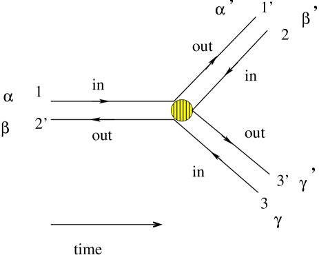
Figure 5: The R-matrix, attached to the S-matrix and defined by this picture, has the entries $R_{\alpha\beta\gamma}^{\alpha^{\prime}\beta^{\prime}\gamma^{\prime}}$

In this ket-bra language, the $R_{123}$-operator (3.72) can be represented via its matrix elements $R_{\alpha\beta\gamma}^{\alpha^{\prime}\beta^{\prime}\gamma^{\prime}}=\langle\gamma\beta\alpha\mid R\mid\alpha^{\prime}\beta^{\prime}\gamma^{\prime}\rangle$ in the following way:

$$R_{123} = R_{\alpha\beta\gamma}^{\alpha^{\prime}\beta^{\prime}\gamma^{\prime}}\Big{(}|\alpha\rangle_{1}|\beta\rangle_{2}|\gamma\rangle_{3}\Big{)}\Big{(}{}_{3}\langle\gamma^{\prime}|{}_{2}\langle\beta^{\prime}|{}_{1}\langle\alpha^{\prime}|\Big{)}$$

$$= R_{\alpha\beta\gamma}^{\alpha^{\prime}\beta^{\prime}\gamma^{\prime}}(-1)^{p_{\alpha}(p_{\alpha}+p_{\alpha^{\prime}})+p_{\beta^{\prime}}(p_{\gamma}+p_{\gamma^{\prime}})}\Big{(}|\alpha\rangle_{1}\langle\alpha^{\prime}|\Big{)}\Big{(}|\beta\rangle_{2}\langle\beta^{\prime}|\Big{)}\Big{(}|\gamma\rangle_{3}\langle\gamma^{\prime}|\Big{)}.$$

The operator $R_{123}$ has even parity, and for its non-zero matrix elements the relation $(-1)^{p_{\alpha}+p_{\beta}+p_{\gamma}+p_{\alpha^{\prime}}+p_{\beta^{\prime}}+p_{\gamma^{\prime}}}=1$ takes place.

The R-operator appears to have a very simple form in a coherent space representation defined by formulas (2.45-2.47). By using a coherent state basis (2.45) for the spaces $V_{1},V_{3}$, and an anti-coherent basis (2.47) for $V_{2}$ as well as the relations (2.51, 2.52), one can obtain a very transparent connection between the R- and the S-matrix. Namely:

$$R=e^{-\bar{\psi}_{i}r_{ij}\psi_{j}}=e^{-\bar{\eta}_{i}S_{ij}\eta_{j}},$$ (3.77)

where we have summation over $i,j=1,2,3$ and $\eta_{i}=\psi_{i},\;\bar{\eta}_{i}=C_{ij}\bar{\psi}_{j}$. According to the definitions in (3.57), the first equation in (3.77) corresponds to the Fig.5, the second one to the Fig.4, i.e $r_{ij}$ and $S_{ij}$ are the hopping parameters defined on the network of Fig.5 and Fig.4 respectively.

One needs also to define the $R_{123}$ operator with inverse orderings: hole-ordering and anti-coherent basis for the spaces $V_{1},V_{3}$, and normal ordering and coherent state basis for $V_{2}$. This will bring to the respective changes of the expressions of the matrix elements of $R^{(3)}$ written in terms of $r_{ij}$ matrix elements.

The connection of three particle $R^{(3)}$-matrix (3.57) with two particle one defined by (2.1) is very simple. Namely:

$$R_{\alpha\;\beta}^{(2)\alpha\prime\beta\prime}=R_{\alpha\;\beta\;\;0}^{(3)\alpha\prime\beta\prime\;0}$$ (3.78)

With this three-channel R-matrix $R^{(3)}$ and the two channel R-matrix $R^{(2)}$ defined in Section 2 at hand, we are in position to consider complicated networks with any number of $R^{(2)}$ and $R^{(3)}$ vertices. The generalization to multivertex ($n>3$) processes is also straightforward:

$$R_{12...n}=:e^{\sum_{i,j}^{n}(-1)^{j^{\prime}}c_{i}^{+}(\delta_{ij}+r_{ij})c_{j}}:=\hskip 142.26378pt$$ (3.79)

$$=\sum_{\alpha_{i},\alpha^{\prime}_{i}}R_{\alpha_{1}\alpha_{2}...\alpha_{n}}^{\alpha^{\prime}_{1}\alpha^{\prime}...\alpha^{\prime}_{n}}\Big{(}|\alpha_{1}\rangle_{1}|\alpha_{2}\rangle_{2}\cdots|\alpha_{n}\rangle_{n}\Big{)}\Big{(}{}_{n}\langle\alpha^{\prime}_{n}|\cdots{}_{2}\langle\alpha^{\prime}_{2}|{}_{1}\langle\alpha^{\prime}_{1}|\Big{)}$$

Here also for further convenience one can define two ways of the orderings: normal ordering and hole ordering for the operator expressions respectively in the spaces $V_{2k+1}$ and $V_{2k}$ and the inverse situation. For the first case one must take $j^{\prime}=j$ in (3.79), for the second case $j^{\prime}=j+1$.

3.3 Networks

In this subsection we will describe a procedure for handling a process with multiple external channels and many $R^{(2)}$ and $R^{(3)}$ vertices. Our aim is to express the $R$-matrix of the whole process via its ingredients. Let us consider now an example of complicated network as presented on Fig. 6. We have attached the indexes $\alpha,\;\beta,\;\gamma,\;\delta\;\nu,\;\rho,\;\phi,\;\omega$ to the 8 incoming external states and $\alpha_{1},\;\beta_{1},\;\gamma_{1},\;\delta_{1}\;\nu_{1},\;\rho_{1}\;\phi_{1},\;\omega_{1}$ to the 8 outgoing external states of the network, while the internal indexes are denoted by $\chi,\;\chi_{1},\;\delta_{2},\;\delta_{3},\;\delta_{4},\;\delta_{5},\;\nu_{2},\;\nu_{3},\;\nu_{4},\;\nu_{5},\;\theta,\;\\ \theta_{1},\;\sigma,\;\sigma_{1},\;\rho_{2},\;\rho_{3},\;\rho_{4},\;\phi_{2},\;\phi_{3},\;\phi_{4},\;\tau,\;\tau_{1}$. There are eight three particle $R^{(3)}$ and two particle $R^{(2)}$ matrices here disposed at the points with coordinates $\xi_{i},\;i=1\cdots 10$ in the space.

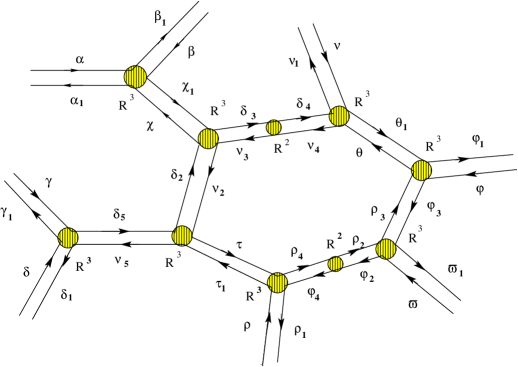
Figure 6: Example of network.

But the definition of the two- and three channel $R$-matrices given above doesn’t depend on the coordinates of the space; they are defined at the zero point. Therefore, in order to form a network with different positions of the scattering nodes, we should translate each of the scattering matrices from the zero point to their position at $\vec{\xi}$. This can be done by use of the set of translational matrices $W_{\vec{\xi}}(\vec{k_{i}})$, one for each of channels $(i=1,2,3)$, defined as

$$W_{\vec{\xi}}(\vec{k_{i}})=\left(\begin{array}[]{cc}1&0\\ 0&e^{i\vec{k_{i}}\vec{\xi}}\end{array}\right),\;i=1,3,\quad W_{\vec{\xi}}(\vec{k_{2}})=\left(\begin{array}[]{cc}e^{i\vec{k_{2}}\vec{\xi}}&0\\ 0&1\end{array}\right),$$ (3.84)

with $\vec{k_{i}}=k\vec{n_{i}}$, where $\vec{n_{i}}$ is unit vector exiting from the vertex $\vec{\xi}$ along a channel $i=1,2,3$ in direction to the neighbor vertex (defined by arrows on the figures). The matrices $W_{\vec{\xi}}(\vec{k_{i}})$ and $W_{\vec{\xi}}(\vec{k_{i}})^{-1}=W_{\vec{\xi}}(-\vec{k_{i}})$ are acting on the incoming and outgoing states of the channels respectively. On the matrix elements (3.2) of the $R$-matrix they act as:

$$R_{\alpha\beta\gamma}^{\alpha^{\prime}\beta^{\prime}\gamma^{\prime}}(\vec{\xi}) = (W_{\vec{\xi}}(\vec{k_{1}})^{-1})_{\alpha}^{\alpha_{1}}(W_{\vec{\xi}}(\vec{k_{1}}))_{\beta}^{\beta_{1}}(W_{\vec{\xi}}(\vec{k_{3}})^{-1})_{\gamma}^{\gamma_{1}}R_{\alpha_{1}\beta_{1}\gamma_{1}}^{\alpha_{2}\beta_{2}\gamma_{2}}$$ (3.85)

$$\cdot (W_{\vec{\xi}}(\vec{k_{2}}))_{\alpha_{2}}^{\alpha^{\prime}}(W_{\vec{\xi}}^{-1})(\vec{k_{2}}))_{\beta_{2}}^{\beta^{\prime}}(W_{\vec{\xi}}(\vec{k_{3}})))_{\gamma_{2}}^{\gamma^{\prime}}\quad$$

In the fermionic operator formulation (3.72), this transformation reads as

$$R_{123}(\vec{\xi})=(:e^{-(1-e^{-\vec{\xi}\vec{k_{1}}})c^{+}_{1}c_{1}}:)\;(:e^{(1-e^{\vec{\xi}\vec{k_{1}}})c^{+}_{2}c_{2}}:)\;(:e^{-(1-e^{-\vec{\xi}\vec{k_{3}}})c^{+}_{3}c_{3}}:)\;R_{123}$$

$$\times(:e^{-(1-e^{\vec{\xi}\vec{k_{2}}})c^{+}_{1}c_{1}}:)\;(:e^{(1-e^{-\vec{\xi}\vec{k_{2}}})c^{+}_{2}c_{2}}:)\;(:e^{-(1-e^{\vec{\xi}\vec{k_{3}}})c^{+}_{3}c_{3}}:),\qquad$$ (3.86)

which is equivalent to the corresponding change of the parameters $r_{ij}$ in (3.2). Namely,

$$r_{ij}(\vec{\xi})=e^{-(\vec{k}_{i}-\vec{k}_{j})\vec{\xi}}r_{ij},$$ (3.87)

where the $r_{ij}$ are defined in (3.57), (3.77).

The equation (3.87) gives also the transformation formula for the two-channel matrix elements of two-channel ${R^{(2)}}_{\alpha\beta}^{\alpha^{\prime}\beta^{\prime}}$.

With the notations of $R^{(3)}$-matrix elements (3.2), the resulting ${R^{(8)}}$-matrix elements, describing the process of Fig.6, can be written as

$${R^{(8)}}_{\gamma\;\gamma_{1}\;\delta\;\varpi_{1}\;\beta\;\beta_{1}\;\varphi\;\varphi_{1}}^{\alpha_{1}\;\alpha\;\delta_{1}\;\varpi\;\nu_{1}\;\nu\;\rho_{1}\;\rho}=\frac{1}{N}\sum(-1)^{p_{\tau_{1}}+p_{\chi}+p_{\theta}}$$

$${R^{(3)}}_{\gamma\gamma_{1}\delta}^{\delta_{5}\nu_{5}\delta_{1}}{R^{(3)}}_{\delta_{5}\nu_{5}\tau_{1}}^{\delta_{2}\nu_{2}\tau}{R^{(3)}}_{\chi\delta_{2}\nu_{2}}^{\chi_{1}\delta_{3}\nu_{3}}{R^{(3)}}_{\chi_{1}\beta\beta_{1}}^{\chi\alpha_{1}\alpha}{R^{(2)}}_{\delta_{3}\nu_{3}}^{\delta_{4}\nu_{4}}$$ (3.88)

$${R^{(3)}}_{\delta_{4}\nu_{4}\theta}^{\nu_{1}\nu\theta_{1}}{R^{(3)}}_{\varphi\varphi_{1}\theta_{1}}^{\varphi_{3}\rho_{3}\theta}{R^{(3)}}_{\varpi_{1}\varphi_{3}\rho_{3}}^{\varpi\varphi_{2}\rho_{2}}{R^{(2)}}_{\varphi_{2}\rho_{2}}^{\varphi_{4}\rho_{4}}{R^{(3)}}_{\varphi_{4}\rho_{4}\tau}^{\rho_{1}\rho\tau_{1}}$$

where we have summation over all internal repeating indexes.

The normalization factor $N$ in the expression (3.3) is essential to factor out vacuum(closed loop) processes in the network, which are going on without inclusion of external states. This factor will be concretely specified in examples presented in the next two sections. The signs $(-1)^{p}$ are reflecting the graded character of the $R$-operators (3.79): for recovering the formula (3.3), one has to make the product of the operators (3.79) corresponding to each vertex and to sum up over all the internal states.

One must also takes into account the following multiplication rules: if the product of two operators relative to a given internal channel $n$ contains a product such as ${}_{n}\langle\alpha|\times|\bar{\alpha}\rangle_{n}$, it must be evaluated using ${}_{n}\langle\alpha|\bar{\alpha}\rangle_{n}=\delta_{\alpha\bar{\alpha}}$, and if a product like $|\beta\rangle_{n}\times{}_{n}\langle\bar{\beta}|$ occurs, then it can be derived using: $|\beta\rangle_{n}\langle\bar{\beta}|=(-1)^{p_{\beta}}\delta_{\beta\bar{\beta}}$. This second relation can be obtained formally from $|\beta\rangle_{n}\langle\bar{\beta}|=(-1)^{p_{\beta}}{}_{n}\langle\bar{\beta}|\beta\rangle_{n}$, or exactly by introducing a supertrace over the states in the $n$-th channel.

It is clear that this procedure to express the total $R$-matrix via its constituents can be generalized to any complicated network. Below we are going to apply this technique to the bubble and triangle diagrams.

3.4 Action Formulation of the Networks

In this section we formulate the network problem in terms of the integral kernels of the $R$-operators (formulas 2.54,3.77) in the space of the Grassmanian functions and express an action principle for it.

As in subsection $3.2$, we attach to each local vertex with $m$-channels a fermionic vertex-function:

$$R_{m}(\{\bar{\psi}_{i},\psi_{j}\})=e^{-\sum^{m}r_{ij}\bar{\psi}_{i}\psi_{j}},$$ (3.89)

which is the kernel of the corresponding $R$-operator (3.79), the $r_{ij}$ being the entries of the $r$matrix describing the scattering process over that vertex. In order to find the $r-$matrix($S-$matrix) corresponding to the entire network, one must take the product of the $R$-operators (2.54,3.77) corresponding to the vertexes and integrate in the functional space over the internal fermionic fields.

Suppose that we have a network with $n$ vertices, each of which with $s_{i},\;i=1,\dots n$ internal links (which connect two vertices of the network) and $q_{i}$ external links (which are ending or starting in one vertex). Any link in the diagrams has its double with an opposite direction for the arrow). Let us denote the Grassmann-variables connected with the links of the $k$-th vertex as $\bar{\psi}^{k}_{i},\;\psi^{k}_{j}$: by a convention the variables $\bar{\psi}^{k}_{i}$ will be attached to the links with outgoing arrows, while the variables $\psi^{k}_{j}$ attached to the links with incoming arrows. Every internal link connects two vertices possessing two pairs of the Grassmann-variables: in the diagram below (Fig.7) they are $\bar{\psi}^{k}_{i},\;\psi^{k}_{i}$ and $\bar{\psi}^{k^{\prime}}_{i^{\prime}},\;\psi^{k^{\prime}}_{i^{\prime}}$.

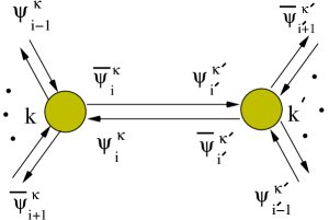
Figure 7: Attaching of the Grassmann-variables to the network.

Note that we are considering general networks, i.e.without any restriction on their structures, and, therefore, any two vertices can be connected by an arbitrary number of links. Below we denote the set of Fermi-fields on the internal links by $\mathcal{U}_{in}$, and the set of Fermi-fields on the external links by $\mathcal{U}_{ex}$.

Taking into account the integration rule for the product of integral kernels (2.53), the vertex-function associated to the network will be:

$${\cal R}(\{\bar{\psi}^{p}_{i},{\psi}^{p^{\prime}}_{i^{\prime}}\}\in{\mathcal{U}_{ex}})=e^{-\sum_{pp^{\prime}}\sum_{i,i^{\prime}\in{\mathcal{U}_{ex}}}\bar{\psi}^{p}_{i}{\bar{S}}^{pp^{\prime}}_{ii^{\prime}}\psi^{p^{\prime}}_{i^{\prime}}}=$$

$$= \frac{1}{N}\int\prod_{\{i,i^{\prime}\}\in{\mathcal{U}_{in}}}^{{}^{\prime}}\prod_{k,k^{\prime}}^{n}d\bar{\psi}^{k}_{i}d\psi^{k^{\prime}}_{i^{\prime}}\prod_{k}^{n}R_{k}(\{\bar{\psi}^{k}_{i},\psi^{k}_{i^{\prime}}\})$$

$$= \frac{1}{N}\int\prod_{\{i,i^{\prime}\}\in{\;\mathcal{U}_{in}}}^{{}^{\prime}}\prod_{k,k^{\prime}}^{n}\{d\bar{\psi}^{k}_{i}d\psi^{k^{\prime}}_{i^{\prime}}\;e^{-\bar{\psi}^{k}_{i}\psi^{k^{\prime}}_{i^{\prime}}}\}e^{-\sum_{i,j\in\mathcal{U}_{ex}\oplus\mathcal{U}_{in}}\sum_{k=1}^{n}r^{(k)}_{ij}\bar{\psi}^{k}_{i}\psi^{k}_{j}}.$$

Here $\mathcal{U}_{in}$ denotes also the set of internal links between the vertices with $dim[\mathcal{U}_{in}]=\sum_{j}^{n}s_{j}=2s$, where $s$ is the total number of the internal links in the network. Similarly $\mathcal{U}_{ex}$ is the set of external links and has dimension $q={{\sum_{k}^{n}q_{k}}}$, that is the number of the external links of the network. The indices $k,i$ and $k^{\prime},i^{\prime}$ in the measure of integration $e^{-\bar{\psi}^{k}_{i}\psi^{k^{\prime}}_{i^{\prime}}}$ correspond to the end points of the same link in the network (hence the mark ^′ appearing on the symbols in the products of (3.4) and in the sums of (3.91) below). The normalization factor $N$ is present in order for the mega-network $R$-matrix to appear in an exponential form (3.89) with an identity pre-factor. It is defined by the contribution of the closed loops to the functional integral (3.4).

The argument of the exponential function in the integrant in (3.4):

$${\cal A}(\{\bar{\psi}_{i}^{k},\psi_{i^{\prime}}^{k^{\prime}}\}\in\mathcal{U}_{in}\oplus\mathcal{U}_{ex})=-\sum_{i,i^{\prime}\in\mathcal{U}_{in}}^{{}^{\prime}}\sum_{k,k^{\prime}=1}^{n}\bar{\psi}^{k}_{i}\psi^{k^{\prime}}_{i^{\prime}}-\sum_{i,j\in\mathcal{U}_{ex}\oplus\mathcal{U}_{in}}\sum_{k=1}^{n}r^{(k)}_{ij}\bar{\psi}^{k}_{i}\psi^{k}_{j}$$ (3.91)

can be regarded as an action, and the normalization factor $N$ as a partition function for the corresponding network model with fixed external (boundary) fields. This interpretation allows also to calculate the $S$-matrix elements of the total network as a Green function of the external Fermi-fields:

$$(\mathcal{G})_{jj^{\prime}}^{pp^{\prime}}=({\bar{S}}^{-1})_{jj^{\prime}}^{pp^{\prime}}$$ (3.92)

$$=\frac{1}{NDet[\bar{S}]}\int\psi^{p^{\prime}}_{j^{\prime}}\bar{\psi}^{p}_{j}\prod_{\{i,i^{\prime}\}\in{\mathcal{U}_{in}\oplus\mathcal{U}_{ex}}}\prod_{k,k^{\prime}}^{n}d\bar{\psi}^{k}_{i}d\psi^{k^{\prime}}_{i^{\prime}}e^{-{\cal A}(\{\bar{\psi}_{i}^{k},\psi_{i^{\prime}}^{k^{\prime}}\}\in\mathcal{U}_{in}\oplus\mathcal{U}_{ex})}.$$

Now we will show that presented rules of calculation of the $S$-matrix of the mega network reproduces the star-product rules formulated in the articles [7]. A general proof of equivalence of two ways of calculations is available in a paper [16]. Here we will demonstrate their equivalence for so called bubble and triangle diagrams. Moreover, we show that the same result can be obtained via direct R-matrix products by following the rules presented in the example (3.3).

Let us separate the summands in the exponent which contain variables with internal indexes and represent the integral (3.4) in this way:

$$\frac{1}{N}e^{-\sum_{i,j\in{\mathcal{U}_{ex}}}\sum_{k}^{n}r^{(k)}_{ij}\bar{\psi}^{k}_{i}\psi^{k}_{j}}\int\prod_{\{i,i^{\prime}\}\in{\mathcal{U}_{in}}}\prod_{k,k^{\prime}}^{n}d\bar{\psi}^{k}_{i}d\psi^{k^{\prime}}_{i^{\prime}}\;$$ (3.93)

$$\cdot e^{-\sum_{i,j\in{\mathcal{U}_{ex}}}\sum_{i^{\prime},j^{\prime}\in{\mathcal{U}_{in}}}\sum_{k,k^{\prime}}^{n}\left(\bar{\psi}^{k}_{i^{\prime}}{A_{r}}_{i^{\prime}_{k}j^{\prime}_{k^{\prime}}}\psi^{k^{\prime}}_{j^{\prime}}+\bar{\psi}^{k}_{i}r^{(k)}_{ii^{\prime}}{\psi}^{k}_{i^{\prime}}+\bar{\psi}^{k^{\prime}}_{j^{\prime}}r^{(k^{\prime})}_{j^{\prime}j}\psi^{k^{\prime}}_{j}\right)}.$$

where $A_{r}$ is a $2s\times 2s$ matrix, with the elements ${A_{r}}_{i_{k}j_{k^{\prime}}}=\delta_{i_{k}j_{k^{\prime}}}+\delta_{kk^{\prime}}r^{(k)}_{ij}$, where in the second summand only the elements relative to the internal links are taken into account. This matrix, which contains only unit elements on the diagonal, can be presented in a block form after some rearrangement of the rows and columns , with $n$ diagonal blocks containing the parts of the $r^{(k)}$ matrices, referred to the internal links of the network, and $2s$ unity elements disposed out of the diagonal blocks in such a way that each column and each row contain only one unity element. When ”tadpole”-vertices are present in the networks, elements of the corresponding $r^{(k)}$ matrices also appear in the diagonal together with the unity elements.

After integration over internal $\psi^{\prime}s$ in the Gaussian integral (3.93), we arrive at:

$$e^{-\sum_{p,p^{\prime};i,i^{\prime}\in{\mathcal{U}_{ex}}}\bar{\psi}^{p}_{i}{\bar{S}}^{pp^{\prime}}_{ii^{\prime}}\psi^{p^{\prime}}_{i^{\prime}}}=\frac{\det{A_{r}}}{N}e^{-\sum_{i,j\in{\mathcal{U}_{ex}}}\left(\sum_{k}r^{(k)}_{ij}\bar{\psi}^{k}_{i}\psi^{k}_{j}-\sum_{k^{\prime},k^{\prime\prime}}A^{\;\;k^{\prime}k^{\prime\prime}}_{r\;ij}\bar{\psi}^{k^{\prime}}_{i}{\psi}^{k^{\prime\prime}}_{j}\right)},$$ (3.94)

from which it follows that the normalization factor $N$ in (3.4) must be equal to $\det{A_{r}}$ and the mega-$S$-matrix is:

$${\bar{S}}^{kk^{\prime}}_{ij}=r^{(k)}_{ij}\delta^{kk^{\prime}}-A^{\;\;kk^{\prime}}_{r\;ij},$$ (3.95)

where

$${A}^{\;\;kk^{\prime}}_{r\;ij}=\sum_{i^{\prime},j^{\prime}\in{\mathcal{U}_{in}}}^{2s}r^{(k)}_{ii^{\prime}}{(A_{r})}^{-1}_{i^{\prime}_{k}j^{\prime}_{k^{\prime}}}r^{(k^{\prime})}_{j^{\prime}j}$$ (3.96)

and $k,k^{\prime}$ are relative only to vertices which possess external legs.

Expression (3.94) easily follows after using Hubbard-Stratanovich transformation in (3.93) and:

$$\sum_{i^{\prime},j^{\prime}\in{\mathcal{U}_{in}}}^{2s}\left(\sum_{i\in{\mathcal{U}_{ex}}}^{q}\sum_{k}^{n}\bar{\psi}^{k}_{i}r^{(k)}_{ii^{\prime}}\right){(A_{r})}^{-1}_{i^{\prime}_{k}j^{\prime}_{k^{\prime}}}\left(\sum_{j\in{\mathcal{U}_{ex}}}^{q}\sum_{k^{\prime}}^{n}r^{(k^{\prime})}_{j^{\prime}j}\psi^{k^{\prime}}_{j}\right)=$$ (3.97)

$$= \sum_{i,j\in{\mathcal{U}_{ex}}}^{q}\sum_{k,k^{\prime}}^{n}A^{\;\;kk^{\prime}}_{r\;ij}\bar{\psi}^{k}_{i}{\psi}^{k^{\prime}}_{j}.$$

For the particular case $n=2$ let us write down a detailed expression of the network vertex-function (or the kernel of the $R$-operator corresponding to that network). Now the network contains two vertices having respectively $s_{1},\;q_{1}$ and $s_{2},\;q_{2}$ internal and external links. After dividing each of the $r^{(k)}$ matrices into four blocks, following the definitions in the work [7], the kernel function of $k$-th vertex can be represented as:

$$e^{-\sum_{i,j}^{s_{k}+q_{k}}r^{(k)}_{ij}\bar{\psi}^{k}_{i}\psi^{k}_{j}}=e^{-\sum_{i,j}^{2}{\mathrm{r}}^{(k)}_{ij}\bar{\Psi}^{k}_{i}\Psi^{k}_{j}}$$

Here $\Psi^{k}_{1}=\{\psi^{k}_{1},\cdots,\psi^{k}_{s_{k}}\}^{\tau}$ is the set of variables connected with the internal links of the $k$-th vertex, and $\Psi^{k}_{2}=\{\psi^{k}_{s_{k}+1},\cdots,\psi^{k}_{s_{k}+q_{k}}\}^{\tau}$ the set of variables connected with the external links. Correspondingly: $\bar{\Psi}^{k}_{1}=\{\bar{\psi}^{k}_{1},\cdots,\bar{\psi}^{k}_{s_{k}}\}$, $\bar{\Psi}^{k}_{2}=\{\bar{\psi}^{k}_{s_{k}+1},\cdots,\bar{\psi}^{k}_{s_{k}+q_{k}}\}$. It follows that: $r^{(k)}=\left(\begin{array}[]{cc}{\mathrm{r}}^{(k)}_{11}&{\mathrm{r}}^{(k)}_{12}\\ {\mathrm{r}}^{(k)}_{21}&{\mathrm{r}}^{(k)}_{22}\end{array}\right)$.

Now the expression (3.4) takes a simple form (it is obvious that $s_{1}=s_{2}=s$):

$$\displaystyle\int d\bar{\Psi}^{1}_{1}d\Psi^{2}_{1}d\bar{\Psi}^{2}_{1}d\Psi^{1}_{1}\exp\bigg{\{}-\bar{\Psi}^{1}_{1}\Psi^{2}_{1}-\bar{\Psi}^{2}_{1}\Psi^{1}_{1}-\sum_{k=1}^{2}\sum_{i,j}^{2}\bar{\Psi}^{k}_{i}{\mathrm{r}}^{(k)}_{ij}\Psi^{k}_{j}\bigg{\}}=$$

$$N\exp\Bigg{\{}\displaystyle-\sum_{k=1}^{2}{\mathrm{r}}^{(k)}_{22}\bar{\Psi}^{k}_{2}\Psi^{k}_{2}+\left(\bar{\Psi}^{2}_{2}{\mathrm{r}}^{(2)}_{21},\bar{\Psi}^{1}_{2}{\mathrm{r}}^{(1)}_{21}\right)A_{r}^{-1}{\left(\!\!\begin{array}[]{c}{\mathrm{r}}^{(1)}_{12}\Psi^{1}_{2}\\ {\mathrm{r}}^{(2)}_{12}\Psi^{2}_{2}\end{array}\!\!\!\right)}\Bigg{\}},$$ (3.100)

where

$$A_{r}=\left(\begin{array}[]{cc}\mathrm{I}&{\mathrm{r}}^{(1)}_{11}\\ {\mathrm{r}}^{(2)}_{11}&\mathrm{I}\end{array}\right),\qquad N=\det{A_{r}}=\det{(\mathrm{I}-{\mathrm{r}}^{(1)}_{11}{\mathrm{r}}^{(2)}_{11})}.$$ (3.103)

where $\mathrm{I}$ is the $s\times s$ unit matrix.

The quadratic function in (3.100) can be represent in a compact form as:

$$e^{-\sum_{i,j}^{2}\mathrm{r}^{(12)}_{ij}\bar{\Psi^{i}_{2}}\Psi^{j}_{2}},$$ (3.104)

with the $(q_{1}+q_{2})\times(q_{1}+q_{2})$ matrix $\mathrm{r}^{(12)}$:

$$\mathrm{r}^{(12)}=\left(\begin{array}[]{cc}\mathrm{r}^{(1)}_{22}-\mathrm{r}^{(1)}_{21}{[A_{r}^{-1}]}_{21}\mathrm{r}^{(1)}_{12}&-\mathrm{r}^{(1)}_{21}{[A_{r}^{-1}]}_{22}\mathrm{r}^{(2)}_{12}\\ &\\ -\mathrm{r}^{(2)}_{21}{[A_{r}^{-1}]}_{11}\mathrm{r}^{(1)}_{12}&\mathrm{r}^{(2)}_{22}-\mathrm{r}^{(2)}_{21}{[A_{r}^{-1}]}_{12}\mathrm{r}^{(2)}_{12}\end{array}\right),$$ (3.108)

and the inverse matrix $A_{r}^{-1}$ having a following form

$$A_{r}^{-1}=\left(\begin{array}[]{cc}[A_{r}^{-1}]_{11}&{[A_{r}^{-1}]}_{12}\\ &\\ {[A_{r}^{-1}]}_{21}&{[A_{r}^{-1}]}_{22}\end{array}\right)=\left(\begin{array}[]{cc}\left(\mathrm{I}-{\mathrm{r}}^{(1)}_{11}{\mathrm{r}}^{(2)}_{11}\right)^{-1}&-{\mathrm{r}}^{(1)}_{11}\left(\mathrm{I}-{\mathrm{r}}^{(2)}_{11}{\mathrm{r}}^{(1)}_{11}\right)^{-1}\\ &\\ -{\mathrm{r}}^{(2)}_{11}\left(\mathrm{I}-{\mathrm{r}}^{(1)}_{11}{\mathrm{r}}^{(2)}_{11}\right)^{-1}&\left(\mathrm{I}-{\mathrm{r}}^{(2)}_{11}{\mathrm{r}}^{(1)}_{11}\right)^{-1}\end{array}\right).$$ (3.109)

The results in (3.108) reproduce for the considered situation the rules of the generalized star-product, derived in [7]. The matrix $\mathrm{r}^{(12)}_{ij}$ describes the entire scattering process over the $2-$vertex network.

Now, let us note that the replacement of the local $r^{(k)}$-matrices by their unitary counterparts is equivalent to the unitary transformation of the mega $\bar{S}$-matrix. Here we are giving the proof of that statement. We introduce formal notation $\bar{\Psi}_{\mathcal{E}}S(r^{(k)})\Psi_{\mathcal{E}}=\sum_{p,p^{\prime};i,i^{\prime}\in{\mathcal{U}_{ex}}}\bar{\psi}^{p}_{i}{\bar{S}}^{pp^{\prime}}_{ii^{\prime}}\psi^{p^{\prime}}_{i^{\prime}}$, denoting by $\bar{\Psi}_{\mathcal{E}},\;{\Psi}_{\mathcal{E}}$ ($\bar{\Psi}_{\mathcal{I}},\;{\Psi}_{\mathcal{I}}$) the fermionic variables connected with the external (internal) links and by ${S}(r^{(k)})$ the global scattering matrix. We shall denote the action in (3.91)by $A(r^{(k)};\bar{\Psi}_{\mathcal{E}},{\Psi}_{\mathcal{E}},\bar{\Psi}_{\mathcal{I}},{\Psi}_{\mathcal{I}})$.

Then, performing a simple transformation of the Grassman variables

$$N(r^{(k)})e^{-\bar{\Psi}_{\mathcal{E}}S(r^{(k)})\Psi_{\mathcal{E}}}=\int D\bar{\Psi}_{\mathcal{I}}D\Psi_{\mathcal{I}}e^{-A(r^{(k)};\bar{\Psi}_{\mathcal{E}},{\Psi}_{\mathcal{E}},\bar{\Psi}_{\mathcal{I}},{\Psi}_{\mathcal{I}})}=$$ (3.110)

$$\int D\bar{\chi}_{\mathcal{I}}D\chi_{\mathcal{I}}e^{-A({r^{(k)}}^{\tau};\bar{\chi}_{\mathcal{I}},\chi_{\mathcal{I}},\bar{\chi}_{\mathcal{E}}\chi_{\mathcal{E}})}=N({r^{(k)}}^{\tau})e^{-\bar{\chi}_{\mathcal{E}}S({r^{(k)}}^{\tau})\chi_{\mathcal{E}}},$$

$${\textrm{where}}\quad{r^{(k)}}^{\tau}_{ij}={r^{(k)}}_{ji},\qquad\bar{\chi}=-{\Psi},\quad\chi=\bar{\Psi},$$ (3.111)

we are coming to the relations: $N({r^{(k)}}^{\tau})=N(r^{(k)})$ and $S({r^{(k)}}^{\tau})=S(r^{(k)})^{\tau}$. The following relation takes also place: $S({r^{(k)}}^{*})=S({r^{(k)}})^{*}$ where $*$ denotes complex conjugation.

If ${r^{(k)}}^{\dagger}={r^{(k)}}^{-1}$, then $S({r^{(k)}}^{-1})=S({r^{(k)}}^{*\tau})=S({r^{(k)}})^{*\tau}$. As $S(r^{(k)})$ is unitary, if $r^{(k)}$ is unitary matrix for each vertex $k$ (see [16]), then

$$S({r^{(k)}}^{-1})=S({r^{(k)}})^{-1}.$$ (3.112)

and $N({r^{(k)}}^{-1})=N(r^{(k)})^{*}$.

4 Bubble Diagram

Let us apply the technique developed above to the calculation of the bubble network-diagram presented in Fig.7. According to the prescription presented in the previous section the corresponding two particle $R$-matrix is:

$${R^{(}2)}_{\alpha\beta}^{\alpha_{2}\beta_{2}}=\frac{1}{N}\sum(-1)^{p_{\gamma}}{R^{(3)}}_{\alpha\;\;\beta\;\gamma}^{\alpha_{1}\beta_{1}\gamma_{1}}{R^{(3)}}_{\alpha_{1}\;\beta_{1}\;\gamma_{1}}^{\alpha_{2}\beta_{2}\gamma},$$ (4.113)

where $N$ is defined from ${R^{(2)}}_{01}^{01}=1$, as it follows from the expression of two particle R-matrix (2.17). This gives

$$N=\sum(-1)^{p_{\gamma}}{R^{(3)}}_{0\;1\;\gamma}^{\alpha_{1}\beta_{1}\gamma_{1}}{R^{(3)}}_{\alpha_{1}\beta_{1}\gamma_{1}}^{0\;1\;\gamma}.$$ (4.114)

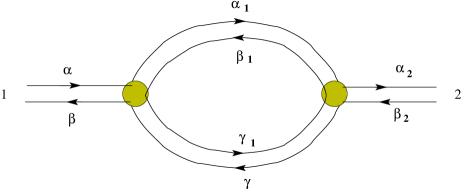
Figure 8: Bubble diagram constructed from two three channel vertices.

The calculations can be easily done with the Mathematica program. In order not to overload the text with heavy expressions, we will only present hereafter the result for scale invariant R-matrices as defined in [6], [11], [12]. We begin by stating the result which is particularly simple, namely:

Two scale invariant $R^{(3)}$-matrices with scaling parameters $\varrho_{1}$ and $\varrho_{2}$ respectively, are defining, via the expression (4.113), a scale invariant $R^{(2)}$ matrix with scaling parameter $\varrho_{1}\varrho_{2}$.

More explicitly, according to papers [6, 11, 12] and relation (3.57), a scale invariant S-matrix defines the following parameterisation for the R-matrix:

$$r_{11} = -\frac{\varrho}{a},\;\;r_{12}=\frac{1+\varrho}{a},\;\;r_{13}=\frac{(1+\varrho)\varrho}{a},$$

$$r_{21} = \frac{(1+\varrho)\varrho}{a},\;\;r_{22}=-\frac{\varrho}{a},\;\;r_{23}=\frac{1+\varrho}{a},$$

$$r_{31} = \frac{1+\varrho}{a},\;\;r_{32}=\frac{(1+\varrho)\varrho}{a},\;\;r_{33}=-\frac{\varrho}{a},$$

$$a = 1+\varrho+\varrho^{2}$$ (4.115)

Substituting expressions (4) into (4.113) and after renormalization of the product of the two $R^{(3)}$-matrices by N one will obtain:

$$r_{11}^{(2)} = \frac{2\varrho_{1}\varrho_{2}}{1+\varrho_{1}^{2}\varrho_{2}^{2}},\qquad r_{12}^{(2)}=\frac{1-\varrho_{1}^{2}\varrho_{2}^{2}}{1+\varrho_{1}^{2}\varrho_{2}^{2}}$$

$$r_{21}^{(2)} = \frac{-1+\varrho_{1}^{2}\varrho_{2}^{2}}{1+\varrho_{1}^{2}},\qquad r_{22}^{(2)}=\frac{2\varrho_{1}\varrho_{2}}{1+\varrho_{1}^{2}\varrho_{2}^{2}},$$ (4.116)

which is precisely the parameterisation of the scale invariant two particle S-matrix with scaling parameter $\varrho_{1}\varrho_{2}$ defined in [6, 11, 12]!

The bubble diagram we are considering is obviously the simplest non-trivial $2$-vertex loop diagram. The $2\times 2$ matrix $r_{ij}$ can be constructed directly by use of both (3.108) and (4.113) formulas. Let us denote by $r_{ij}^{(k)}$ ($k=1,\;2$) the two $3\times 3$ matrices, each corresponding to one vertex. The numeration is taken so that the second channel of the first vertex (internal links) corresponds to the first channel of the second vertex, and the third channel of the first vertex is connected with the third channel of the second vertex. The first channel of the first vertex and the second channel of the second vertex correspond to the external links. The $r_{ij}$ matrix of the final two channel process can be expressed by the following expression [7]:

$$r_{ij}=\left(\!\!\!\begin{array}[]{cc}r^{(1)}_{11}&0\\ 0&r^{(2)}_{22}\end{array}\!\!\!\right)+\left(\!\!\!\begin{array}[]{cccc}r^{(1)}_{12}&r^{(1)}_{13}&0&0\\ 0&0&r^{(2)}_{21}&r^{(2)}_{23}\end{array}\!\!\!\right)\left[A_{12}^{-1}\right]\left(\!\!\!\begin{array}[]{cc}r^{(2)}_{12}&0\\ r^{(2)}_{32}&0\\ 0&r^{(1)}_{21}\\ 0&r^{(1)}_{31}\end{array}\!\!\!\right),$$ (4.125)

where

$$A_{12}=\left(\!\!\!\begin{array}[]{cccc}1&0&r^{(1)}_{22}&r^{(1)}_{23}\\ 0&1&r^{(1)}_{32}&r^{(1)}_{33}\\ r^{(2)}_{11}&r^{(2)}_{13}&1&0\\ r^{(2)}_{31}&r^{(2)}_{33}&0&1\end{array}\!\!\!\right).$$ (4.130)

The normalization factor $N$ equals to

$$N = \mathrm{Det}[A_{12}]=\mathrm{Det}\left[\left(\!\!\!\begin{array}[]{cc}1&0\\ 0&1\end{array}\!\!\!\right)-\left(\!\!\!\begin{array}[]{cc}r^{(1)}_{22}&r^{(1)}_{23}\\ r^{(1)}_{32}&r^{(1)}_{33}\end{array}\!\!\!\right)\left(\!\!\!\begin{array}[]{cc}r^{(2)}_{11}&r^{(2)}_{13}\\ r^{(2)}_{31}&r^{(2)}_{33}\end{array}\!\!\!\right)\right]\qquad$$ (4.137)

$$= 1-r^{(1)}_{22}r^{(2)}_{11}-r^{(1)}_{33}r^{(2)}_{33}-r^{(1)}_{32}r^{(2)}_{13}-r^{(1)}_{23}r^{(2)}_{31}$$

$$+ \left(r^{(1)}_{22}r^{(1)}_{33}-r^{(1)}_{32}r^{(1)}_{23}\right)\left(r^{(2)}_{11}r^{(2)}_{33}-r^{(2)}_{13}r^{(2)}_{31}\right).$$

Note that the same expression (4.137) for $N$ can be obtained directly from formula (4.114) by use of Mathematica program.

5 Triangle Vertex

In the most general case, the three particle R-matrix is anisotropic and its elements depend on the channels 1,2,3. In such a case, it is necessary to specify, in the network diagrams, the channels of all the three particle vertices and follow which channels of neighboring vertices are connected. It is clear that all $3^{3}=27$ types of connections in the triangle are in general possible and this will be defined by the considered problem itself. Here, as an example, we will present the case corresponding of the disposition of vertices as depicted in Fig.8. Namely, the second channel of the first vertex is connected with the first channel of second vertex, the third channel of the second vertex is connected with the second channel of the third vertex and the first channel of third vertex is connected with the third channel of the first vertex. Notice that, according to Fig.5, the pairs of indexes ($\alpha,\beta$), ($\beta^{\prime},\alpha^{\prime}$) and ($\gamma,\gamma^{\prime}$) at the first, second and third position of ${R}$ are correspond to the first, second and third channel respectively.

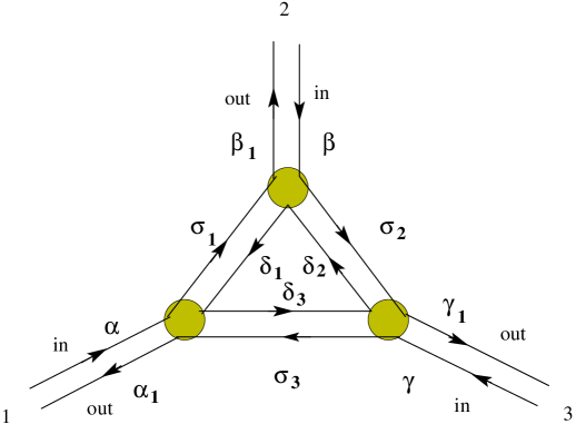
Figure 9: Triangle diagram constructed from three three-channel R-matrices.

Then, according to the prescription defined above, the ${R}$-matrix corresponding to triangle diagram reads as:

$${R^{(\Delta)}}_{\beta_{1}\alpha\alpha_{1}}^{\beta\gamma_{1}\gamma}=\frac{1}{N}\sum R_{\alpha\alpha_{1}\sigma_{3}}^{\sigma_{1}\delta_{1}\delta_{3}}R_{\beta_{1}\sigma_{1}\delta_{1}}^{\beta\sigma_{2}\delta_{2}}R_{\sigma_{2}\delta_{2}\delta_{3}}^{\gamma_{1}\gamma\sigma_{3}}(-1)^{p_{\sigma_{3}}}.$$ (5.139)

The normalization factor $N$ is defined by the condition

$${R^{(\Delta)}}_{101}^{101}=1.$$ (5.140)

The matrix $r^{(123)}_{ij},\;i,j=1,2,3$ describing the scattering over the triangle-graph in accordance with the formulas (3.72) and (3.94) is:

$$r^{(123)}=\left(\begin{array}[]{ccc}r^{(1)}_{11}&0&0\\ 0&r^{(2)}_{22}&0\\ 0&0&r^{(3)}_{33}\end{array}\right)+$$ (5.144)

$$+ \left(\begin{array}[]{cccccc}0&0&r^{(1)}_{12}&0&0&r^{(1)}_{13}\\ 0&r^{(2)}_{21}&0&0&r^{(2)}_{23}&0\\ r^{(3)}_{31}&0&0&r^{(3)}_{32}&0&0\end{array}\right)A_{123}^{-1}\left(\begin{array}[]{ccc}r^{(1)}_{31}&0&0\\ r^{(1)}_{21}&0&0\\ 0&r^{(2)}_{12}&0\\ 0&r^{(2)}_{32}&0\\ 0&0&r^{(3)}_{23}\\ 0&0&r^{(3)}_{13}\end{array}\right),$$ (5.154)

where $r_{ij}^{(k)},\;\;k=1,2,3$ are the R-matrix parameters in the three vertices of the triangle diagram on Fig.9. and

$$A_{123} = \left(\begin{array}[]{cccccc}1&0&r^{(1)}_{32}&0&0&r^{(1)}_{33}\\ 0&1&r^{(1)}_{22}&0&0&r^{(1)}_{23}\\ 0&r^{(2)}_{11}&1&0&r^{(2)}_{13}&0\\ 0&r^{(2)}_{31}&0&1&r^{(2)}_{33}&0\\ r^{(3)}_{21}&0&0&r^{(3)}_{22}&1&0\\ r^{(3)}_{11}&0&0&r^{(3)}_{12}&0&1\end{array}\right),$$ (5.161)

with

$$N=\det{A_{123}}.\qquad$$ (5.162)

Again, the calculations of ${{R}^{(\Delta)}}_{\beta_{1}\alpha\alpha_{1}}^{\beta\gamma_{1}\gamma}$ can be done with a simple Mathematica program. We will not present here the 20 big formulas, but just show the normalization factor $N$:

$$N = \sum R_{0\;1\;\sigma_{3}}^{\sigma_{1}\delta_{1}\delta_{3}}R_{1\;\sigma_{1}\delta_{1}}^{1\;\sigma_{2}\delta_{2}}R_{\sigma_{2}\delta_{2}\delta_{3}}^{0\;1\;\sigma_{3}}(-1)^{p(\sigma_{3})}$$

$$= \left(1-r^{(1)}_{22}r^{(2)}_{11}\right)\left(1-r^{(1)}_{33}r^{(3)}_{11}\right)\left(1-r^{(2)}_{33}r^{(3)}_{22}\right)$$

$$+ r^{(1)}_{23}r^{(2)}_{31}r^{(3)}_{12}+r^{(1)}_{32}r^{(2)}_{13}r^{(3)}_{21}-r^{(1)}_{33}r^{(2)}_{33}r^{(3)}_{12}r^{(3)}_{21}$$

$$- r^{(1)}_{22}r^{(2)}_{13}r^{(2)}_{32}r^{(3)}_{22}-r^{(1)}_{32}r^{(1)}_{23}r^{(2)}_{11}r^{(3)}_{11}+r^{(1)}_{22}r^{(1)}_{33}r^{(2)}_{11}r^{(2)}_{33}r^{(3)}_{11}r^{(3)}_{22}$$

$$- \left(r^{(1)}_{22}r^{(1)}_{33}-r^{(1)}_{23}r^{(1)}_{32}\right)\left(r^{(2)}_{11}r^{(2)}_{33}-r^{(2)}_{13}r^{(1)}_{31}\right)\left(r^{(3)}_{11}r^{(3)}_{22}-r^{(3)}_{12}r^{(3)}_{21}\right).$$

6 Conclusions

We have presented a new approach to the calculation of complicated mega-S-matrices of the arbitrary network based on two ways:

• Introducing R-matrices which are defined by the S-matrices of the local scatterings and taking the product of such R-matrices;

• Formulating an action for the corresponding network by use of fermionic fields.

In the examples of bubble and triangle diagrams we show the equivalence of this technique of computations with the generalized star-product procedure. The general proof valid in the case of an arbitrary graph was given in [16].

The action formulation has several advantages. First of all, it allows one to investigate network models with large number ($N\rightarrow\infty$) and random disposition of vertices and formulate corresponding quantum field theory, which will boost further investigations. In this language one can take also sum over random dispositions of scatterers and analyze the problem of Anderson localization. Secondly, the approach makes the calculation of mega-$S$-matrix elements of the regular,i.e. having some translational symmetry, networks very simple. Then the problem simply reduces to Fourier analysis of the action on a particular lattice defined by the network. This statement was demonstrated in Section 2 on a model of a chain of equidistant impurities. The third, and presumably most important advantage of the action formulation, is a possibility to generalize networks and consider models with multiparticle interactions.

7 Acknowledgments

We appreciate discussions with M.Karowski, M.Mintchev and R.Schrader. A.S. acknowledge LAPTH and University of Savoie for hospitality, where part of this work was done. P.S. is indebted to L.Alvarez-Gaumé and the CERN Theory Division for its stimulating and warm atmosphere.

References

- [1] ”Analysis on Graphs and its Applications” Proceedings of Symposia in Pure Mathematics, Vol.77 (2008), American Mathematical society, Exner et al. Editors.
- [2] C. Nayak, M. P. A. Fisher, A. W. W. Ludwig and H. H. Lin, Resonant multilead point-contact tunneling, Phys. Rev. B 59 (1999) 15 694–15 704.
- [3] X. Barnabe-Theriault, A. Sedeki, V. Meden, K. Schönhammer, Junctions of one-dimensional quantum wires: correlation effects in transport, Phys. Rev. B 71 (2005) 205327-1–13.
- [4] M. Oshikawa, C. Chamon and I. Affleck, Junctions of three quantum wires, J. Stat. Mech. 0602 (2006) P008 [arXiv:cond-mat/0509675].
- [5] S. Das, S. Rao and D. Sen, Interedge interactions and fixed points at a junction of a quantum Hall junction, Phys. Rev. B 74 (2006) 045322-1–5.
- [6] V. Kostrykin and R. Schrader, Kirchhoff’s rule for quantum wires, J. Phys. A 32 (1999) 595–630.
- [7] V. Kostrykin and R. Schrader, The Generalized Star Product and the Factorization of Scattering Matrices on Graphs, J. Math. Phys. 42 (2001) 1563 – 1598.
- [8] V. Kostrykin and R. Schrader, The inverse scattering problem for metric graphs and the traveling salesman problem, preprint arXiv:math-ph/0603010 (2006)
- [9] M. Mintchev, E. Ragoucy and P. Sorba, Reflection-transmission algebras, J. Phys. A 36 (2003) 10407–10429 [arXiv:hep-th/0303187].
- [10] B. Bellazzini and M. Mintchev, Quantum fields on star graphs, J. Phys. A 39 (2006) 11101–11117 [arXiv:hep-th/0605036].
- [11] B. Bellazzini, M. Mintchev and P. Sorba, Bosonization and scale invariance on quantum wires, J. Phys. A 40 (2007) 2485–2507 [arXiv:hep-th/0611090].
- [12] B. Bellazzini,M. Burrello, M. Mintchev and P. Sorba, Quantum field theory on Star Graphs, Proceedings of Symposia in Pure Mathematics, vol.77,2008,p.639 [arXiv:0801.2852[hep-th]].
- [13] M. Mintchev and E. Ragoucy, Algebraic approach to multiple defects on the line and application to Casimir force, J. Phys. A 40 (2007) 9515– [arXiv:0705.1322 [hep-th]].
- [14] E. Ragoucy, Quantum field theory on quantum graphs ans application to their conductance , LAPTH-1304/09 [arXiv:0901.2431[hep-th]].
- [15] A. Sedrakyan, Edge excitations of an incompressible fermionic liquid in a staggered magnetic field, Nucl.Phys.B 554 [FS] (1999) 514–536. [arXiv:cond-mat/9806301].
- [16] Sh. Khachatryan, R. Schrader, A. Sedrakyan, Grassmann–Gaussian integrals and generalized star products, Submitted to Journal. Phys. A: Math.Gen. [arXiv:math-ph/0904.2683].
- [17] J. Chalker, P. Coddington, J. Phys. C 21 2665 (1988).
- [18] A.Sedrakyan, On the theory of plateau plateau transitions in the quantum Hall effect Phys. Rev.B 68, 235329 (2003).[arXiv:cond-mat/0303349].
- [19] D.Arnaudon, R.Poghossian, A.Sedrakyan, P.Sorba, Integrable chain model with additional staggered model parameter, Nucl.Phys. B 588 [FS] (2000) 638–655. [arXiv:hep-th/0002123].
- [20] J.Ambjrn, Sh.Khachatryan, A.Sedrakyan, An integrable model with a non-reducible three particle R-matrix,J.Phys.A: Math.Gene. 37 (2004) 7397–7406.[arXiv:cond-mat/0403513].
- [21] M.Mintchev and P.Sorba, Finite temperature quantum field theory with impurities, JSTAT 0407 (2004) P001 [arXiv:hep-th/0405264]; Bosonisation and vertex algebras with defects, Annales Henri Poincare (2006) 1375-1393 [arXiv:hep-th/0511162].
- [22] J. Ambjrn, D.Karakhanyan, M. Mirumyan, A.Sedrakyan, Fermionization of the spin-S Uimin-Lai-Sutherland model: generalisation of the supersymmetric t-J model to spin-S, Nucl. Phys. B599 [FS] (2001) 547–560.
- [23] Y. Umeno, M. Shiroishi, M. Wadati, Fermionic R-operator for the Fermi chain model , hep- th/9806083; cond-mat/9806144.