Response of the solar atmosphere to magnetic field evolution
in a coronal hole region

Abstract

Context. Coronal holes (CHs) are deemed to be the sources of the fast solar wind streams that lead to recurrent geomagnetic storms and have been intensively investigated, but not all the properties of them are known well.

Aims. We mainly research the response of the solar atmosphere to the magnetic field evolution in a CH region, such as magnetic flux emergence and cancellation for both network (NT) and intranetwork (IN).

Methods. We study an equatorial CH observed simultaneously by HINODE and STEREO on July 27, 2007. The HINODE$/$SP maps are adopted to derive the physical parameters of the photosphere and to research the magnetic field evolution and distribution. The G band and Ca ii H images with high tempo-spatial resolution from HINODE$/$BFI and the multi-wavelength data from STEREO$/$EUVI are utilized to study the corresponding atmospheric response of different overlying layers.

Results. We explore an emerging dipole locating at the CH boundary. Mini-scale arch filaments (AFs) accompanying the emerging dipole were observed with the Ca ii H line. During the separation of the dipolar footpoints, three AFs appeared and expanded in turn. The first AF divided into two segments in its late stage, while the second and third AFs erupted in their late stages. The lifetimes of these three AFs are 4, 6, 10 minutes, and the two intervals between the three divisions or eruptions are 18 and 12 minutes, respectively. We display an example of mixed-polarity flux emergence of IN fields within the CH and present the corresponding chromospheric response. With the increase of the integrated magnetic flux, the brightness of the Ca ii H images exhibits an increasing trend. We also study magnetic flux cancellations of NT fields locating at the CH boundary and present the obvious chromospheric and coronal response. We notice that the brighter regions seen in the 171 Å images are relevant to the interacting magnetic elements. By examining the magnetic NT and IN elements and the response of different atmospheric layers, we obtain good positive linear correlations between the NT magnetic flux densities and the brightness of both G band (correlation coefficient 0.85) and Ca ii H (correlation coefficient 0.58).

1 Introduction

Coronal holes (CHs) are regions on the Sun where the magnetic fields are dominated by one magnetic polarity and the magnetic lines are open to interplanetary space (Bohlin 1977). These unipolar structures are presumed to originate at about 0.7 R_⊙ distance from the solar center (Stepanian 1995). CHs were identified as early as in 1951 by Waldmeier (1951) from the earliest photo of the solar corona. Observed with X-ray (Underwood & Muney 1967) and EUV line (Reeves & Parkinson 1970), they appear as dark and void areas due to their lower densities and lower temperatures compared with that of the quiet Sun (QS) (Munro & Withbroe 1972; Harvey 1996). But if observed with He i 10830 Å line, they are brighter areas (Zirker 1977; Harvey & Sheeley 1979). CHs are usually classified into three different categories according to their locations and lifetimes: polar, non-polar (isolated), and transient (Harvey & Recely 2002). Polar CHs can persist for about several years, non-polar ones always many solar rotations, while transient ones only several days. They are deemed to be the sources of the fast solar wind streams that lead to recurrent geomagnetic storms (Krieger et al. 1973; Tsurutani & Gonzalez 1987; Crooker & Cliver 1994; Cranmer 2002; Tu et al. 2005).

A mass of research concerning CHs has been extensively done in recent years. These studies refer nearly all the properties of CHs, such as positional distribution and periodic variation (Belenko 2001; Maravilla et al. 2001; Harvey & Recely 2002; Bilenko 2002, 2004; Hofer & Storini 2002; Mahajan et al. 2002; Temmer et al. 2007), magnetic field structure (Meunier 2005; Wiegelmann et al. 2005; Tian et al. 2008), magnetic field evolution (Wang & Sheeley 2004; Yamauchi et al. 2004; Zhang et al. 2006), temperature variation (Patsourakos et al. 2002; Wilhelm 2006; Zhang et al. 2007), element abundance (Feldman & Laming 2000; Laming & Feldman 2003), Doppler velocity (Raju et al. 2000; Stucki et al. 2000, 2002; Jordan et al. 2001; Wilhelm et al. 2002; Kobanov et al. 2003; Xia et al. 2003, 2004; Akinari 2007; Teplitskaya et al. 2007), fast solar wind (Giordano et al. 2000; Hackenberg et al. 2000; Patsourakos & Vial 2000; Wilhelm et al. 2000; Teriaca et al. 2003; Zhang et al. 2002, 2003, 2005a; Janse et al. 2007) and wave in CH (Moran 2003; Zhang 2003; Markovskii & Hollweg 2004; O’Shea et al. 2005, 2006, 2007; Zhang et al. 2005b; Dwivedi et al. 2006; Kobanov & Sklya 2007; Srivastava et al. 2007; Wu et al. 2007).

According to previous studies, CHs are not absolutely unipolar and there exist many closed coronal loops (eg. Levine 1977; Zhang et al. 2006). The magnetic network (NT; Leighton et al. 1962) elements are believed to be consisted of both low-lying loops and large-scale open magnetic funnels (Dowdy et al. 1986; Dowdy 1993), while the intranetwork (IN; Livingston & Harvey 1975) ones only contribute low-lying loops (Wiegelmann & Solanki 2004; Wiegelmann et al. 2005). In equatorial CHs, the chromosphere and transition region are highly structured. Their structures are similar to those in the QS region (Warren & Winebarger 2000; Feldman et al. 2001). Above the upper transition region, if observed with X-ray or EUV line, most of the structures disappear and the corona becomes much darker and more homogeneous than in the QS, except for some bright points (Xia et al. 2004).

Magnetic flux emergence and cancellation are the main forms of magnetic field evolution in the Sun (Zhang et al. 1998a$-$c). In an emerging flux region, new emerging dipoles may lead to the formation of arch filament systems (AFSs). AFSs were first studied by Bruzek (1967), whereafter their properties, such as size, shape, lifetime, evolution, structure and so on, have been extensively investigated (Bruzek 1969; Weart 1970; Frazier 1972; Chou & Zirin 1988; Alissandrakis et al. 1990; Georgakilas et al. 1990; Tsiropoula et al. 1992; Chou 1993). The reconnection occurring at CH boundaries is crucial to the evolution and rigid rotation of CHs (Wang et al. 1996; Kahler & Hudson 2002).

There is always a good correlation between the QS magnetic NT elements and the chromospheric structures since the magnetic NT features are always bright in the Ca ii line (Leighton 1959; Frazier 1970; Skumanich et al. 1975; Stenflo & Harvey 1985; Zirin 1988; Rezaei et al. 2007). Although the studies from Sivaraman & Livingston (1982) and Sivaraman et al. (2000) reveal that magnetic concentrations play a major role in the formation of Ca ii K line IN elements and there is a one-to-one relationship between K line IN bright elements and magnetic features, some other authors (eg. Remling et al. 1996; Steffens et al. 1996) report that there is no correlation between small-scale magnetic elements and locations of bright Ca K_2υ IN elements. Nindos & Zirin (1998) studied quantitatively the relation between the intensity of Ca ii K line bright features and the intensity of the associated magnetic elements in the QS. They found that there is an almost linear correlation between the K-line intensities and the absolute values of the magnetic field strength for the stronger NT elements, while this correlation disappears for the weaker magnetic elements. Lites et al. (1999) investigated the QS IN and found no direct correlation between the presence of magnetic features with apparent flux density above 3 Mx cm^-2 and the occurrence of H_2υ brightenings. They also found no correspondence between H_2υ grains and the horizontal-field IN features. Then Worden et al. (1999) found only a random correspondence between bright cell grains and regions of IN magnetic flux as seen in H i Ly$\alpha$ and 160 nm lines. Recently, Rezaei et al. (2007) investigated the relationship between the photospheric magnetic field and the emission of the mid-chromosphere and found that the emission in the NT is correlated with the magnetic flux density while there is no correlation between the integrated emission of Ca core-line and the magnetic flux density in the IN.

Owing to the restriction of observations, not all the characteristics of CHs are known well. Several newly launched space-based instruments, especially HINODE (Kosugi et al. 2007), have provided unprecedentedly high spatial and temporal resolution data, which is just the extremely important factor of investigating the fine structures in detail. Furthermore, multi-passband images from the Solar Terrestrial Relations Observatory (STEREO; Howard et al. 2008; Kaiser et al. 2008) give us plentiful information about the solar atmosphere. These data can be used together to study the magnetic field evolution and the response of overlying atmosphere, which will be helpful for us to understand the physical mechanism of the coronal heating and the solar wind acceleration.

In order to study magnetic flux emergence, cancellation, distribution, and the atmospheric response of different overlying layers in CHs, we investigate an equatorial CH of predominantly negative polarity in this paper. In Sect. 2, we introduce the observations and data analysis. In Sect. 3, we give some typical examples of small-scale magnetic field evolution and the corresponding atmospheric response, as well as the relationship between the magnetic intensities and the brightness of overlying solar atmosphere. The conclusions and discussion are presented in Sect. 4.

2 Observations and data analysis

Table 1: Data sets mainly used in this study.

Data Set	Observation	Cadence	Pixel Size	FOV
		(minutes)	(arcsec)	(arcsec2)
I	HINODE$/$SP	32a	0.32	151.14${\times}$162.30
II	HINODE$/$Gband	2	0.11	223.15${\times}$111.58
	HINODE$/$Ca ii H	2	0.11	223.15${\times}$111.58
III	STEREO$/$304	10	1.59	full disk
	STEREO$/$171	2.5	1.59	full disk
	STEREO$/$195	10	1.59	full disk
	STEREO$/$284	20	1.59	full disk

• Scan time for one SP map.

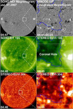
Figure 1: SOHO$/$MDI full-disk magnetogram (top left), SOHO$/$EIT 195 Å image (middle left), and STEREO$/$EUVI 304 Å image (bottom left). Three windows in the three full-disk images outline the FOV of HINODE$/$SP magnetograms. The right column shows a line-of-sight magnetogram from HINODE$/$SP, a 195 Å image and a 304 Å image from STEREO from top to bottom. The magnetograms from MDI and SP are displayed with (-50 G, 50 G) and (-80 G, 80 G) scales, respectively. The blue curves delineate the CH boundary derived from the STEREO$/$EUVI 284 Å image obtained at 04:46 UT, while the dotted lines indicate the FOV of the G band and Ca ii H images. The rectangles in the top-right image delineate the regions (“I”, “II”, “III”) that are specially studied.

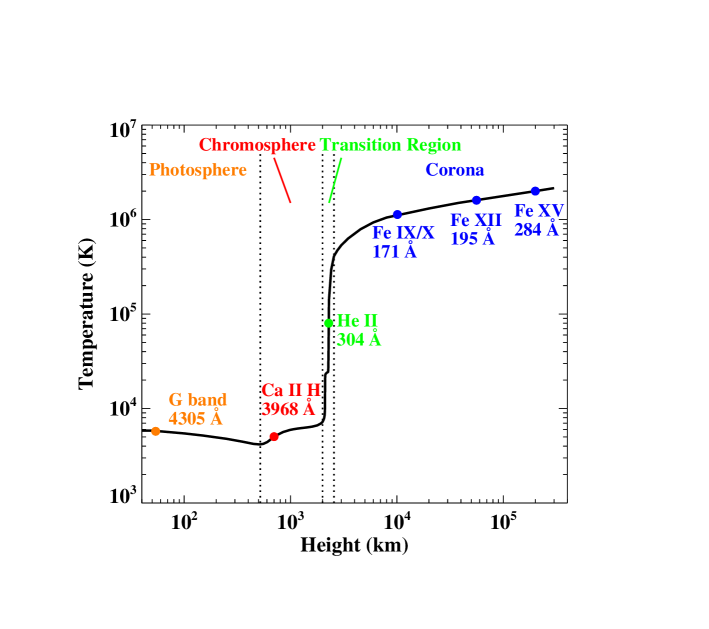
Figure 2: Variation of the temperature versus the height above the $\tau_{5000}$=1 (optical depth unity in the continuum at 5000 Å) surface. The G band and Ca ii H lines are emitted respectively in the lower photosphere and lower chromosphere, and their mean formation heights (54 km and 700 km, respectively) are all marked with filled circles in this figure. The peak formation temperatures of He ii (304 Å) line emitted in the transition region, and Fe ix$/$x (171 Å), Fe xii (195 Å), Fe xv (284 Å) lines which are all emitted in the inner solar corona are 80 000 K, 1.3 MK, 1.6 MK, 2.0 MK, respectively. They are also marked with filled circles in this figure.

The observations were carried out on July 27, 2007, using the Solar Optical Telescope (SOT; Ichimoto et al. 2008; Shimizu et al. 2008; Suematsu et al. 2008; Tsuneta et al. 2008) instrument on board HINODE, the Extreme Ultra Violet Imager (EUVI; Howard et al. 2008) telescope of the Sun-Earth Connection Coronal and Heliospheric Investigation (SECCHI; Howard et al. 2008) instrument aboard STEREO, the Michelson Doppler Imager (MDI; Scherrer et al.1995) and Extreme-ultraviolet Imaging Telescope (EIT; Delaboudinière et al. 1995) onboard the Solar and Heliospheric Observatory (SOHO; Domingo et al. 1995).

The data sets mainly used in this study are summarized in Table 1. The Spectro-Polarimeter (SP; Lites et al. 2001) in HINODE$/$SOT provides observations in four modes: normal, fast, dynamics and deep maps. Five sets of HINODE$/$SP maps adopted here were observed in fast map mode between 01:36 UT and 05:58 UT. They are all centered at about 11^∘W and 1^∘S and cover a large fraction of a CH area. Each map is constructed from 512${\times}$512 Stokes (I, Q, U and V) profiles of the photospheric Fe i 6301.5 Å and 6302.5 Å lines with a spectral sampling of 21.5 mÅ. The noise level in the continuum polarization is about 1.5$\times$10^-3 I_c. For the observation of each spectrograph slit, the integrated exposure time is 3.2 s. The scan direction is along the east-west direction with a scan step of 0″.295.

By using the Stokes spectrum inversion code based on the assumption of Milne-Eddington atmospheres (Yokoyama, T. private communication), we have successfully derived from the raw data numerous physical parameters, such as the three components of magnetic fields (the field strength B, the inclination angle $\gamma$, and the azimuth angle $\phi$), the stray light fraction $\alpha$, and the Doppler velocity V_los. Here, $\gamma$ is the angle between the vector magnetic field B and the LOS direction, and $\phi$ is the angle from the east$-$west direction to the projection of B on the plane perpendicular to the LOS direction. Then the vector magnetic field B is shown by the LOS field (1$-$$\alpha$)B$\cos$$\gamma$ and the transverse field (1$-$$\alpha$)^1/2B$\sin$$\gamma$. The Doppler shifts are derived from the Fe i 6302.5 Å Stokes I profiles and averaged over the whole field of view (FOV) of the SP maps.

Also employed from HINODE are G band and Ca ii H images obtained by the Broadband Filter Imager (BFI; Kosugi et al. 2007). Their FOV only covers part of the SP maps (shown with the dotted lines in Fig. 1). Moreover, we adopt the EUVI data from satellite A of STEREO. The EUVI telescope observed the full-Sun in four spectral channels (304 Å, 171 Å, 195 Å and 284 Å). The HINODE$/$BFI and STEREO$/$EUVI images used here are selected according to the scanning time of the SP maps.

The images are all prepared by applying the standard processing routines, including flat field correction, dark current and pedestal subtraction, bad camera pixel correction, camera readout error correction, cosmic ray removal, et al.. Then we co-align all the images and SP maps carefully. Since both G band and Ca ii H observations were taken with fixed pointing, first we co-align these images to each other. The bright features of Ca ii H line images are highly coincident with the underlying magnetic field features both in location and shape especially for NT elements (Warren & Winebarger 2000; Feldman et al. 2001; Xia et al. 2004), so we use the bright points to co-align the G band and Ca ii H images with the LOS magnetograms. For the co-alignment between the STEREO images and the SP maps, we look to the SOHO$/$MDI and SOHO$/$EIT images for help. At first, the LOS magnetograms (SP maps) from HINODE are co-aligned to the MDI full-disk magnetograms. Since the EIT and MDI images are from the same satellite and they can be co-aligned easily, so the SP maps can be co-aligned to the EIT images with no difficulty. Then the STEREO 195 Å images are co-aligned to the SOHO 195 Å images according to their bright features. After that, the STEREO 195 Å images (also 304 Å, 171 Å and 284 Å) have been co-aligned with the SP maps.

We determine the CH boundary with the brightness gradient method developed by Shen et al. (2006). In an EUV 284 Å image, each pixel has its own recorded brightness, b. For any given value of b, we can plot the contour and then calculate the area, A, enclosed by each contour. The derivation f=$\delta$b$/$$\delta$A is used to determine the boundary of a CH. The CH boundary is at the place where f=f_max.

Figure 1 shows a SOHO$/$MDI magnetogram (top left), a SOHO$/$EIT 195 Å image (middle left) and a STEREO$/$EUVI 304 Å image (bottom left). Three windows in the three full-disk images outline the FOV of HINODE$/$SP magnetograms. The right column shows respectively a LOS magnetogram from HINODE, a 195 Å image and a 304 Å image from STEREO. In order to improve the image contrast to visualize the fine structures better, a log-logarithmic scale is applied to the STEREO images presented in all the figures.

Figure 2 shows the typical variation of the temperature versus the height of the solar atmosphere above the $\tau_{5000}$=1 surface (Reeves et al. 1977; Vernazza et al. 1981). The G band and Ca ii H lines are emitted respectively in the photosphere and lower chromosphere, and their mean formation heights are 54 km (Carlsson et al. 2004) and 700 km (Beck et al. 2008), respectively. The He ii (304 Å) line is emitted in the transition region, while Fe ix$/$x (171 Å), Fe xii (195 Å), Fe xv (284 Å) lines are all formed in the inner solar corona. The peak formation temperatures of these four passbands are 80 000 K, 1.3 MK, 1.6 MK, 2.0 MK, respectively (Delaboudinière et al. 1995). All these mean heights or peak temperatures are marked with filled circles in this figure. We can see clearly that these different lines (or images) represent different heights (or layers) of the solar atmosphere. This means that, in order to study the response of the different overlying layers to the magnetic field evolution and distribution, we can study the structures seen in different pass-band images.

It should be mentioned that all the spectral images are separately composed into integrated new images with time slices synchronised with the time sequences of SP scanning, so as to basically maintain their temporal correspondence.

3 Results

3.1 Magnetic flux emergence at the CH boundary

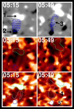
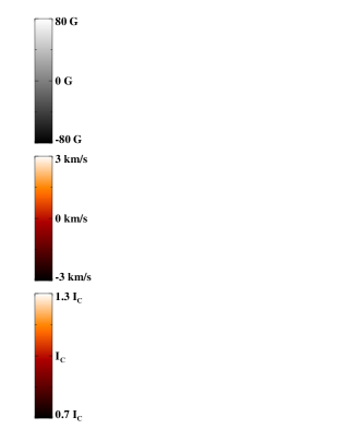
Figure 3: LOS magnetograms (region “I” in Fig. 1) in different time (the upper panels) with an emerging dipole being indicated by arrow “1” (positive) and arrow “2” (negative), corresponding Dopplergrams (the middle panels) and Ca ii H images (the bottom panels). The green and blue curves are contours of the positive ($+$80 G) and negative ($-$80 G) elements, respectively. The blue arrows show the transverse fields between the dipolar elements, while the dotted lines are contours of the Doppler blue shift ($-$2.0 km$/$s). Arrows “3” and “4” denote the place of a newly formed magnetic concentration. The I_c (same as in Figs. 4, 6, and 7) marked on the color bar represents the average value of Ca ii H intensities in the FOV of Ca ii H images.

Magnetic flux emergence is a main form of magnetic field evolution. Here, we study an emerging dipole at the CH boundary using the data from HINODE$/$SOT.

Figure 3 shows the region “I” in Fig. 1 in an expanded view. Two LOS magnetograms (the upper panels) display an emerging dipole being indicated by arrows “1” (positive) and “2” (negative). The blue arrows show the transverse magnetic fields between the dipolar elements, while the dotted lines are contours of the Doppler blue shift ($-$2.0 km$/$s). We can see that, the transverse fields between the dipolar elements point from the positive element to the negative one, and on the narrow zones where the transverse fields lie, there are strong blue shifts relative to the surrounding parts. In the bottom panels, the darker features on the Ca ii H images mainly coincide with the stronger blue shift places. Note that the break of the Doppler structure at 05:49 UT (indicated by arrow “4”) is caused by a newly emerged flux on the corresponding place (pointed by arrow “3”).

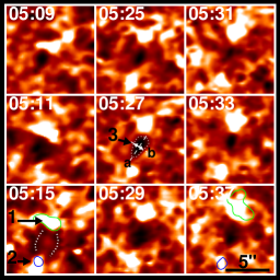
Figure 4: Sequence of Ca ii H images showing three developing processes of three mini AFs led by the emergence of the new dipole (see Fig. 3). The dipolar elements (indicated by arrows “1” and “2”) at 05:15 UT and 05:49 UT have been respectively contoured to the temporally nearest panels. Two thick dotted lines indicate two segments divided from the initial one. Arrow “3” denotes the main body of the AF (described with the thin dotted line). Line “a” is drawn along filament, while line “b” is perpendicular to line “a” and put at the midpoint of the intercept of “a” with the contour. Bi-head arrow expresses the width of the AF.

The chromospheric response to the emergence of that dipole is shown in Fig. 4. The sequence of Ca ii H images shows the development process of arch filaments (AFs). The dipolar elements (indicated by arrows “1” and “2”) at 05:15 UT and 05:49 UT have been respectively contoured to the temporally nearest panels. Three AFs have been observed in turn. Each column shows mainly the development of one AF. The first AF appeared at 05:07 UT and then expanded larger. At 05:09 UT, the AF looked like a dark absorption region. This AF expanded firstly and then divided into two segments. At 05:15 UT, the two segments connecting two brighter patches were much obvious. Comparing with SP magnetograms, we noticed that the bright patches in Ca ii were co-spatial with the concentrations of the magnetic field of both polarities. The two segments persisted for several minutes without obvious change in size. At 05:23 UT, another similar AF appeared at the same location as the previous one and began growing. Two minutes later, the AF was much more obvious seen in the image labeled with “05:25”. Then the AF erupted suddenly (at 05:29 UT) and dissipated quickly, so that it could not be distinguished from the background in the next image (at 05:31 UT). Arrow “3” denotes the main body of this AF (described with the thin dotted line). In a similar way to the middle column, the right shows the erupting process of the last AF. It emerged just following the eruption of the former one, continued expanding and erupted suddenly at 05:41 UT.

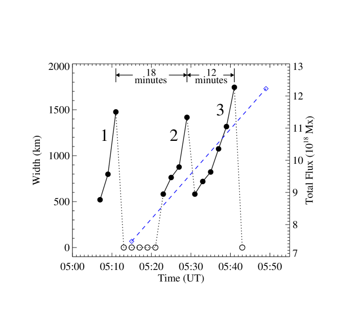
Figure 5: Temporal variation of the width (circle symbols) of the AFs and the total unsigned magnetic flux (diamonds) of the dipole. The solid line “1” (“2”$/$“3”) connecting the filled circles represents one visible dividing (erupting) process, while dotted lines indicate the invisible stages. When the AF divided or no AF could be distinguished from the background, the width is set to zero (unfilled circles). The dashed line represents the change of the total unsigned magnetic flux.

We measure the width (bi-head arrow in Fig. 4) of the AFs in each Ca II image and show the temporal evolution of the measured width with the filled circle symbols in Fig. 5. When the AF divided or no AF could be distinguished from the background, the width is set to zero and represented with unfilled circles. The solid line “1” (“2”$/$“3”) connecting the filled circles represents the visible width variation of an AF, while dotted lines indicate the invisible stages. The lifetimes of these three AF are 4, 6, 10 minutes and the two intervals between the three divisions or eruptions are 18 and 12 minutes, respectively. Also plotted in this figure is the total unsigned magnetic flux (connected with a dashed line) of the dipole, increasing from 7.48${\times}$10¹⁸ Mx to 1.22${\times}$10¹⁹ Mx in 34 minutes.

3.2 Magnetic flux emergence in the CH

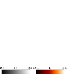
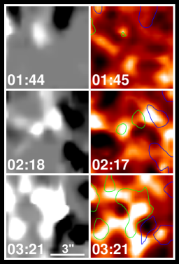
Figure 6: Example of IN flux emergence of mixed-polarity clusters (region “II” in Fig. 1). The left column shows LOS magnetograms, while the right column consists of Ca ii H images. Green and blue contours represent the positive and negative elements at $+$15 G and $-$15 G levels, respectively.

Except for the obvious dipolar emergence, we also find that many magnetic fluxes emerge in the form of mixed-polarity clusters. Figure 6 shows an example of IN flux emergence (region “II” in Fig. 1) in the CH. The left column shows LOS magnetograms, while the right one consists of Ca ii H images. Green and blue contours represent respectively the positive and negative magnetic elements at $+$15 G and $-$15 G levels. The total unsigned magnetic flux of this region increased from 5.17${\times}$10¹⁷ Mx (01:44 UT) to 1.24${\times}$10¹⁸ Mx (02:18 UT), then reached 2.47${\times}$10¹⁸ Mx (03:21 UT). On the other hand, we calculate the brightness of the Ca ii H line images and find it increased about 15% at 03:21 UT compared to that at 01:45 UT, exhibiting an increasing trend.

3.3 Magnetic flux cancellation at the CH boundary

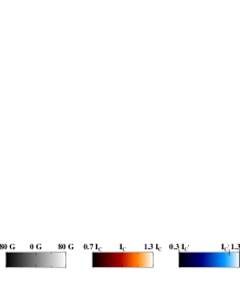
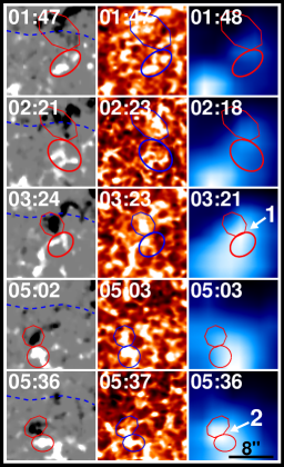
Figure 7: Example of NT flux cancellation locating at the CH boundary (region “III” in Fig. 1). Time sequence of LOS magnetograms (left column) shows the cancellations between one group of negative elements (outlined with octagons) and two groups of positive elements (outlined respectively with ellipses of thick and thin line) during their evolution. Dashed lines represent the boundary of the CH. Middle column images are the corresponding response of Ca ii H line, whereas right column ones 171 Å line. Note that the adjacent areas of the octagons and the ellipses are the places where the cancellations occur. Arrows “1” and “2” indicate the areas where much stronger cancellations take place. The I${}_{c^{\prime}}$ represents the average value of 171 Å intensities in the full-disk of 171 Å images.

Magnetic flux cancellation is another primary form of magnetic field evolution. In region “III” (see Fig. 1) that locates at the boundary of the CH, we observe the flux cancellations that occurred between one group of negative NT elements and two groups of positive ones in turn, as shown in Fig. 7. Left column shows a time sequence of magnetic field evolution. Dashed lines represent the CH boundary. The negative elements (outlined with octagons), initially locating in the CH, moved toward the boundary and cancelled partially with the positive elements (outlined with ellipses of thick lines) outside the CH. At 05:02 UT, the negative elements had become much smaller. They encountered another positive cluster (outlined with ellipses of thin lines) and interacted with it. Middle column images show the corresponding response of Ca ii H line, whereas right column 171 Å line. We can see that the bright points of Ca ii H are coincided well with the magnetic NT elements in locations, while the brighter regions seen in the 171 $\AA$ images only appear to coincide with the underlying magnetic elements when they are interacting.

As indicated by arrows “1” and “2” at 03:21 UT and 05:36 UT, much stronger cancellations took place with more obvious brightening of the upper atmosphere. The 171 $\AA$ brightness at the cancelling areas kept increasing during the two cancelling courses. At 03:21 UT and 05:36 UT, it increased respectively about 10% and 8% than that of pre-cancellation phase.

3.4 Magnetic flux distribution in the CH

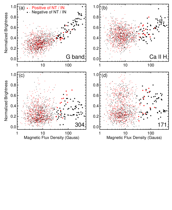
Figure 8: Relationship between the normalized brightness of the images of different wavelengths and the absolute values of the magnetic flux densities. The big (small) red and black dots represent the positive and negative data of the NT (IN) elements, respectively.

Besides the above case studies of the atmospheric response to the magnetic field evolution, we have investigated the relations between the distribution of magnetic flux and brightness at different atmospheric layers in the CH (only the common part of the SP and BFI FOVs). We measure the magnetic flux of each NT and IN element in the LOS magnetogram obtained from 04:51 UT to 05:23 UT and the brightness of the corresponding images of several spectral lines. In order to compare the results of both negative and positive elements, two kinds of them are measured separately. For the NT fields, 66 negative and 14 positive elements are identified and measured, and the total magnetic flux is $-$1.85$\times$10²⁰ Mx and 0.21$\times$10²⁰ Mx, respectively. We also measure 593 negative and 571 positive IN elements, and the total flux is $-$0.97$\times$10²⁰ Mx and 0.78$\times$10²⁰ Mx, respectively. Then we deduce the average magnetic flux density and brightness of each element.

Figure 8 shows the relationship between the normalized brightness and the magnetic flux densities. The big (small) red and black dots represent the positive and negative NT (IN) elements, respectively. Figure 8a demonstrates that there exists a high positive correlation between the G band brightness and the magnetic flux density for the NT elements. If two polarities are synthetically considered, the linear correlation for the NT will be as high as 0.85. We also calculate the linear correlation coefficient for the IN and find it is only 0.27. Figure 8b exhibits a linear correlation for the NT of the Ca ii H, only distinguished from that of G band with a lower correlation coefficient (0.58). But neither the positive nor the negative IN has this type of trend. Then Fig. 8c (8d) displays no correlation between the 304 Å (171 Å) brightness and the magnetic flux densities for both the NT and the IN. The results of 195 Å and 284 Å are similar to Figs. 8c$-$d.

4 Conclusions and discussion

We have investigated an equatorial CH and its boundary region observed simultaneously by HINODE and STEREO on July 27, 2007. With the help of the vector magnetic fields and the Dopplergrams, we study an emerging dipole locating at the CH boundary. Three AFs accompanying the dipole appeared and expanded in turn, observed with Ca ii H line. The first AF divided into two segments in its late stage. The second and third AFs erupted and diffused with an extremely rapid speed in their late stages. The lifetimes of these three AFs are 4, 6, 10 minutes, and the two intervals between the three divisions or eruptions are 18 and 12 minutes, respectively. We display an example of mixed-polarity flux emergence of IN fields within the CH and present the corresponding chromospheric response. With the increase of the integrated magnetic flux, the brightness of the Ca ii H images exhibits an increasing trend. In addition, we also study magnetic flux cancellations of NT fields locating at the CH boundary and present the obvious chromospheric and coronal response. By examining the magnetic NT and IN elements and the response of different atmospheric layers, we find there exists a good positive linear correlation (correlation coefficient 0.8) between the G band brightness and the magnetic flux density for the NT. The correlation coefficient for the IN of G band is much lower, only 0.27. We also obtain good linear correlation ( correlation coefficient 0.58) for the NT of Ca ii H line.

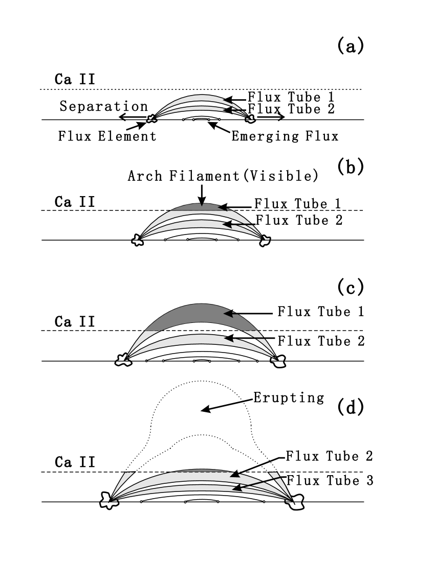
Figure 9: Cartoons illustrating the multi-erupting process of the small-scale AFS. Dashed lines indicate the lower limit where the Ca ii H line is formed. In phase “a”, there is no visible AF at the moment because all the magnetic flux tubes are too low to be observed with Ca ii H line. Then the tubes rise and part of flux tube 1 begins to be observed as AF (darker part), as shown in phase “b”. From phase “b” to phase “c”, tube 1 continues to rise and expand, so the AF apparently becomes bigger. In the late stage (phase “d”), the AF erupts suddenly due to some physical mechanism and gets optically thin and invisible instantly within the visible region of the Ca ii H line, following which another developing and erupting process for flux tube 2 begins.

In order to illustrate the intermittent appearance and eruptions of the AFs, a series of cartoons (see Fig. 9) are sketched out, based on the previous model provided by Frazier (1972). The process of the multi-eruptions can be decomposed into four phases (Figs. 9a$-$d). Dashed lines indicate the lower limit where the Ca ii H line is formed. In Fig. 9a, there is no visible AF at the moment because all the magnetic flux tubes are too low to be observed with Ca ii H line. Then the tubes rise and part of flux tube “1” begins to be observed as an AF (darker part) (Fig. 9b). Tube “1” continues to rise and expand, so the AF apparently becomes bigger (Fig. 9c). In the late stage (Fig. 9d), the AF erupts suddenly due to some physical mechanism and gets optically thin and invisible instantly within the visible region of the Ca ii H line, following which another AF develops. In each phase, the dipolar footpoints separate persistently, accompanied with new flux emerging.

Yamauchi et al. (2005) have studied the eruptions of mini-filaments, running nearly parallel to the neutral lines and crossing them with small angles, in a CH. A filament, exhibited in an example, erupted and rose to a high level where its top was invisible. Then a new visible filament formed along the initial path of the erupted one. Similarly, rising rapidly to an excessive height above the layer where the Ca ii H line is formed may be the cause of the invisibility of AFs in their late stages reported in this paper, no matter whether they are optically thin or not.

CH boundaries separate the CHs from the surrounding quiet regions and play crucial roles in the evolution of the CHs. Kahler & Hudson (2002; see also Dahlburg & Einaudi 2003) have researched the magnetic morphology of CH boundaries. These studies are helpful to understand the rigid rotation which is most likely correlated with the processes occurring at the boundaries (Nash et al. 1988; Wang & Sheeley 1990, 2004; Fisk et al. 1999; Fisk & Schwadron 2001). In order to maintain the integrity of the CHs, magnetic reconnection must occur continuously at the boundaries (Wang et al. 1996; Kahler & Hudson 2002). Wang et al. (1996) and Schwadron et al. (1999) suggested that there exists magnetic reconnection between the open field lines and the adjacent closed ones along the boundaries. The evidence for such reconnection was revealed with the existence of bidirectional jets by Madjarska et al. (2004) for the first time. Then more direct evidence was given by Raju et al. (2005) and Baker et al. (2007). When magnetic reconnection occurs, the magnetic field is restructured accompanied with energy release (e.g. bright point appears in EUV image); meanwhile small loop forms and submerges leading to an observational phenomenon $-$ magnetic flux cancellation, just as shown in Fig. 7 (see also Wang & Shi 1993; Zhang et al. 2001, 2007).

Our result that there are good positive linear correlations between the NT magnetic flux densities and the brightness of both G band and Ca ii H in the CH is consistent with the research of Zirin (1988) and Nindos & Zirin (1998) in the QS. The lower correlation for the NT of Ca ii H than of G band can be considered to be caused by the fact that, when the flux tubes extend to the chromosphere, they expand, becoming larger than in the photosphere. With the increase of the height, the flux tubes enlarge quite a lot and most of them change their directions. Especially in the corona, the average expansion factor (ratio of the maximum to the minimum of the flux tube area) is 28 ${\pm}$ 11 (Wiegelmann et al. 2005). The decline and expansion of the flux tubes can be used to interpret why there is no correlation in the transition region and the corona (exhibited by Figs. 8c and 8d), although the relatively lower tempo-spatial resolution of the images from STEREO may be one cause.

The large part of scatter of the data points for the IN of Ca ii H in Fig. 8b is mainly due to the 3-min oscillations, which does not permit us to obtain a correlation between the brightness and magnetic fields even if it exists on the Sun (Sivaraman et al. 2000). The low correlation coefficient (0.27) for the IN of G band in Fig. 8a also may be affected by the 3-min oscillations. Another reason for the lack of obvious linear correlation for both G band and Ca ii H IN may be that the cadence of G band and Ca images is not high enough. The average lifetime of the IN elements is only about 4.84 minutes (Zhou, G. private communication), so lots of the magnetic IN elements have evolved quite a lot within one minute. The same reasons can also explain why there is only partial coincidence between the magnetic elements and the bright features shown in Fig. 6. While the poor correlations for the IN of 304 Å, 171 Å, 195 Å and 284 Å lines are mainly due to the lower tempo-spatial resolution of the images and the incapability of the IN flux tubes to extend into the transition region and the corona (Wiegelmann & Solanki 2004; Wiegelmann et al. 2005).

- (1) Akinari, N. 2007, ApJ, 660, 1660
- (2) Alissandrakis, C. E., Tsiropoula, G., & Mein, P. 1990, A&A, 230, 200
- (3) Baker, D., van Driel-Gesztelyi, L., & Attrill, G. D. R. 2007, Astron. Nachr., 328, 773
- (4) Beck, C., Schmidt, W., Rezaei, R., & Rammacher, W. 2008, A&A, 479, 213
- (5) Belenko, I. A. 2001, Sol. Phys., 199, 23
- (6) Bilenko, I. A. 2002, A&A, 396, 657
- (7) Bilenko, I. A. 2004, Sol. Phys., 221, 261
- (8) Bohlin, J. D. 1977, Sol. Phys., 51, 377
- (9) Bruzek, A. 1967, Sol. Phys., 2, 451
- (10) Bruzek, A. 1969, Sol. Phys., 8, 29
- (11) Carlsson, M., Stein, R. F., Nordlund, Å., & Scharmer, G. B. 2004, ApJ, 610, L137
- (12) Chou, D. Y. 1993, In: Zirin, H., Ai, P., Wang, H. (eds.) ASP conf. series vol. 46, p. 471
- (13) Chou, D. Y., & Zirin, H. 1988, ApJ, 333, 420
- (14) Cranmer, S. R. 2002, Space Sci. Rev., 101, 229
- (15) Crooker, N. U., & Cliver, E. W. 1994, J. Geophys. Res., 99, 23383
- (16) Dahlburg, R. B., & Einaudi, G. 2003, Adv. Space Res., 32, 1125
- (17) Delaboudinière, J. P., Artzner, G. E., Brunaud, J., et al. 1995, Sol. Phys., 162, 291
- (18) Domingo, V., Fleck, B., & Poland, A. I. 1995, Sol. Phys., 162, 1
- (19) Dowdy, J. F. 1993, ApJ, 411, 406
- (20) Dowdy, J. F., Rabin, D., & Moore, R. L. 1986, Sol. Phys., 105, 35
- (21) Dwivedi, B. N., & Srivastava, A. K. 2006, Sol. Phys., 237, 143
- (22) Feldman, U., & Laming, J. M. 2000, Phys. Scr, 61, 222
- (23) Feldman, U., Dammasch, I. E., & Wilhelm, K. 2001, ApJ, 558, 423
- (24) Fisk, L. A., & Schwadron, N. A. 2001, ApJ, 560, 425
- (25) Fisk, L. A., Zurbuchen, T. H., & Schwadron, N. A. 1999, ApJ, 521, 868
- (26) Frazier, E. N. 1970, Sol. Phys., 14, 89
- (27) Frazier, E. N. 1972, Sol. Phys., 26, 130
- (28) Georgaklilas, A. A., Alissandrakis, C. E., & Zachariadis, T. G. 1990, Sol. Phys., 129, 277
- (29) Giordano, S., Antonucci, E., Noci, G., et al. 2000, ApJ, 531, L79
- (30) Hackenberg, P., Marsch, E., & Mann, G. 2000, A&A, 360, 1139
- (31) Harvey, J. W., & Sheeley, N. R. 1979, Space Sci. Rev., 23, 139
- (32) Harvey, K. L. 1996, in AIP Conf. Ser. 382, Proc. Eighth International Solar Wind Conference, ed. D. Winterhalter et al. (New York: AIP), 9
- (33) Harvey, K. L., & Recely, F. 2002, Sol. Phys., 211, 31
- (34) Hofer, M. Y., & Storini, M. 2002, Sol. Phys., 207, 1
- (35) Howard, R. A., Moses, J. D., Vourlidas, A., et al. 2008, Space Sci. Rev., 136, 67
- (36) Ichimoto, K., Lites, B., Elmore, D., et al. 2008, Sol. Phys., 249, 233
- (37) Janse, Å. M., Lie-Svendsen, Ø., & Leer, E. 2007, A&A, 474, 997
- (38) Jordan, C., Macpherson, K. P., & Smith, G. R. 2001, MNRAS, 328, 1098
- (39) Kahler, S. W., & Hudson, H. S. 2002, ApJ, 574, 467
- (40) Kaiser, M. L., Kucera, T. A., Davila, J. M., et al. 2008, Space Sci. Rev., 136, 5
- (41) Kobanov, N. I., & Sklyar, A. A. 2007, Astron. Rep., 51, 773
- (42) Kobanov, N. I., Makarchik, D. V., & Sklyar, A. A. 2003, Sol. Phys., 217, 53
- (43) Kosugi, T., Matsuzaki, K., Sakao, T., et al. 2007, Sol. Phys., 243, 3
- (44) Krieger, A. S., Timothy, A. F., & Roelof, E. C. 1973, Sol. Phys., 29, 505
- (45) Laming, J. M., & Feldman, U. 2003, ApJ, 591, 1257
- (46) Leighton, R. B. 1959, ApJ, 130, 366
- (47) Leighton, R. B., Noyes, R. W., & Simon, G. W. 1962, ApJ, 135, 474
- (48) Levine, R. H. 1977, ApJ, 218, 291
- (49) Lites, B. W., Elmore, D. F., & Streander, K. V. 2001, in ASP Conf. Ser. 236, Advanced Solar Polarimetry-Theory, Observation, and Instrumentation, ed. M. Sigwarth (San Francisco: ASP), 33
- (50) Lites, B. W., Rutten, R. J., & Berger, T. E. 1999, ApJ, 517, 1013
- (51) Livingston, W. C., & Harvey, J. 1975, BAAS, 7, 346
- (52) Madjarska, M. S., Doyle, J. G., & van Driel-Gesztelyi, L. 2004, ApJ, 603, L57
- (53) Mahajan, S. M., Miklaszewski, R., Nikol’Skaya, K. I., & Shatashvili, N. L. 2002, Adv. Space. Res., 30, 545
- (54) Maravilla, D., Lara, A., Valdés Galicia, J. F., & Mendoza, B. 2001, Sol. Phys., 203, 27
- (55) Markovskii, S. A., & Hollweg, J. V. 2004, ApJ, 609, 1112
- (56) Meunier, N. 2005, A&A, 443, 309
- (57) Moran, T. G. 2003, ApJ, 598, 657
- (58) Munro, R. H., & Withbroe, G. L. 1972, ApJ, 176, 511
- (59) Nash, A. G., Sheeley, N. R., & Wang, Y. M. 1988, Sol. Phys., 117, 359
- (60) Nindos, A., & Zirin, H. 1998, Sol. Phys., 179, 253
- (61) O’Shea, E., Banerjee, D., & Doyle, J. G. 2005, A&A, 436, L35
- (62) O’Shea, E., Banerjee, D., & Doyle, J. G. 2006, A&A, 452, 1059
- (63) O’Shea, E., Banerjee, D., & Doyle, J. G. 2007, A&A, 463, 713
- (64) Patsourakos, S., & Vial, J. C. 2000, A&A, 359, L1
- (65) Patsourakos, S., Habbal, S. R., & Hu, Y. Q. 2002, ApJ, 581, L125
- (66) Raju, K. P., Bromage, B. J. I., Chapman, S. A., & Del Zanna, G. 2005, A&A, 432, 341
- (67) Raju, K. P., Sakurai, T., Ichimoto, K., & Singh, J. 2000, ApJ, 543, 1044
- (68) Reeves, E. M., & Parkinson, W. H. 1970, ApJS, 21, 1
- (69) Reeves, E. M., Timothy, J. G., & Huber, M. C. E. 1977, Appl. Opt., 16, 837
- (70) Remling, B., Deubner, F. L., & Steffens, S. 1996, A&A, 316, 196
- (71) Rezaei, R., Schlichenmaier, R., Beck, C. A. R., et al. 2007, A&A, 466, 1131
- (72) Scherrer, P. H., Bogart, R. S., Bush, R. I., et al. 1995, Sol. Phys., 162, 129
- (73) Schwadron, N. A., Fisk, L. A., & Zurbuchen, T. H. 1999, ApJ, 521, 859
- (74) Shen, C. L., Wang, Y. M., Ye, P. Z., & Wang, S. 2006, ApJ, 639, 510
- (75) Shimizu, T., Nagata, S., Tsuneta, S., et al. 2008, Sol. Phys., 249, 221
- (76) Sivaraman, K. R., & Livingston, W. C. 1982, Sol. Phys., 80, 227
- (77) Sivaraman, K. R., Gupta, S. S., Livingston, W. C., et al. 2000, A&A, 363, 279
- (78) Skumanich, A., Smythe, C., & Frazier, E. N. 1975, ApJ, 200, 747
- (79) Srivastava, A. K., & Dwivedi, B. N. 2007, JA&A, 28, 1
- (80) Steffens, S., Hofmann, J., & Deubner, F. L. 1996, A&A, 307, 288
- (81) Stenflo, J. O., & Harvey, J. W. 1985, Sol. Phys., 95, 99
- (82) Stepanian, N. N. 1995, Izv. Ross. Akad. Nauk, Ser. Fiz., 59(7), 63
- (83) Stucki, K., Solanki, S. K., Pike, C. D., et al. 2002, A&A, 381, 653
- (84) Stucki, K., Solanki, S. K., Schühle, U., et al. 2000, A&A, 363, 1145
- (85) Suematsu, Y., Tsuneta, S., Ichimoto, K., et al. 2008, Sol. Phys., 249, 197
- (86) Temmer, M., Vršnak, B., & Veronig, A. M. 2007, Sol. Phys., 241, 371
- (87) Teplitskaya, R. B., Turova, I. P., & Ozhogina, O. A. 2007, Sol. Phys., 243, 143
- (88) Teriaca, L., Poletto, G., Romoli, M., & Biesecker, D. A. 2003, ApJ, 588, 566
- (89) Tian, H., Marsch, E., Tu, C. Y., et al. 2008, A&A, 482, 267
- (90) Tsiropoula, G., Georgakilas, A. A., Alissandrakis, C. E., & Mein, P. 1992, A&A, 262, 587
- (91) Tsuneta, S., Ichimoto, K., Katsukawa, Y., et al. 2008, Sol. Phys., 249, 167
- (92) Tsurutani, B. T., & Gonzalez, W. D. 1987, Planet. Space Sci., 35, 405
- (93) Tu, C. Y., Zhou, C., Marsch, E., et al. 2005, Sci, 308, 519
- (94) Underwood, J. H., & Muney, W. S. 1967, Sol. Phys., 1, 129
- (95) Vernazza, J. E., Avrett, E. H., & Loser, R. 1981, ApJS, 45, 635
- (96) Veronig, A. M., Temmer, M., Vršnak, B., & Thalmann, J. K. 2006, ApJ, 647, 1466
- (97) Vršak, B., Temmer, M., & Veronig, A. M. 2007, Sol. Phys., 240, 315
- (98) Waldmeier, M. 1951, ZAp, 30, 1
- (99) Wang, J. X., & Shi, Z. X. 1993, Sol. Phys., 143, 119
- (100) Wang, Y. M., & Sheeley, N. R. 1990, ApJ, 365, 372
- (101) Wang, Y. M., & Sheeley, N. R. 2004, ApJ, 612, 1196
- (102) Wang, Y. M., Hawley, S. H., & Sheeley, N. R. 1996, Sci, 271, 464
- (103) Warren, H. P., & Winebarger, A. R. 2000, ApJ, 535, L63
- (104) Weart, S. R. 1970, ApJ, 162, 987
- (105) Wiegelmann, T., & Solanki, S. K. 2004, Sol. Phys., 225, 227
- (106) Wiegelmann, T., Xia, L. D., & Marsch, E. 2005, A&A, 432, L1
- (107) Wilhelm, K. 2006, A&A, 455, 697
- (108) Wilhelm, K., Dammasch, I. E., & Xia, L. D. 2002, Adv. Space Res., 30, 517
- (109) Wilhelm, K., Dammasch, I. E., Marsch, E., & Hassler, D. M. 2000, A&A, 353, 749
- (110) Worden, J., Harvey, J., & Shine, R. A. 1999, ApJ, 523, 450
- (111) Wu, D. J., & Yang, L. 2007, ApJ, 659, 1693
- (112) Xia, L. D., Marsch, E., & Curdt, W. 2003, A&A, 399, L5
- (113) Xia, L. D., Marsch, E., & Wilhelm, K. 2004, A&A, 424, 1025
- (114) Yamauchi, Y., Moore, R. L., Suess, S. T., et al. 2004, ApJ, 605, 511
- (115) Yamauchi, Y., Wang, H., Jiang, Y., et al. 2005, ApJ, 629, 572
- (116) Zhang, J., Li, L. P., & Song, Q. 2007, ApJ, 662, L35
- (117) Zhang, J., Lin, G. H., Wang, J. X., et al. 1998a, A&A, 338, 322
- (118) Zhang, J., Lin, G. H., Wang, J. X., et al. 1998b, Sol. Phys., 178, 245
- (119) Zhang, J., Ma, J., & Wang, H. M. 2006, ApJ, 649, 464
- (120) Zhang, J., Wang, J. X., Deng, Y. Y., & Wu, D. J. 2001, ApJ, 548, L99
- (121) Zhang, J., Wang, J. X., Wang, H. M., & Zirin, H. 1998c, A&A, 335, 341
- (122) Zhang, J., Woch, J., & Solanki, S. 2005a, Chinese J. Astron. Astrophys., 5, 531
- (123) Zhang, J., Woch, J., Solanki, S. K., & von Steiger, R. 2002, Geochim. Res. Lett., 29, 1236
- (124) Zhang, J., Woch, J., Solanki, S. K., et al. 2003, J. Geophys. Res., 108, 1144
- (125) Zhang, J., Zhou, G. P., Wang, J. X., & Wang, H. M. 2007, ApJ, 655, L113
- (126) Zhang, T. X. 2003, ApJ, 597, L69
- (127) Zhang, T. X., Wang, J. X., & Xiao, C. J. 2005b, Chinese J. Astron. Astrophys., 5, 285
- Zirker (1977) Zirin, H. 1988, Astrophysics of the Sun, Cambridge University Pres, Cambridge
- Zirker (1977) Zirker, J. B., ed. 1977, Coronal Holes and High-Speed Wind Streams (Boulder: Colorado Associated Univ. Press)