The Context Sensitivity Problem in Biological Sequence Segmentation

Abstract

In this paper, we describe the context sensitivity problem encountered in partitioning a heterogeneous biological sequence into statistically homogeneous segments. After showing signatures of the problem in the bacterial genomes of Escherichia coli K-12 MG1655 and Pseudomonas syringae DC3000, when these are segmented using two entropic segmentation schemes, we clarify the contextual origins of these signatures through mean-field analyses of the segmentation schemes. Finally, we explain why we believe all sequence segmentation schems are plagued by the context sensitivity problem.

I Introduction

Biological sequences are statistically heterogeneous, in the sense that local compositions and correlations in different regions of the sequences can be very different from one another. They must therefore treated as collections of statistically stationary segments (or domains), to be discovered by the various segmentation schemes found in the literature (see review by Braun and Müller [1], and list of references in Ref. 2). Typically, these segmentation schemes are tested on (i) artificial sequences composed of a small number of segments, (ii) control sequences obtained by concatenating known coding and noncoding regions, or (iii) control sequences obtained by concatenating sequences from chromosomes know to be statistically distinct. They are then applied on a few better characterized genomic sequences, and compared against each other, to show general agreement, but also to demonstrate better sensitivity in delineating certain genomic features. To the best of our knowledge, there are no studies reporting a full and detailed comparison of the segmentation of a sequence against its distribution of carefully curated gene calls. There are also no studies comparing the segmentations of closely related genomes. In such sequences, there are homologous stretches, interrupted by lineage specific regions, and the natural question is whether homologous regions in different genomes will be segmented in exactly the same way by the same segmentation scheme.

In this paper, we answer this question, without comparing the segmentation of homologous regions. Instead, through careful observations of how segment boundaries, or domain walls, are discovered by two different entropic segmentation schemes, we realized that a subsequence can be segmented differently by the same scheme, if it is part of two different full sequences. We call this dependence of a segmentation on the detailed arrangement of segments the context sensitivity problem. In Sec. II, we will describe how the context sensitivity problem manifests itself in real genomes, when these are segmented using a sliding-window entropic segmentation scheme, which examines local contexts in the sequences, versus segmentation using a recursive entropic segmentation scheme, which examines the global contexts of the sequences. We then show how the context sensitivity problem prevents us from coarse graining by using larger window sizes, stopping recursive segmentation earlier, or by simply removing weak domain walls from a fine-scale segmentation. We follow up in Sec. III with a mean-field analysis of the local and global context sensitivity problems, showing how the positions and strengths of domain walls, and order in which these are discovered, are affected by these contexts. In particular, we identify repetitive sequences as the worst case scenario to encounter during segmentation. Finally, in Sec. IV, we summarize and discuss the impacts of our findings, and explain why we believe the context sensitivity problem plagues all segmentation schemes.

II Context Sensitivity Problem in Real Bacterial Genomes

In this section, we investigate the manifestations of the context sensitivity problem in two real bacterial genomes, those of Escherichia coli K-12 MG1655 and Pseudomonas syringae DC3000, when these are segmented using two entropic segmentation schemes. The first entropic segmentation scheme, based on statistics comparison of a pair of sliding windows, is sensitive to the local context of segments within the pair of sliding windows, and we shall show in Sec. II-A that the positions and strengths of domain walls discovered by the scheme depends sensitively on the window size. The second entropic segmentation scheme is recursive in nature, adding new domain walls at each stage of the recursion. We shall show in Sec. II-B that this scheme is sensitive to the global context of segments within the sequence, and that domain walls are not discovered according to their true strengths. In Sec. II-C, we show that there is no statistically consistent way to coarse grain a segmentation by removing the weakest domain walls, and agglomerating adjacent segments.

II-A Paired Sliding Windows Segmentation Scheme

Using the paired sliding windows segmentation scheme described in App. -B, the number $M$ of order-$K$ Markov-chain segments discovered depends on the size $n$ of the windows used, as shown in Table I for E. coli K-12 MG1655. Because $M$ decreases as $n$ is increased, we are tempted to think that we can change the granularity of the segmental description of a sequence by tuning $n$, such that there are more and shorter segments when $n$ is made smaller, while there are fewer and longer segments when $n$ is made larger. Thus, as $n$ is increased, we expect groups of closely spaced domain walls to be merged as the short segments they demarcate are agglomerated, and be replaced by a peak close to the position of the strongest peak.

TABLE I: Number of $K=0$ domain walls in the E. coli K-12 MG1655 genome ($N=4639675$ bp), obtained using the paired sliding window segmentation scheme for different window sizes $1000\leq n\leq 5000$.

$n$	1000	2000	3000	4000	5000
$M$	2781	1414	952	721	577

Indeed, we do find this expected merging of proximal domain walls in Fig. 1 and Fig. 2, which shows the square deviation spectra for the $(0,40000)$ region of the E. coli K-12 MG1655 genome and the $(25000,75000)$ region of the P. syringae DC3000 genome respectively. In the $(0,40000)$ region of the E. coli K-12 MG1655 genome shown in Fig. 1, we find the group of domain walls, $i_{a}\approx 16500$, $i_{b}\approx 17500$, and $i_{c}\approx 18700$, and the pair of domain walls, $i_{g}\approx 33800$ and $i_{h}\approx 35000$, which are distinct in the $n=1000$ square deviation spectrum, merging into the domain walls $i_{abc}$ and $i_{gh}$ in the $n\geq 3000$ square deviation spectra. In the $(25000,75000)$ region of the P. syringae DC3000 genome shown in Fig. 2, we find the pair of domain walls, $j_{a}\approx 45000$ and $j_{b}\approx 46600$, and the pair of domain walls, $j_{c}\approx 50400$ and $j_{d}\approx 51800$, which are distinct in the $n=1000$ square deviation spectrum, merging into the domain walls $j_{ab}$ and $j_{cd}$ in the $n\geq 3000$ and $n=5000$ square deviation spectra respectively.

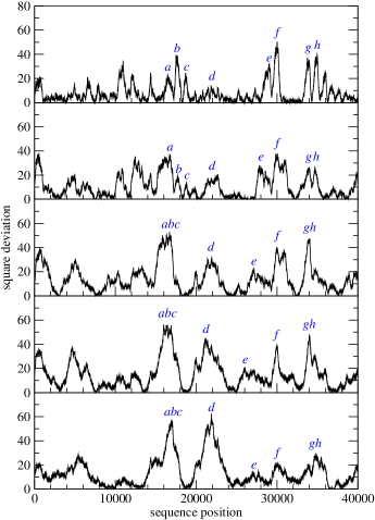
Figure 1: The $K=0$ square deviation spectra in the region $(0,40000)$ of the E. coli K-12 MG1655 genome, obtained using the paired sliding window segmentation scheme with window sizes (top to bottom) $n=1000$, 2000, 3000, 4000, and 5000.

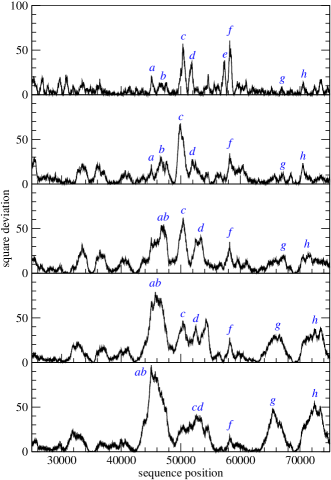
Figure 2: The $K=0$ square deviation spectra in the region $(25000,75000)$ of the P. syringae DC3000 genome, obtained using the paired sliding window segmentation scheme with window sizes (top to bottom) $n=1000$, 2000, 3000, 4000, and 5000.

However, we also find unexpected changes in the relative strengths of the domain walls, as $n$ is increased. In the $(0,40000)$ region of the E. coli K-12 MG1655 genome shown in Fig. 1, we find that $i_{d}\approx 21800$, which appears as a broad, weak, and noisy bump in the $n=1000$ square deviation spectrum, becoming stronger and more defined as $n$ is increased, and finally becomes as strong as the domain wall $i_{abc}$ in the $n=5000$ square deviation spectrum. In this region of the E. coli K-12 MG1655 genome, we also find that the domain walls $i_{b}\approx 17500$ and $i_{f}\approx 30000$ are equally strong in the $n=1000$ square deviation spectrum, but as $n$ is increased, $i_{b}$ becomes stronger while $i_{f}$ becomes weaker. In the $(25000,75000)$ region of the P. syringae DC3000 genome shown in Fig. 2, we find that the domain walls $j_{c}\approx 50400$ and $j_{f}\approx 58200$ are equally strong, and also the domain walls $j_{d}\approx 51800$ and $j_{e}\approx 57300$ are equally strong, in the $n=1000$ square deviation spectrum. However, as $n$ is increased, $j_{c}$ becomes stronger than $j_{f}$, while $j_{d}$ becomes stronger than $j_{e}$. More importantly, all these domain walls — the strongest in this $(25000,75000)$ region of the $n=1000$ square deviation spectrum — become weaker as $n$ is increased, to be superseded by the domain walls $j_{ab}\approx 45000$, $j_{g}\approx 65400$ and $j_{h}\approx 72400$, which become stronger as $n$ is increased. As it turned out, $(j_{c},j_{f})$ overlaps significantly with the interval interval $(50000,59000)$, which incorporates three lineage-specific regions (LSRs 5, 6, and 7, all of which virulence related) identified by Joardar et al [3]. It is therefore biologically significant that $j_{c}$ and $j_{f}$ are strong domain walls in the $n=1000$ square deviation spectrum. On the other hand, it is not clear what kind of biological meaning we can attach to $j_{ab}$, $j_{g}$, and $j_{h}$ being the strongest domain walls in the $n=5000$ square deviation spectrum.

TABLE II: Positions of strong domain walls in the $(0,40000)$ region of the E. coli K-12 MG1655 genome and the $(25000,75000)$ region of the P. syringae DC3000 genome, determined after match filtering the square deviation spectra obtained using the paired sliding window segmentation scheme with window sizes $n=3000,4000,5000$.

	E. coli K-12 MG1655			P. syringae DC3000
$n$	$i_{abc}$	$i_{d}$	$i_{h}$	$j_{ab}$	$j_{g}$	$j_{h}$
3000	16200	21800	34100	46600	66600	71500
4000	16300	21700	34400	45900	65900	72500
5000	16100	22100	34700	45700	65500	72500

There is another, more subtle, effect that increasing the size of the sliding windows has on the domain walls: their positions, as determined from peaks in the square deviation spectrum after match filtering, are shifted. The shifting positions of some of the strong domain walls in the $(0,40000)$ region of the E. coli K-12 MG1655 genome and the $(25000,75000)$ region of the P. syringae DC3000 genome are shown in Table II. In general, the positions and strengths of domain walls can change when the window size used in the paired sliding windows segmentation scheme is changed, because windows of different sizes examine different local contexts. As a result of this local context sensitivity, whose nature we will illustrate using a mean-field picture in Sec. III-A, the sets of strong domain walls determined using two different window sizes $n$ and $n^{\prime}>n$ are different. If $n$ and $n^{\prime}$ are sufficiently different, the sets of strong domain walls, i.e. those stronger than a specified cutoff, may have very little in common. Therefore, we cannot think of the segmentation obtained at window size $n^{\prime}$ as the coarse grained version of the segmentation obtained at window size $n$.

II-B Optimized Recursive Jensen-Shannon Segmentation Scheme

Using the optimized recursive Jensen-Shannon segmentation scheme described in Ref. 2, we obtained one series of segmentations each for E. coli K-12 MG1655 and P. syringae DC3000, shown in Fig. 3 and Fig. 4 respectively. Two features are particularly striking about these plots. First, there exist domain walls stable with respect to segmentation optimization. These stable domain walls remain close to where they were first discovered by the optimized recursive segmentation scheme. Second, there are unstable domain walls that get shifted by as much as 10% of the total length of the genome when a new domain wall is introduced. For example, in Fig. 3 for the E. coli K-12 MG1655 genome, we find the domain wall $i_{10}=4051637$ in the optimized segmentation with $M=10$ domain walls shifted to $i_{10}=4469701$ in the optimized segmentation with $M=11$ domain walls ($\delta i_{10}=+418064$), and also the domain wall $i_{7}=2135183$ in the optimized segmentation with $M=15$ domain walls shifted to $i_{7}=2629043$ in the optimized segmentation with $M=16$ domain walls ($\delta i_{7}=+493860$). Based on the observation that some unstable domain walls are discovered, lost, later rediscovered and become stable, we suggested in Ref. 2 that for a given segmentation with $M$ domain walls, stable domain walls are statistically more significant than unstable domain walls, while stable domain walls discovered earlier are more significant than stable domain walls discovered later in the optimized recursive segmentation.

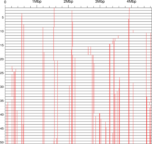
Figure 3: Series of optimized recursive Jensen-Shannon segmentations of the E. coli K-12 MG1655 genome, for (top to bottom) $2\leq M\leq 50$ domain walls. The two stable domain walls that appear in the $M=2$ optimized segmentation are close to the replication origin and replication terminus.

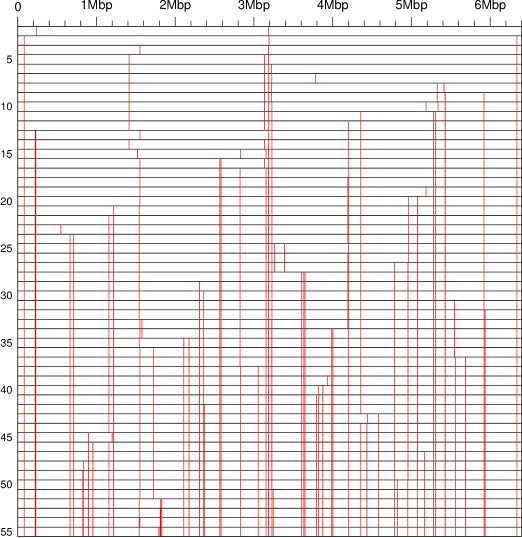
Figure 4: Series of optimized recursive Jensen-Shannon segmentations of the P. syringae DC3000 genome, for (top to bottom) $2\leq M\leq 55$ domain walls. Compared to the E. coli K-12 MG1655 genome, there are perceptibly more unstable domain walls in the P. syringae DC3000 genome.

From Fig. 3 and Fig. 4, we also find that the E. coli K-12 MG1655 and P. syringae DC3000 genomes have very different segmental textures. At this coarse scale ($M\sim 50$ segments), we find many short segments, many long segments, but few segments of intermediate lengths in the E. coli K-12 MG1655 genome. In contrast, at the same granularity, the P. syringae DC3000 genome contains many short segments, many segments of intermediate lengths, but few long segments. We believe these segmental textures are consistent with the different evolutionary trajectories of the two bacteria. E. coli K-12 MG1655, which resides in the highly stable human gut environment, has a more stable genome containing fewer large-scale rearrangements which appear to be confined to hotspots within the $(2600000,3600000)$ region. The genome of P. syringae DC3000, on the other hand, has apparently undergone many more large-scale rearrangements as its lineage responded to multiple evolutionary challenges living in the hostile soil environment.

We find many more large shifts in the optimized domain wall positions in P. syringae DC3000 compared to E. coli K-12 MG1655, because of the more varied context of the P. syringae DC3000 genome. However, large shifts in the optimized domain wall positions arise generically in all bacterial genomes, because of the sensitivity of optimized domain wall positions to the contexts they are restricted to. In Sec. III-B, we will illustrate using a mean-field picture how the recursive segmentation scheme decides where to subdivide a segment, i.e. add a new domain wall, after examining the global context within the segment. We then show how this global context changes when the segment is reduced or enlarged during segmentation optimization, which can then cause a large shift in the position of the new domain wall. Because of this global context sensitivity, we find in Fig. 4 a large shift of the domain wall $j_{9}=1723734$, which is stable when there are $36\leq M\leq 51$ optimized domain walls in the segmentation, to its new position $j_{9}=1818461$ ($\delta j_{9}=+94727$) when one more optimized domain wall is added. We say that a domain wall is stable at scale $M$ if it is only slightly shifted, or not at all, within the optimized segmentations with between $M-\delta M$ and $M+\delta M$ domain walls, where $\delta M\ll M$. Given a series of recursively determined optimized segmentations, we know which domain walls in an optimized segmentation containing $M$ domain walls are stable at scale $M$, and which domain walls in an optimized segmentation containing $M^{\prime}>M$ domain walls are stable at scale $M^{\prime}$. However, these two sets of stable domain walls can disagree significantly because of the recursive segmentation scheme’s sensitivity to global contexts. Again, we cannot think of the optimized segmentation containing $M$ domain walls as a coarse grained version of the optimized segmentation containing $M^{\prime}$ domain walls.

II-C Coarse-Graining by Removing Domain Walls

In Sec. II-A, we saw the difficulties in coarse graining the segmental description of a bacterial genome by using larger window sizes, due to the paired sliding windows segmentation scheme’s sensitivity to local context. We have also seen in Sec. II-B a different set of problems associated with coarse graining by stopping the optimized recursive Jensen-Shannon segmentation earlier, due this time to the scheme’s sensitivity to global context. Another way to do coarse graining would be to start from a fine segmentation, determined using a paired sliding window segmentation scheme with small window size, or properly terminated recursive segmentation scheme, and then remove the weakest domain walls. Our goal is to agglomerate shorter, weakly distinct segments into longer, more strongly distinct segments. Although this sounds like the recursive segmentation scheme playbacked in reverse, there are subtle differences: in the recursive segmentation scheme, strong domain walls may be discovered after weak ones are discovered, so our hope with this coarse graining scheme is that we target weak domain walls after ‘all’ domain walls are discovered.

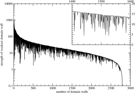
Figure 5: Bottom-up segmentation history for E. coli K-12 MG1655 derived from the initial $(K=0,n=1000)$ paired sliding windows segmentation containing $M=2781$ domain walls. (Inset) Bottom-up segmentation history from $M=1600$ domain walls remaining to $M=1400$ domain walls remaining, showing the fine structure of dips below the smooth envelope.

Like recursive segmentation, there are many detail variations on the implementation of such a coarse graining scheme. The first thing we do is to select a cutoff strength $\Delta^{*}$, which we can think of as a knob we tune to get a desired granularity for our description of the genome: we keep a large number of domain walls if $\Delta^{*}$ is small, and keep a small number of domain walls if $\Delta^{*}$ is large. After selecting $\Delta^{*}$, we can then remove all domain walls weaker than $\Delta^{*}$ in one fell swoop, or remove them progressively, starting from the weakest domain walls. However we decide to remove domain walls weaker than $\Delta^{*}$, the strengths of the remaining domain walls must be re-evaluated after some have been removed from the segmentation. This is done by re-estimating the maximum-likelihood transition probabilities, and using them to compute the Jensen-Shannon divergences between successive coarse-grained segments, which are the strengths of our remaining domain walls. For the purpose of benchmarking, we start from the $(K=0,n=1000)$ paired sliding windows segmentation containing $M=2781$ domain walls for the E. coli K-12 MG1655 genome, and remove the weakest domain wall each time to generate a bottom-up segmentation history, shown in Fig. 5. As we can see, the strength of the weakest domain wall as a function of the number of domain wall remaining consists of a smooth envelope, and dips below this envelope. We distinguish between sharp dips, which are the signatures of what we called tunneling events, and broad dips, which are the signatures of what we called cascade events.

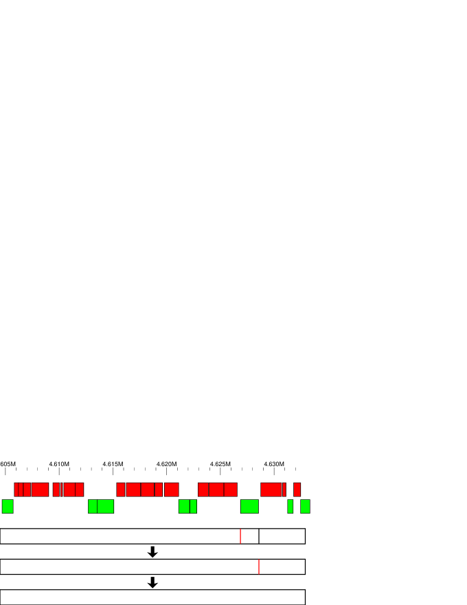
Figure 6: A tunneling event occuring between $M=1586$ and $M=1584$ domain walls remaining in the bottom-up segmentation history of E. coli K-12 MG1655 ($N=4639675$ bp), starting from the $(K=0,n=1000)$ initial segmentation containing $M=2791$ domain walls. Three segments in the $(4604497,4632896)$ region of the genome are shown. The short segment involved in this tunneling event consists of the single gene yjjX on the negative strand (green), flanked by two segments consisting of genes found predominantly on the positive strand (red). At each stage of the bottom-up segmentation history, the domain wall removed is highlighted in red.

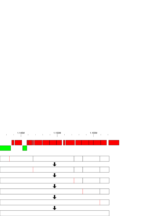
Figure 7: A cascade event occuring between $M=1846$ and $M=1841$ domain walls remaining in the bottom-up segmentation history of E. coli K-12 MG1655 ($N=4639675$ bp), starting from the $(K=0,n=1000)$ initial segmentation containing $M=2791$ domain walls. Six segments in the $(1142115,1157158)$ region of the genome are shown. The first domain wall to be removed in this cascade event lies close to the boundary between the gene rne, believed to be RNase E, on the negative strand (green), and the gene yceQ, coding for a hypothetical protein, on the positive strand (red). The second domain wall to be removed in the cascade is in the middle of the gene rpmF on the positive strand, the third is close to the boundary between fabF and pabC, the fourth is close to the boundary between pabC and yceG, and the last is close to the boundary between holB and ycfH. At each stage of the bottom-up segmentation history, the domain wall removed is highlighted in red.

Looking more closely at the segment statistics, we realized that a tunneling event involves a short segment flanked by two long segments which are statistically similar to one another, but different from the short segment. This statistical dissimilarity between the short segment and its long flanking segments is reflected in the moderate strengths $\Delta_{L}$ and $\Delta_{R}$ of the left and right domain walls of the short segment. Let us say the right domain wall is slightly weaker than the left domain wall, i.e. $\Delta_{R}\lesssim\Delta_{L}$. As the bottom-up segmentation history progresses, there will reach a stage where we remove the right domain wall. When this happens, the short segment will be assimilated by its right flanking segment. Because the right flanking segment is long, absorbing the short segment represents only a small perturbation in its segment statistics. The longer right segment that results is still statistically similar to the left segment. Therefore, when we recompute the strength $\Delta_{L}$ of the remaining domain wall, we find that it is now smaller than the strength $\Delta_{R}$ of the domain wall that was just removed. This remaining domain wall therefore becomes the next to be removed in the bottom-up segmentation history, afterwhich the next domain wall to be removed occurs somewhere else in the sequence, and has strength slightly larger than $\Delta_{R}$. The signature of a tunneling event is therefore a sharp dip in the bottom-up segmentation history. Biologically, a short segment with a tunneling event signature is likely to represent an insertion sometime in the evolutionary past of the organism. A tunneling event in the $(K=0,n=1000)$ bottom-up segmentation history is shown in Fig. 6. In contrast, a cascade event involves a cluster of short segments of varying statistics flanked by two long segments that are statistically similar. The domain walls separating the short segments from each other and from the long flanking segments are then removed in succession. This sequential removal of domain walls gives rise to an extended dip in the bottom-up segmentation history, with a complex internal structure that depends on the actual distribution of short segments. Biologically, a cluster of short segments participating in a cascade event points to a possible recombination hotspot on the genome of the organism. A cascade event in the $(K=0,n=1000)$ bottom-up segmentation history is shown in Fig. 7.

Clearly, by removing more and more domain walls, we construct a proper hierarchy of segmentations containing fewer and fewer domain walls, which agrees intuitively with our notion of what coarse graining is about. We also expected to obtain a unique coarse-grained segmentation, containing only domain walls stronger than $\Delta^{*}$, by removing all domain walls weaker than $\Delta^{*}$. It turned out the picture that emerge from this coarse graining procedure is more complicated, based on which we identified three main problems. First, let us start with a segmentation containing domain walls weaker than $\Delta^{*}$, and decide to remove these domain walls in a single step. Recomputing the strengths of the remaining domain walls, we would find that some of these will be weaker than $\Delta^{*}$, and so cannot claim to have found the desired coarse-grained segmentation. Naturally, we iterate the process, removing all domain walls weaker than $\Delta^{*}$, and recomputing the strengths of the remaining domain walls, until all remaining domain walls are stronger than $\Delta^{*}$. Next, we try removing domain walls weaker than $\Delta^{*}$ one at a time, starting from the weakest, and recompute domain wall strengths after every removal. The strengths of a few of the remaining domain walls will change each time the weakest domain wall is removed, sometimes becoming stronger, and sometimes becoming weaker, but we continue removing the weakest domain wall until all remaining domain walls are stronger than $\Delta^{*}$. Comparing the segmentations obtained using the two coarse-graining procedures, we will find that they can be very different. This difficulty occurs for all averaging problems, so we are not overly concerned, but argue instead that removing the weakest domain wall each time is like a renormalization-group procedure, and should therefore be more reliable than removing many weak domain walls all at once.

Once we accept this decremental procedure for coarse graining, we arrive at the second problem. Suppose we do not stop coarse graining after arriving at the first segmentation with all domain walls stronger than $\Delta^{*}$, but switch strategy to target and removing segments associated with tunneling and cascade events. The segmentations obtained after all domain walls associated with such segments will contain only domain walls stronger than $\Delta^{*}$, but the segmentations in the intermediate steps will contain domain walls weaker than $\Delta^{*}$. If we keep coarse graining until no tunneling or cascade events weaken domain walls below $\Delta^{*}$, we would end up with a series of coarse-grained segmentations containing different number of domain walls. These segmentations do not have the same minimum domain wall strengths, but are related to each other through stages in which some domain walls are weaker than $\Delta^{*}$. We worry about this series of segmentations when there exist domain walls with equal or nearly equal strengths. If at any stage of the coarse graining, these domain walls become the weakest overall, and we stick to removing one domain wall at a time, we can remove any one of these equally weak domain walls. If we track the different bottom-up segmentation histories associated with each choice, we will find that the coarse-grained segmentations for which all domain walls first become stronger than $\Delta^{*}$ can be very different. However, if we coarse grain further by targetting tunneling and cascading segments, we would end up with the same coarse-grained segmentation for which no domain walls ever become weaker than $\Delta^{*}$. Another way to think of this coarsest segmentation is that it is the one for which no domain wall stronger than $\Delta^{*}$ can be added without first adding a domain wall weaker than $\Delta^{*}$.

Third, we know from the bottom-up segmentation history that short segments participating in tunneling events can be absorbed into their long flanking segments without appreciably changing the strengths of the latter’s other domain walls. Clearly, absorbing statistically very distinct short segments increases the heterogenuity of the coarse-grained segment. This is something we have to accept in coarse graining, but ultimately, what we really want at each stage of the coarse graining is for segments to be no more heterogeneous than some prescribed segment variance. Unfortunately, the segment variances are not related to the domain wall strengths in a simple fashion, and even if we know how to compute these segment variances, there is no guarantee that a coarse graining scheme based on these will be less problematic. The bottomline is, all these problems arise because domain wall strengths change wildly as segments are agglomerated in the coarse graining process, due again to the context sensitivity of the Jensen-Shannon divergence (or any other entropic measure, for that matter).

III Mean-Field Analyses of Segmentation Schemes

From our segmentation and coarse graining analyses of real genomes in Sec. II, we realized that these cannot be thought of as consisting of long segments that are strongly dissimilar to its neighboring long segments, within which we find short segments that are weakly dissimilar to its neighboring short segments. In fact, the results suggest that there are short segments that are strongly dissimilar to its neighboring long segments, which are frequently only weakly dissimilar to its neighboring long segments. This mosaic and non-hierarchical structure of segments is the root of the context sensitivity problem, which we will seek to better understand in this section.

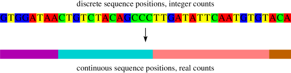
Figure 8: Going from a discrete description to a continuum description of a nucleotide sequence.

To do this, we go first to a continuum description of discrete genomic sequences, as shown in Fig. 8, where we allow the sequence positions and the various $K$-mer frequencies to vary continuously. To eliminate spatial inhomogenuities in the statistics of the interval $[i,j>i)$, which we want to model as a statistically stationary segment in the mean-field limit, we distribute its $K$-mer statistics uniformly along the segment. More precisely, if $f_{\mathbf{t}s}^{[i,j)}$ is the number of times the $(K+1)$-mer $\alpha_{t_{K}}\cdots\alpha_{t_{1}}\alpha_{s}$, which we also refer to as the transition $\mathbf{t}\to s$, appears in $[i,j)$, we define the mean-field count $f_{\mathbf{t}s}^{[i^{\prime},j^{\prime})}$ of the transition $\mathbf{t}\to s$ within the subinterval $[i^{\prime},j^{\prime}>i^{\prime})\subseteq[i,j)$ to be

$$f_{\mathbf{t}s}^{[i^{\prime},j^{\prime})}\equiv\frac{j^{\prime}-i^{\prime}}{j-i}\,f_{\mathbf{t}s}^{[i,j)}.$$ (1)

Within this mean-field picture, we discuss in Sec. III-A how the paired sliding-window scheme’s ability to detect domain walls depends on the size $n$ of the pair of sliding windows. We show, in contrast to the positions and strengths being determined exactly by this segmentation scheme for domain walls between segments both longer than $n$, that domain walls between segments, one or both of which are shorter than $n$, are weakened and shifted in the mean-field limit. Following this, we show in Sec. III-B that the strengths of the domain walls obtained from the recursive segmentation scheme are context sensitive, and approach the exact strengths only as we approach the terminal segmentation. We explain why optimization is desirable at every step of the recursive segmentation, before going on to explain why repetitive sequences are the worst kind of sequences to segment in Sec. III-C. In this section, we present numerical examples for $K=0$ Markov chains, but all qualitative conclusions are valid for Markov chains of order $K>0$.

III-A Paired Sliding Windows Segmentation Scheme

For a pair of windows of length $n$ sliding across a mean-field sequence, there are three possibilities (see Fig. 9):

1. both windows lie entirely within a single mean-field segment;

2. the two windows straddle two mean-field segments, i.e. a single domain wall within one of the windows;

3. the two windows straddle multiple mean-field segments.

The first situation is trivial, as the left and right windowed counts are identical,

$$f_{\mathbf{t}s}^{L}=f_{\mathbf{t}s}^{R}=\frac{n}{N_{\text{seg}}}\,f_{\mathbf{t}s}^{\text{seg}},$$ (2)

$N_{\text{seg}}$ being the length of the mean-field segment, and $f_{\mathbf{t}s}^{\text{seg}}$ being the transition counts within the mean-field segment. The Jensen-Shannon divergence, or the square deviation between the two windows therefore vanishes identically. The second situation, which is what the paired sliding windows segmentation scheme is designed to handle, is analyzed in App. -B4. Based on that analysis, we showed that the position and strength of the domain wall between the two mean-field segments can be determined exactly. We also derived the mean-field lineshape for match filtering.

Figure 9: The three possible situations that we encounter when we slide a symmetric pair of windows across a sequence composed of many mean-field segments: (1) both windows lie entirely within a single mean-field segment; (2) the two windows straddle two mean-field segments; and (3) the two windows straddle multiple mean-field segments.

In this subsection, our interest is in understanding how the paired sliding windows segmentation scheme behaves in the third situation. Clearly, the precise structure of the mean-field divergence spectrum will depend on the local context the pair of windows is sliding across, so we look at an important special case: that of a pair of length-$n$ windows sliding across a segment shorter than $n$. In Fig. 10, we show two lineshapes which are expected to be generic, for (i) the long segments flanking the short segment are themselves statistically dissimilar (top plot); and (ii) the long segments flanking the short segment are themselves statistically similar (bottom plot). In case (i), the mean-field lineshape obtained as the pair of windows slides across the short segment consists of a single peak at one of its ends. This peak is broader than that of a simple domain wall by the width of the short segment, and therefore, if we perform match filtering using the quadratic mean-field lineshape in Eq. (17), the center of the match-filtered peak would occur not at either ends of the short segment, but somewhere in the interior.

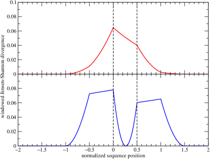
Figure 10: The Jensen-Shannon divergence $\Delta(z)$ (solid curves) of a pair of sliding windows of length $n=1$ as it slides across the binary mean-field segments (left to right) $a$, $b$, and $c$, with lengths $N_{a}>1$, $N_{b}<1$, and $N_{c}>1$ respectively. On the above plots, the left and right ends of segment $b$ are highlighted by the dashed vertical lines at the normalized sequence positions $z=0$ and $z=0.5$ respectively. For the top plot, the probabilities associated with the mean-field segments are $P_{a}(0)=1-P_{a}(1)=0.30$, $P_{b}(0)=1-P_{b}(1)=0.50$, and $P_{c}(0)=1-P_{c}(1)=0.60$. For the bottom plot, the probabilities associated with the mean-field segments are $P_{a}(0)=1-P_{a}(1)=0.20$, $P_{b}(0)=1-P_{b}(1)=0.70$, and $P_{c}(0)=1-P_{c}(1)=0.22$.

In case (ii), the mean-field lineshape obtained as the pair of windows slides across the short segment consists of a pair of peaks, both of which are narrower than the mean-field lineshape of a single domain wall. After we perform match filtering, the center of the match-filtered left peak would be left of the true left domain wall, while the center of the match-filtered right peak would be right of the true right domain wall. Case (ii) is of special interest to us, as it is the context that give rise to tunneling events in the bottom-up segmentation history. Both contexts give rise to shifts in the domain wall positions, as well as to changes in the strengths of the unresolved domain walls, and thus may be able to explain some of the observations made in Sec. II-A. In case (i), the domain wall strength can increase or decrease, depending on how different the two long flanking segments are compared to the short segment. In case (ii), the domain wall strengths always decrease.

III-B Optimized Recursive Jensen-Shannon Segmentation Scheme

To understand how the optimized recursive Jensen-Shannon segmentation is sensitive to global context, let us first understand what happens when the segments discovered recursively are not optimized, and then consider the effects of segmentation optimization. In Fig. 11, we show the Jensen-Shannon divergence spectrum for a sequence consisting of ten mean-field segments. As we can see, the mean-field Jensen-Shannon divergence is everywhere convex, except at the domain walls. These are associated with peaks or kinks in the divergence spectrum, depending on the global context within the sequence. Under special distributions of the segment statistics, domain walls may even have vanishing divergences.

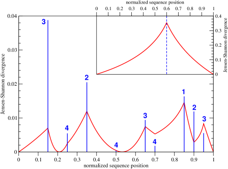
Figure 11: The Jensen-Shannon divergence $\Delta(z)$ (red solid curve) as a function of the normalized cursor position $z$ within an artificial binary sequence composed of ten mean-field segments, characterized by the probabilities (left to right) $\mathbf{P}(0)=(0.55,0.05,0.20,0.60,0.65,0.30,0.45,0.05,0.45,0.15)$. The blue bars indicate the true strengths of each of the nine domain walls, at $z_{1}=0.15$, $z_{2}=0.25$, $z_{3}=0.35$, $z_{4}=0.50$, $z_{5}=0.65$, $z_{6}=0.70$, $z_{7}=0.85$, $z_{8}=0.90$, and $z_{9}=0.95$, while the number at each domain wall indicate which recursion step it is discovered. (Inset) The Jensen-Shannon divergence $\Delta(z)$ (red solid curve) as a function of the normalized cursor position $z$ within an artificial binary sequence composed of two mean-field segments, characterized by the probabilities $P_{L}(0)=0.10$ and $P_{R}(0)=0.90$. The domain wall at $z=0.60$ is indicated by the blue dashed vertical line.

All nine domain walls in the ten-segment sequence are recovered if we allow the recursive Jensen-Shannon segmentation without segmentation optimization to go to completion. However, as shown in Fig. 11, these domain walls are not discovered in the order of their true strengths (heights of the blue bars), given by the Jensen-Shannon divergence between the pairs of segments they separate. In fact, just like in the coarse graining procedure described in Sec. II-C, the Jensen-Shannon divergence at each domain wall changes as the recursion proceeds, as the context it is found in gets refined. For this ten-segment sequence, the recursive segmentation scheme’s sensitivity to global context results in the third strongest domain wall being discovered in the first recursion step, the second and fourth strongest domain walls being discovered in the second recursion step, and the strongest domain wall being discovered only in the third recursion step.

To see the extent to which optimization ameliorate the global context sensitivity of the recursive segmentation scheme, let us imagine the ten-segment sequence to be part of a longer sequence being recursively segmented. Let us further suppose that under segmentation optimization, the segment $(0.95,1.00)$ gets incorporated by the sequence to the right of $(0.00,1.00)$. With this, we now examine in detail a nine-segment sequence $(0.00,0.95)$, whose mean-field divergence spectrum is shown in Fig. 12, instead of the original ten-segment sequence $(0.00,1.00)$. From Fig. 12, we find the divergence maximum of the nine-segment sequence is at $z_{3}=0.35$, the second strongest of the nine domain walls, instead of the third strongest domain wall at $z_{7}=0.85$ for the ten-segment sequence. In proportion to the length of the ten-segment sequence, this shift from the third strongest domain wall to the second strongest domain wall is huge, by about half the length of the sequence, when the change in context involves a loss of only 5% of the total length. In Sec. II-B, we saw instances of such large shifts in optimized domain wall positions when we recursively add one new domain wall each time to a real genome.

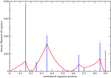
Figure 12: The windowless Jensen-Shannon divergence spectrum $\Delta(z)$ (red solid curve) of the nine-segment binary sequence, after losing the short segment at its right end. The blue bars indicate the strength of each of the nine domain walls.

In this example of the ten-segment sequence, we saw that segmentation optimization has the potential to move an existing domain wall, from a weaker (the third strongest overall), to a stronger (the second strongest overall, and if the global context is different, perhaps even to the strongest overall) position. However, the nature of the context sensitivity problem is such that no guarantee can be offered on the segmentation optimization algorithm always moving a domain wall from a weaker to a stronger position. Nevertheless, segmentation optimization frequently does move a domain wall from a weaker position to a stronger position, and it always make successive segments as statistically distinct from each other as possible. This is good enough a reason to justify the use of segmentation optimization.

III-C Repetitive Sequences

In this last subsection of Sec. III, let us look at repetitive sequences, for which the context sensitivity problem is the most severe. Such sequences, which are composed of periodically repeating motifs, are of biological interest because they arise from a variety of recombination processes, and are fairly common in real genomic sequences. In general, a motif $a_{1}a_{2}\cdots a_{r}$ that is repeated in a repetitive sequence can consists of $r$ statistically distinct subunits, but for simplicity, let us look only at $ab$-repeats, and highlight statistical signatures common to all repetitive sequences.

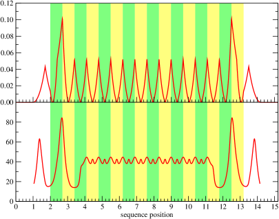
Figure 13: The Jensen-Shannon divergence spectrum (top, red solid curve) before, and (bottom, red solid curve) after match filtering and quality enhancement, for a pair of windows of size $n=1$ sliding across a repetitive binary $K=0$ sequence $cababababababababc$, where the subunits $a$ (light green) and $b$ (light yellow) both have lengths $n_{a}=n_{b}=0.7$, and are characterized by the probabilities $P_{a}(0)=1-P_{a}(1)=0.1$ and $P_{b}(0)=1-P_{b}(1)=0.9$. The terminal $c$ segments (white), assumed to have lengths much larger than $n=1$, are characterized by the probability $P_{c}(0)=1-P_{c}(1)=0.5$.

When we segment the repetitive sequence $abababababababab$ using the paired sliding windows segmentation scheme with window size $n$, we obtained the mean-field Jensen-Shannon divergence spectrum shown in the top plot of Fig. 13. In this figure, sequence positions are normalized such that $n=1$, while the lengths of the repeating segments $a$ and $b$ are chosen to be both less than the window size, i.e. $n_{a}=n_{b}=0.7<n$. To understand contextual effects at the ends of the repetitive sequence, we include the terminal segments $c$ in our analysis. These terminal $c$ segments are assumed to have lengths $n_{c}\gg n$, and statistics intermediate between those of $a$ and $b$. As we can see from the top plot of Fig. 13, all domain walls between $a$ and $b$ segments ($ab$ domain walls) correspond to peaks in the mean-field divergence spectrum. The two $ab$ domain walls near the ends of the repetitive sequence are the strongest, while the rest have the same diminished strength (compared to the Jensen-Shannon divergence between the $a$ and $b$ segments). From the top plot of Fig. 13, we also see that no peaks are associated with the $ca$ and $bc$ domain walls. Instead, we find a spurious peak left of the $ca$ domain wall, and another spurious peak right of the $bc$ domain wall.

As discussed in App. -B, the mean-field lineshape of a simple domain wall is very nearly piecewise quadratic, with a total width of $2n$. This observation is extremely helpful when we deal with real divergence spectra, where statistical fluctuations produce spurious peaks with various shapes and widths. By insisting that only peaks that are (i) approximately piecewise quadratic, with (ii) widths close to $2n$, are statistically significant, we can determine a smaller, and more reliable set of domain walls through match filtering. In the top plot of Fig. 13, all our peaks have widths smaller than $2n$. In the mean-field limit, these are certainly not spurious, but if we imagine putting statistical fluctuations back into the divergence spectrum, and suppose we did not know beforehand that there are segments shorter than $n$ in this sequence, it would be reasonable to accept by fiat whatever picture emerging from the match filtering procedure. For $cababababababababc$, the match-filtered, quality enhanced divergence spectrum is shown as the bottom plot of Fig. 13, where we find the two spurious peaks shifted deeper into the $c$ segments by the match filtering procedure. In this plot, the two strong $ab$ domain walls near the ends of the repetitive sequence continue to stand out, but the rest of the $ab$ domain walls are now washed out by match filtering. If we put statistical noise back into the picture, the fine structures marking these remaining $ab$ domain walls will disappear, and we end up with a featureless plateau in the interior of the repetitive sequence. We might then be misled into thinking that this $cababababababababc$ sequence consists of only five segments $ca^{\prime}c^{\prime}b^{\prime}c$, where $a^{\prime}$ is $a$ contaminated by a small piece of $c$, $b^{\prime}$ is $b$ contaminated by a small piece of $c$, and $c^{\prime}$, which lies between the two strong $ab$ domain walls, will be mistaken for a segment with $K=0$ statistics similar to $c$, even though it is not statistically stationary.

Next, let us analyze the recursive Jensen-Shannon segmentation of $abababababababab$, where we cut the repetitive sequence first into two segments, then each of these into two subsegments, and so on and so forth, until all the segments are discovered. In the top plot of Fig. 14, we show the top-level Jensen-Shannon divergence spectrum, based on which we will cut $abababababababab$ into two segments. In this figure, we find

1. a series of $k$ peaks of unequal strengths, with stronger peaks near the ends, and weaker peaks in the middle of the repetitive sequence;

2. $k-1$ domain walls having vanishing divergences;

3. the ratio of strengths of the strongest peak to the weakest peak is roughly $k/2$,

where $k$ is the number of repeated motifs. These statistical signatures are shared by all repetitive sequences, with the detail distribution and statistical characteristics of the subunits within the repeated motif affecting only the shape and strength of the peaks. Here we see extreme context sensitivity reflected in the fact that domain walls with the same true strength can have very different, and even vanishing, strengths when the segment structure of the sequence is examined recursively.

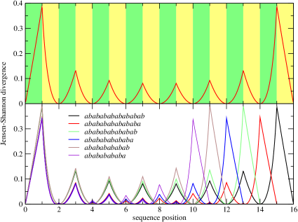
Figure 14: (Top) The top-level Jensen-Shannon divergence spectrum (red solid curve) obtained in the recursive segmentation of a repetitive binary sequence consisting of subunits $a$ (light green, $P_{a}(0)=1-P_{a}(1)=0.1$) and $b$ (light yellow, $P_{b}(0)=1-P_{b}(1)=0.9$) repeated eight times. (Bottom) The Jensen-Shannon divergence spectra obtained when $abababababababab$ is recursively segmented from the right end.

From the bottom plot of Fig. 14, we find that one or both of the peaks near the ends of the repetitive sequence are always the strongest, as recursion progresses. This is true when the repetitive sequence consists of repeating motifs with more complex internal structure, and also true when we attach terminal segments to the repetitive sequence. Therefore, successive cuts are always made at one end or the other of the repetitive sequence. For $ab$-repeats, the peaks near both ends are equally strong in the mean-field limit, so we can choose to always cut at the right end of $abababababababab$, as shown in the bottom plot of Fig. 14. As the repetitive sequence loses its rightmost segment at every step, and the global context alternates between being dominated by $a$ segments to being dominated by $b$ segments, we find oscillations in the strengths of the remaining domain walls. This oscillation, which is a generic behaviour of all repetitive sequences under recursive segmentation, can be seen more clearly for the $ab$-repetitive sequence in Figure 15, where instead of cutting off one segment at a time, we move the cut continuously inwards from the right end.

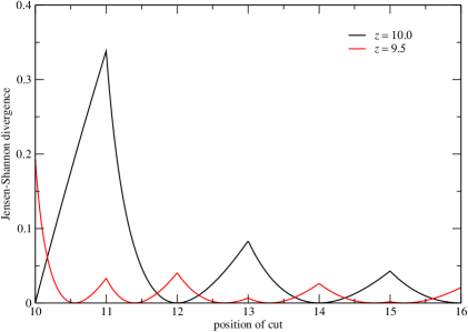
Figure 15: The windowless Jensen-Shannon divergences at $z=10.0$ (at a domain wall) and $z=9.5$ (away from a domain wall) of the repetitive binary sequence $abababababababab$, with $P_{a}(0)=0.1$ and $P_{b}(0)=0.9$, as functions of the cut $10\leq z\leq 16$.

IV Summary and Discussions

In this paper, we defined the context sensitivity problem, in which the same group of statistically stationary segments are segmented differently by the same segmentation scheme, when it is encapsulated within different larger contexts of segments. We then described in Sec. II the various manifestions of context sensitivity when real bacterial genomes are segmented using the paired sliding windows and optimized recursive Jensen-Shannon segmentation schemes, which are sensitive to local and global contexts respectively. For the single-pass paired sliding windows segmentation scheme, we found that the positions and relative strengths of domain walls can change dramatically when we change the window size, and hence the local contexts examined. For the optimized recursive segmentation scheme, we found that there can be large shifts in the optimized domain wall positions as recursion progresses, due to the change in global context when we go from examining a sequence to examining its subsequence, and vice versa.

In Sec. II, we also looked into the issue of coarse graining the segmental description of a bacterial genome. We argued that coarse graining by using larger window sizes, or stopping recursive segmentation earlier can be biologically misleading, because of the context sensitivity problem, and explored an alternative coarse graining procedure which involves removing the weakest domain walls and agglomerating the segments they separate. This coarse graining procedure was found to be fraught with difficulties, arising again from the context sensitivity of domain wall strengths. Ultimately, the goal of coarse graining is to reduce the complexity of the segmented models of real genomes. This can be achieved by reducing the number of segments, or by reducing the number of segment types or classes (see, for example, the work by Azad et al. [4]). We realized in this paper that the former is unattainable, and proposed to accomplish the latter through statistical clustering of the segments. Based on what we understand about the context sensitivity problem, we realized that it would be necessary to segment a given genomic sequence as far as possible, to the point before genes are cut into multiple segments (unless they are known to contain multiple domains). We are in the process of writing the results of our investigations into this manner of coarse graining, in which no domain walls are removed, but statistically similar segments are clustered into a small number of segment classes.

In Sec. III, we analyzed the paired sliding windows and optimized recursive segmentation schemes within a mean-field picture. For the former, we explained how the presence of segments shorter than the window size lead to shifts in the positions, and changes in the strengths of domain walls. For the latter, we illustrate the context dependence of the domain walls strengths, how this leads to large shifts in the optimized domain wall positions, and also to the domain walls being discovered out of order by their true strengths. We showed that all domain walls in a sequence will be recovered in the mean-field limit, if we allow the recursive segmentation to go to completion, but realized that for real sequences subject to statistical fluctuations, there is a danger of stopping the the recursion too early. When this happens, we will generically pick up weak domain walls, but miss stronger ones — a problem that can be partly alleviated through segmentation optimization, in which domain walls are moved from weaker to stronger positions. We devoted one subsection to explain why the context sensitivity problem is especially severe in repetitive sequences.

Finally, let us say that while we have examined only two entropic segmentation schemes in detail, we believe the context sensitivity problem plagues all segmentation schemes. The manifestations of the context sensitivity problem will of course be different for different segmentation schemes, but will involve (i) getting the domain wall positions wrong; (ii) getting the domain wall strengths wrong; or (iii) missing strong domain walls. A proper analysis of the context sensitivity of the various segmentation schemes is beyond the scope of this paper, but let us offer some thoughts on segmentation schemes based on based on hidden Markov models (HMMs), which are very popular in the bioinformatics literature. In HMM segmentation, model parameters are typically estimated using the Baum-Welch algorithm, which first computes the forward and backward probabilities of each hidden state, use these to estimate the transition frequencies, which are used to update the model parameters. Computation of forward and backward probabilities are sensitive to local context, in that the hidden states assigned to a given collection of segments will be different, if the sequences immediately flanking the segments are different. Updating of model parameters, on the other hand, is sensitive to global context, because very different arrangement of segments and segment classes can give rise to the same summary of transition frequencies. The signatures of this dual local-global context sensitivity is buried within the sequence of posterior probabilities obtained from iterations of the Baum-Welch algorithm. Ultimately, the context sensitivity problem is a very special case of the problem of mixed data, which is an active area of statistical research. We hope that through the results presented in this paper, the bioinformatics community will come to better recognize the nuances sequence context poses to its proper segmentation.

-A Generalized Jensen-Shannon Divergences

In Ref. 2 we explained that dinucleotide correlations and codon biases in biological sequences [5, 6, 7, 8, 9] are better modeled by Markov chains of order $K>0$ over the quaternary alphabet $\mathcal{S}=\rm\{A,C,G,T\}$ [10], rather than Bernoulli chains over $\mathcal{S}$ [11, 12], or Bernoulli chains over the extended alphabet $\mathcal{S}^{K}$ [13, 14, 15]. In the sequence segmentation problem, our task is to decide whether there is a domain wall at sequence position $i$ within a given sequence $\mathbf{x}=x_{1}x_{2}\cdots x_{i-1}x_{i}x_{i+1}\cdots x_{N}$, where $x_{j}\in\mathcal{S},1\geq j\geq N$. The simplest model selection scheme that would address this problem would involve the comparison of the one-segment sequence likelihood $P_{1}$, whereby the sequence $\mathbf{x}$ is treated as generated by a single Markov process, against the two-segment sequence likelihood $P_{2}$, whereby the subsequences $\mathbf{x}_{L}=x_{1}x_{2}\cdots x_{i-1}$ and $\mathbf{x}_{R}=x_{i}x_{i+1}\cdots x_{N}$ are treated as generated by two different Markov processes.

To model $\mathbf{x}$, $\mathbf{x}_{L}$, and $\mathbf{x}_{R}$ as Markov chains of order $K$, we determine the order-$K$ transition counts $f_{\mathbf{t}s}$, $f_{\mathbf{t}s}^{L}$, $f_{\mathbf{t}s}^{R}$, subject to the normalizations

$$f_{\mathbf{t}s}=f_{\mathbf{t}s}^{L}+f_{\mathbf{t}s}^{R},\quad\sum_{\mathbf{t}\in\mathcal{S}^{K}}\sum_{s=1}^{S}f_{\mathbf{t}s}=N.$$ (3)

Here $S=4$ is the size of the quaternary alphabet $\mathcal{S}$, and $\mathbf{t}$ is a shorthand notation for the $K$-tuple of indices $(t_{1},t_{2},\dots,t_{K}),1\leq t_{k}\leq S$. The transition counts $f_{\mathbf{t}s}$, $f_{\mathbf{t}s}^{L}$, and $f_{\mathbf{t}s}^{R}$ are the number of times the $(K+1)$-mer $\alpha_{t_{K}}\cdots\alpha_{t_{1}}\alpha_{s}$ appear in the sequences $\mathbf{x}$, $\mathbf{x}_{L}$, and $\mathbf{x}_{R}$ respectively. The sequences $\mathbf{x}$, $\mathbf{x}_{L}$, and $\mathbf{x}_{R}$ are then assumed to be generated by the Markov processes with maximum-likelihood transition probabilities

$$\hat{p}_{\mathbf{t}s}=\frac{f_{\mathbf{t}s}}{\sum_{s^{\prime}=1}^{S}f_{\mathbf{t}s^{\prime}}},\quad\hat{p}_{\mathbf{t}s}^{L}=\frac{f_{\mathbf{t}s}^{L}}{\sum_{s^{\prime}=1}^{S}f_{\mathbf{t}s^{\prime}}^{L}},\quad\hat{p}_{\mathbf{t}s}^{R}=\frac{f_{\mathbf{t}s}^{R}}{\sum_{s^{\prime}=1}^{S}f_{\mathbf{t}s^{\prime}}^{R}},$$ (4)

respectively.

Within these maximum-likelihood Markov-chain models, the one- and two-segment sequence likelihoods are given by

$$P_{1} =\prod_{\mathbf{t}\in\mathcal{S}^{K}}\prod_{s=1}^{S}\left(\hat{p}_{\mathbf{t}s}\right)^{f_{\mathbf{t}s}},$$ (5)

$$P_{2} =\prod_{\mathbf{t}\in\mathcal{S}^{K}}\prod_{s=1}^{S}\left(\hat{p}_{\mathbf{t}s}^{L}\right)^{f_{\mathbf{t}s}^{L}}\left(\hat{p}_{\mathbf{t}s}^{R}\right)^{f_{\mathbf{t}s}^{R}},$$

respectively. Because we have more free parameters to fit the observed sequence statistics in the two-segment model, $P_{2}\geq P_{1}$. The generalized Jensen-Shannon divergence, a symmetric variant of the relative entropy known more commonly as the Kullback-Leibler divergence, is then given by

$$\Delta(i)=\log\frac{P_{2}}{P_{1}}=\sum_{\mathbf{t}\in\mathcal{S}^{K}}\sum_{s=1}^{S}\left[-f_{\mathbf{t}s}\log\hat{p}_{\mathbf{t}s}+f_{\mathbf{t}s}^{L}\log\hat{p}_{\mathbf{t}s}^{L}+f_{\mathbf{t}s}^{R}\log\hat{p}_{\mathbf{t}s}^{R}\right].$$ (6)

This test statistic, generalized from the Jensen-Shannon divergence described in Ref. 16, measures quantitatively how much better the two-segment model fits $\mathbf{x}$ compared to the one-segment model.

-B Paired Sliding Windows Segmentation Scheme

A standard criticism on using sliding windows to detect segment structure within a heterogeneous sequence is the compromise between precision and statistical significance. For the comparison between two windowed statistics to be significant, we want the window size $n$ to be large. On the other hand, to be able to determine a change point precisely, we want the window size $n$ to be small. There is therefore no way, with a single window of length $n$, to independently select both a desired statistical significance and desired precision.

In this appendix, we devise a sliding window segmentation scheme in which, instead of one window, we use a pair of adjoining windows, each of length $n$. By comparing the left windowed statistics to the right windowed statistics, a change point is detected at the center of the pair of windows when the two windowed statistics are most different. A given difference between the two windowed statistics becomes more signficant as the window size $n$ is increased. A larger window size also suppresses statistical fluctuations, making it easier to locate the change point. Therefore, increasing the window size $n$ improves both statistical significance and precision, even though they cannot be adjusted independently.

In App. -B1, we describe the proper test statistic to use for change point detection within the model selection framework. Then in App. -B2, we show how a similar test statistic spectrum can be obtained within the hypothesis testing framework. In App. -B3, we show some examples of the scheme being applied to real genomic sequences. In App. -B4, we derived the mean-field lineshape of a domain wall in this paired sliding window segmentation scheme, and use it to perform match filtering.

-B1 Model Selection Within a Pair of Sliding Windows

To detect domain walls between different segments within a heterogeneous sequence, we can slide a pair of adjoining windows each of length $n$ across the sequence, and monitor the left and right windowed statistics at different sequence positions, as shown in Figure 16.

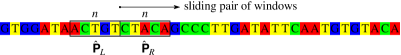
Figure 16: A pair of sliding windows, each of length $n$. A change point at the center of the pair of sliding windows can be detected by comparing the statistics within the left and right windows.

If we model the different segments by Markov chains of order $K$, the left and right windowed statistics are summarized by the transition count matrices

$$\textsf{{F}}^{L}=\left[f_{\mathbf{t}s}^{L}\right],\quad\textsf{{F}}^{R}=\left[f_{\mathbf{t}s}^{R}\right]$$ (7)

respectively, where the transition counts sums to the window size,

$$\sum_{\mathbf{t}}\sum_{s}f_{\mathbf{t}s}^{L}=\sum_{\mathbf{t}}\sum_{s}f_{\mathbf{t}s}^{R}=n.$$ (8)

From these transition count matrices, we can determine the maximum-likelihood estimates

$$\hat{\textsf{{P}}}^{L}=\left[p_{\mathbf{t}s}^{L}\right],\quad p_{\mathbf{t}s}^{L}=\frac{f_{\mathbf{t}s}^{L}}{\sum_{s^{\prime}}f_{\mathbf{t}s^{\prime}}^{L}};\quad\hat{\textsf{{P}}}^{R}=\left[p_{\mathbf{t}s}^{R}\right],\quad p_{\mathbf{t}s}^{R}=\frac{f_{\mathbf{t}s}^{R}}{\sum_{s^{\prime}}f_{\mathbf{t}s^{\prime}}^{R}}$$ (9)

of the transition matrices for the left and right windows.

We then compute the transition count matrix

$$\textsf{{F}}=\left[f_{\mathbf{t}s}=f_{\mathbf{t}s}^{L}+f_{\mathbf{t}s}^{R}\right],$$ (10)

and therefrom the transition matrix

$$\hat{\textsf{{P}}}=\left[p_{\mathbf{t}s}\right],\quad p_{\mathbf{t}s}=\frac{f_{\mathbf{t}s}}{\sum_{s^{\prime}}f_{\mathbf{t}s^{\prime}}},$$ (11)

assuming a one-segment model for the combined window of length $2n$, before calculating the windowed Jensen-Shannon divergence using Eq. (6) in App. -A. By sliding the pair of windows along the sequence, we obtain a windowed Jensen-Shannon divergence spectrum $\Delta(i)$, which tells us where along the sequence the most statistically significant change points are located.

-B2 Hypothesis Testing With a Pair of Sliding Windows

Change point detection using statistics within the pair of sliding windows can also be done within the hypothesis testing framework. Within this framework, we ask how likely it is to find maximum-likelihood estimates $\hat{\textsf{{P}}}^{L}$ for the left window, and $\hat{\textsf{{P}}}^{R}$ for the right window, when the pair of windows straddles a statistically stationary region generated by the transition matrix P.

In the central limit regime, Whittle showed that the probability of obtaining a maximum-likelihood estimate $\hat{\textsf{{P}}}$ from a finite sequence generated by the transition matrix P is given by [17]

$$P(\hat{\textsf{{P}}}|\textsf{{P}})=C\exp\left[\frac{1}{2}\sum_{\mathbf{t}}\sum_{s}\sum_{s^{\prime}}\frac{n}{P_{\mathbf{t}}}\left(1-\frac{\delta_{ss^{\prime}}}{p_{\mathbf{t}s}}\right)\left(\hat{p}_{\mathbf{t}s}-p_{\mathbf{t}s}\right)\left(\hat{p}_{\mathbf{t}s^{\prime}}-p_{\mathbf{t}s^{\prime}}\right)\right],$$ (12)

where $C$ is a normalization constant, $n$ the length of the sequence, and $P_{\mathbf{t}}$ is the equilibrium distribution of $K$-mers in the Markov chain.

For $n\gg K$, the left and right window statistics are essentially independent, and so the probability of finding $\hat{\textsf{{P}}}^{L}$ in the left window and finding $\hat{\textsf{{P}}}^{R}$ in the right window, when the true transition matrix is P, is $P(\hat{\textsf{{P}}}^{L}|\textsf{{P}})P(\hat{\textsf{{P}}}^{R}|\textsf{{P}})$. In principle we do not know what P is, so we replace it by $\hat{\textsf{{P}}}$, the maximum-likelihood transition matrix estimated from the combined statistics in the left and right windows. Based on Eq. (12), the test statistic that we compute as we slide the pair of windows along the sequence is the square deviation

$$r=-\sum_{\mathbf{t}}\sum_{s}\sum_{s^{\prime}}\frac{n}{\hat{P}_{\mathbf{t}}}\left(1-\frac{\delta_{ss^{\prime}}}{\hat{p}_{\mathbf{t}s}}\right)\left[\left(\hat{p}_{\mathbf{t}s}^{L}-\hat{p}_{\mathbf{t}s}\right)\left(\hat{p}_{\mathbf{t}s^{\prime}}^{L}-\hat{p}_{\mathbf{t}s^{\prime}}\right)+\left(\hat{p}_{\mathbf{t}s}^{R}-\hat{p}_{\mathbf{t}s}\right)\left(\hat{p}_{\mathbf{t}s^{\prime}}^{R}-\hat{p}_{\mathbf{t}s^{\prime}}\right)\right],$$ (13)

which is more or less the negative logarithm of $P(\hat{\textsf{{P}}}^{L}|\textsf{{P}})P(\hat{\textsf{{P}}}^{R}|\textsf{{P}})$. To compare the square deviation spectrum $r(i)$ obtained for different window sizes, we simply divide $r(i)$ by the window size $n$. From Eq. (13), we find that $r$ receive disproportionate contributions from rare states ($\hat{P}_{\mathbf{t}}$ small) as well as rare transitions ($\hat{p}_{\mathbf{t}s}$ small).

-B3 Application to Real Genomic Sequences

The average length of coding genes in Escherichia coli K-12 MG1655 is 948.9 bp. This sets a ‘natural’ window size to use for our sliding window analysis. In Figure 17, we show the windowed $K=0$ Jensen-Shannon divergence and square deviation spectra for Escherichia coli K-12 MG1655, obtained for a window size of $n=1000$ bp, overlaid onto the distribution of genes. As we can see from the figure, the two spectra are qualitatively very similar, with peak positions that are strongly correlated with gene and operon boundaries [18].

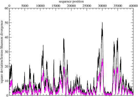
Figure 17: The windowed $K=0$ Jensen-Shannon divergence (magenta) and square deviation (black) spectra in the interval $(0,40000)$ of the Escherichia coli K-12 MG1655 genome, which has a length $N=4639675$ bp. Annotated genes on the positive (red) and negative (green) strands are shown below the graph.

For example, we see that the strongest peak in the $n=1000$ windowed spectrum is at $i\sim 30000$. The gene dapB, believed to be an enzyme involved in lysine (which consists solely of purines) biosynthesis, lies upstream of this peak, while the carAB operon, believed to code for enzymes involved in pyrimidine ribonucleotide biosynthesis, lies downstream of the peak. Another strong peak marks the end of the carAB operon, distinguishing it statistically from the gene caiF, and yet another strong peak distinguishes caiF from the caiTABCDE operon, whose products are involved in the central intermediary metabolic pathways, further downstream.

In Figure 18, we show the square deviation spectra for the same $(0,40000)$ interval of the E. coli K-12 MG1655 genome, but for different Markov-chain orders $K=0,1,2$. As we can see, these square deviation spectra share many qualitative features, but there are also important qualitative differences. For example, the genes talB and mogA, which lies within the interval $(8200,9900)$, are not strongly distinguished from the genes yaaJ upstream and yaaH downstream at the 1-mer ($K=0$) level. They are, however, strongly distinguished from the flanking genes at the 2-mer ($K=1$) and 3-mer ($K=2$) levels.

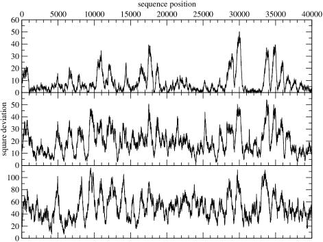
Figure 18: The windowed $K=0$ (top), $K=1$ (middle), and $K=2$ (bottom) square deviation spectra in the interval $(0,40000)$ of the E. coli K-12 MG1655 genome, which has a length of $N=4639675$ bp. Annotated genes on the positive (red) and negative (green) strands are shown below the graph.

-B4 Mean-Field Lineshape and Match Filtering

In the second situation shown in Fig. 9, let us label the two mean-field segments $a$ and $b$, with lengths $N_{a}$ and $N_{b}$. Suppose it is the left window that straddles both $a$ and $b$, while the right window lies entirely within $b$. The right-window counts are then simply

$$f_{\mathbf{t}s}^{R}=\frac{n}{N_{b}}\,f_{\mathbf{t}s}^{b},$$ (14)

while the left-window counts contain contributions from both $a$ and $b$, i.e.

$$f_{\mathbf{t}s}^{L}=\frac{n-z}{N_{a}}\,f_{\mathbf{t}s}^{a}+\frac{z}{N_{b}}\,f_{\mathbf{t}s}^{b},$$ (15)

where $z$ is the distance of the domain wall from the center of the pair of windows. The total counts from both windows are then

$$f_{\mathbf{t}s}=\frac{n-z}{N_{a}}\,f_{\mathbf{t}s}^{a}+\frac{z}{N_{b}}\,f_{\mathbf{t}s}^{b}+\frac{n}{N_{b}}\,f_{\mathbf{t}s}^{b}.$$ (16)

Using the transition counts $f_{\mathbf{t}s}^{L}$, $f_{\mathbf{t}s}^{R}$, and $f_{\mathbf{t}s}$, we then compute the maximum-likelihood transition probabilities $\hat{p}_{\mathbf{t}s}^{L}$, $\hat{p}_{\mathbf{t}s}^{R}$, and $\hat{p}_{\mathbf{t}s}$, before substituting the transition counts and transition probabilities into Eq. (6) for the Jensen-Shannon divergence. Because of the logarithms in the definition for the Jensen-Shannon divergence, we get a complicated function in terms of the observed statistics $f_{\mathbf{t}s}^{a}$, $f_{\mathbf{t}s}^{b}$, $N_{a}$ and $N_{b}$, and the distance $z$ between the domain wall and the center of the pair of windows. Different observed statistics $f_{\mathbf{t}s}^{a}$, $f_{\mathbf{t}s}^{b}$, $N_{a}$ and $N_{b}$ give mean-field divergence functions of $z$ that are not related by a simple scaling. However, these mean-field divergence functions $\Delta(z)$ do have qualitative features in common:

1. $\Delta(z)=0$ for $|z|\geq n$, where the pair of windows is entirely within $a$ or entirely within $b$;

2. $\Delta(z)$ is maximum at $z=0$, when the center of the pair of windows coincide with the domain wall;

3. $\Delta(z)$ is convex everywhere within $|z|<n$, except at $z=0$.

This tells us that the position and strength of the domain wall between two mean-field segments both longer than the window size $n$ can be determined exactly.

In Figure 19 we show $\Delta(z)$ for two binary $K=0$ mean-field segments, where $P_{a}(0)=1-P_{a}(1)=0.9$, and $P_{b}(0)=1-P_{b}(1)=0.1$. We call the peak function $\Delta(z)$ the mean-field lineshape of the domain wall. As we can see from Figure 19, this mean-field lineshape can be very well approximated by the piecewise quadratic function

$$\tilde{\Delta}(z)=\begin{cases}\left(1+\frac{z}{n}\right)^{2}\bar{\Delta}(0),&-1<z<0;\\ \left(1-\frac{z}{n}\right)^{2}\bar{\Delta}(0),&0\leq z<1;\\ 0,&\text{everywhere else},\end{cases}$$ (17)

where $\bar{\Delta}(0)$ is the mean-field Jensen-Shannon divergence of the domain wall at $z=0$. If instead of the windowed Jensen-Shannon divergence $\Delta(z)$, we compute the windowed square deviation $r(z)$ in the vicinity of a domain wall, we will obtain a mean-field lineshape that is strictly piecewise quadratic, i.e.

$$\tilde{r}(z)=\begin{cases}\left(1+\frac{z}{n}\right)^{2}\bar{r}(0),&-1<z<0;\\ \left(1-\frac{z}{n}\right)^{2}\bar{r}(0),&0\leq z<1;\\ 0,&\text{everywhere else},\end{cases}$$ (18)

where $\bar{r}(0)$ is the mean-field square deviation of the domain wall at $z=0$.

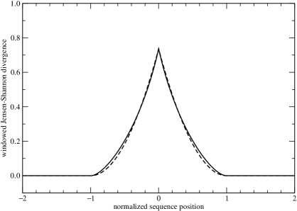
Figure 19: The Jensen-Shannon divergence $\Delta(z)$ (solid curve) of a pair of sliding windows of length $n=1$ as a function of the distance $z$ between the domain wall separating a mean-field binary segment $a$ with $P_{a}(0)=1-P_{a}(1)=0.9$ and a mean-field binary segment $b$ with $P_{b}(0)=1-P_{b}(1)=0.1$, and the center of the pair of windows. Also shown as the dashed curve is a piecewise quadratic function which rises from $z=\pm 1$ to the same maximum at $z=0$, but vanishes everywhere else.

Going back to a real sequence composed of two nearly stationary segments of discrete bases, we expect to find statistical fluctuations masking the mean-field lineshape. But now that we know the mean-field lineshape is piecewise quadratic for the square deviation $r(z)$ (or very nearly so, in the case of the windowed Jensen-Shannon divergence $\Delta(z)$), we can make use of this piecewise quadratic mean-field lineshape to match filter the raw square deviation spectrum. We do this by assuming that there is a mean-field square-deviation peak at each sequence position $i$, fit the spectrum within $(i-n,i+n)$ to the mean-field lineshape in Eq. (18), and determine the smoothed spectrum $\bar{r}(i)$. In Fig. 20, we show the match-filtered square deviation spectrum $\bar{r}(i)$ in the interval $0\leq i\leq 40000$ of the E. coli K-12 MG1655 genome. As we can see, $\bar{r}(i)$ is smoother than $r(i)$, but the peaks in $\bar{r}(i)$ are also so broad that distinct peaks in $r(i)$ are not properly resolved.

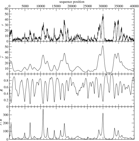
Figure 20: The interval $0\leq i\leq 40000$ of the E. coli K-12 MG1655 genome ($N=4639675$ bp), showing (top to bottom) the windowed $K=0$ square deviation spectrum $r(i)$, the match-filtered square deviation spectrum $\bar{r}(i)$, the residue spectrum $R(i)$, and the quality enhanced square deviation spectrum $\bar{r}(i)/R(i)$. Annotated genes on the positive (red) and negative (green) strands are shown below the graph.

Fortunately, more information is available from the match filtering. We can also compute how well the raw spectrum $r(j)$ in the interval $i-n\leq j\leq i+n$ match the mean-field lineshape $\tilde{r}(j)$ by computing the residue

$$R(i)=\sum_{j=i-n}^{i+n}\left[r(j)-\tilde{r}(j)\right]^{2}.$$ (19)

filtering the raw divergence spectrum. In Fig. 20, we show the residue spectrum $R(i)$ for the $0\leq i\leq 40000$ region of the E. coli K-12 MG1655 genome. In the residue spectrum, we see a series of dips at the positions of peaks in the square deviation spectrum. Since $R(i)$ is small when the match is good, and large when the match is poor, $1/R(i)$ can be thought of as the quality factor of a square deviation peak. A smoothed, and accentuated spectrum is obtained when we divide the smoothed square deviation by the residue at each point. The quality enhanced square deviation spectrum $\bar{r}(i)/R(i)$ is also shown in Fig. 20. It is much more convenient to determine the position of significant domain walls from such a spectrum.

References

- [1] Jerome V. Braun and Hans-Georg Müller, “Statistical Methods for DNA Sequence Segmentation”, Statistical Science 13(2), 142–162 (1998).
- [2] S.-A. Cheong, P. Stodghill, D. J. Schneider, S. W. Cartinhour, and C. R. Myers, “Extending the recursive Jensen-Shannon segmentation of biological sequences”, q-bio/0904.2466.
- [3] V. Joardar, M. Lindeberg, D. J. Schneider, A. Collmer, and C. R. Buell, “Lineage-specific regions in Pseudomonas syringae pv tomato DC3000”, Molecular Plant Pathology 6(1), 53–64 (2005).
- [4] R. K. Azad, J. S. Rao, W. Li, and R. Ramaswamy, “Simplifying the mosaic description of DNA sequences”, Physical Review E 66(3), art. 031913 (2002).
- [5] R. Grantham, C. Gautier, M. Gouy, M. Jacobzone, and R. Mercier, “Codon catalog usage is a genome strategy modulated for gene expressivity”, Nucleic Acids Research 9(1), R43–R74 (1981).
- [6] John C. W. Shepherd, “Method to Determine the Reading Frame of a Protein from the Purine/Pyrimidine Genome Sequence and Its Possible Evolutionary Justification”, Proceedings of the National Academy of Sciences, USA 78(3), 1596–1600 (1981).
- [7] R. Staden and A.D. McLachlan, “Codon preference and its use in identifying protein coding regions in long DNA sequences”, Nucleic Acids Research 10(1), 141–156 (1982).
- [8] James W. Fickett, “Recognition of protein coding regions in DNA sequences”, Nucleic Acids Research 10(17), 5303–5318 (1982).
- [9] Hanspeter Herzel and Ivo Große, “Measuring correlations in symbol sequences”, Physica A 216(4), 518–542 (1995).
- [10] V. Thakur, R. K. Azad, and R. Ramaswamy, “Markov models of genome segmentation”, Physical Review E, vol. 75, no. 1, art. 011915, 2007.
- [11] Pedro Bernaola-Galván, Ramón Román-Roldán, and José L. Oliver, “Compositional segmentation and long-range fractal correlations in DNA sequences”, Physical Review E 53(5), 5181–5189 (1996).
- [12] Ramón Román-Roldán, Pedro Bernaola-Galván, and José L. Oliver, “Sequence Compositional Complexity of DNA through an Entropic Segmentation Method”, Physical Review Letters 80(6), 1344–1347 (1998).
- [13] Pedro Bernaola-Galván, Ivo Grosse, Pedro Carpena, José L. Oliver, Ramón Román-Roldán, and H. Eugene Stanley, “Finding Borders between Coding and Noncoding DNA Regions by an Entropic Segmentation Method”, Physical Review Letters 85(6), 1342–1345 (2000).
- [14] Daniel Nicorici, John A. Berger, Jaakko Astola, and Sanjit K. Mitra, “Finding Borders Between Coding and Noncoding DNA Regions Using Recursive Segmentation and Statistics of Stop Codons”, in Proceedings of the Finnish Signal Processing Symposium (FINSIG ’03, Tampere, Finland, May 2003) edited by Heikki Huttunen, Atanas Gotchev, and Adriana Vasilache, TICSP Series Number 20, 2003.
- [15] D. Nicorici and J. Astola, “Segmentation of DNA into Coding and Noncoding Regions Based on Recursive Entropic Segmentation and Stop-Codon Statistics”, EURASIP Journal on Applied Signal Processing, vol. 1, pp. 81–91, 2004.
- [16] Jianhua Lin, “Divergence Measures Based on the Shannon Entropy”, IEEE Transactions on Information Theory 37(1), 145–151 (1991).
- [17] P. Whittle, “Some Distribution and Moment Formulae for the Markov Chain”, Journal of the Royal Statistical Society, Series B (Methodological) 17(2), 235–242 (1955).
- [18] Heladia Salgado, Socorro Gama-Castro, Martín Peralta-Gil, Edgar Díaz-Peredo, Fabiola Sánchez-Solano, Alberto Santos-Zavaleta, Irma Martínez-Flores, Verónica Jiménez-Jacinto, César Bonavides-Martínez, Juan Segura-Salazar, Agustino Martínez-Antonio, and Julio Collado-Vides, “RegulonDB (Version 5.0): Escherichia coli K-12 Transcriptional Regulatory Network, Operon Organization and Growth Conditions”, Nucleic Acids Research 34(Database), D394–D397 (2006).