A peculiar property of SUSY amplitudes at high energy

Abstract

We observe that the electroweak one loop correction to the quark+gluon to quark+Higgs amplitude at high energy involves both single and quadratic logarithms of the energy in the SM case but only quadratic logarithms in the MSSM case. We explore the origin of this special SUSY cancellation, both in a diagrammatic way and through the splitting+Parameter Renormalization procedure. We show that it is not an accident but a remarkable and general SUSY property of the renormalized Higgs-fermion-fermion and Higgsino-sfermion-fermion vertices which directly reflects in such processes, for example in $bg\to tH^{-}$, $bg\to bH^{0}$, $bg\to bh^{0}$, $bg\to bA^{0}$, and through equivalence in $bg\to tW^{-}_{long}$, $bg\to bZ_{long}$, as well as in $bg\to\tilde{t}\chi^{-}$, $bg\to\tilde{b}\chi^{0}$. This simplification of the high energy behaviour (which only leaves quadratic logarithms involving pure gauge couplings without any free parameter) allows to write simple relations among these various processes which could constitute genuine tests of the assumed SUSY model.

I Introduction

It is well-known that basic electroweak interactions reflect in a clear and simple way in the high energy logarithmic behaviour of helicity amplitudes at one loop rsm1 ; rsm2 ; rmssm1 ; rmssm2 . To obtain this behaviour for a given process it is sufficient to use a table of coefficients corresponding to the splitting of the external particles and to the parameter renormalization (PR) corrections to the coupling constants appearing in the Born terms rmssm1 ; rmssm2 . These results have been checked by explicit one loop diagrammatic computations of $2\to 2$ processes in several cases proc1 ; proc2 ; proc3 ; proc4 ; proc5 and take the form:

$$F(\lambda_{1},\lambda_{2},\lambda_{3},\lambda_{4}) \to F^{Born}(\lambda_{1},\lambda_{2},\lambda_{3},\lambda_{4})\left[1+{\alpha\over 4\pi}\sum_{i=1,4}c(\lambda_{i})\right]+$$

$$+\delta_{\rm PR}F^{Born}(\lambda_{1},\lambda_{2},\lambda_{3},\lambda_{4}),$$

where $\lambda_{i}$ are the particle helicities. The first correction $c(\lambda_{i})$ is a contribution which depends on the particular type of $i$-th particle. It is model dependent, but process independent. Its high energy structure is doubly logaritmic

$$c(\lambda_{i})=a(\lambda_{i})\,L(s)+b(\lambda_{i})\,L^{2}(s)~{}~{}~{}~{}~{}~{}~{}~{}~{}~{}~{}~{}~{}~{}L(s)\equiv\log{s\over M^{2}},$$ (2)

where $\sqrt{s}$ is the c.m. energy and $M$ is a mass scale. In the quadratic log part $M$ is either $M_{W}$ or $M_{Z}$ (see Appendix A). In the linear log part $M$ is an arbitrary reference mass and it is sometimes convenient to take it as an average of the MSSM mass scales; a change of value just corresponds to a modification of the constant term but does not affect the logarithmic growth with the energy.

The second correction $\delta_{\rm PR}F^{Born}$ comes from the running of the tree level couplings and is a (single) logarithm of the energy related to the associated $\beta$ function.

Along these analyses several differences betweeen the SM case and the MSSM case were already pointed out. They appear in the values of the splitting coefficients (both in gauge and in Yukawa terms) as well as in the PR coefficients (for instance the $\beta,\beta^{\prime}$ electroweak RG functions). These differences are well identified in terms of the spectrum of SUSY particles which completes the SM spectrum.

These differences only concern the linear logarithmic parts (gauge and Yukawa), the quadratic logarithmic parts being fully controlled by the vector boson ($W^{\pm}$, $Z$, $\gamma$) couplings which are identical in the SM and in the MSSM. In this linear logarithmic sector we have noticed a set of special features which had not been emphasized before and which could constitute a clear SUSY signature. This is the purpose of this short note.

We first noticed this specificity when studying the production of longitudinally polarized $W$ bosons in the process $bg\to tW^{-}$ bgtw . The one loop correction to the Born amplitude for production of $W^{-}_{long}$ get linear and quadratic logarithms in the SM but the complete linear logarithms (of gauge and Yukawa origin) cancel when adding the SUSY contributions. We have checked this property both by explicit diagrammatic computation and through the splitting + PR method. In the longitudinal vector boson case a special SUSY property appears, leading, only in the MSSM, to the complete disappearence of the linear logarithms in the full amplitude.

Notice that in the case of transverse boson production, things are quite different. For a general one loop process involving external $W_{T}$ bosons we observe a cancellation between the $c(W_{T})$ single logarithms and the $\beta$ function term associated to the gauge coupling. In other words,

$$c^{splitt}(W^{\pm}_{T})=a\,L(s)-~{}{1\over s^{2}_{W}}~{}\,L^{2}(s)$$ (3)

but the PR of the gauge coupling $g$ gives

$${\delta g\over g}\equiv{\beta\over s^{2}_{W}}\,L(s)\equiv-a\,L(s).$$ (4)

The cancellation of single logs associated with $W_{T}$ legs just comes from the fact that both terms ($W$ splitting and PR) arise from the pure gauge coupling of the $W$ to fermions and sfermions. This is peculiar to $W_{T}$ and leads to a cancellation which is valid both in SM and in the MSSM rsm1 ; rsm2 ; rmssm1 ; rmssm2 . This cancellation of the linear logarithmic occurs similarly for $W^{0}$ and $B$ vector bosons, and this has been checked by explicit diagrammatic computations in several cases proc3 ; proc4 ; proc5 . Although interesting, this result is of little use. Indeed, in a full process, like for instance $bg\to tW^{-}_{tr}$ one would need to add the single logarithms associated with the external $b$ and $t$ quark lines and there would be no single logarithm cancellation in the total amplitude.

On the other hand, the full single logarithm cancellation that we discussed in the case of $bg\to tW_{long}$ works at the level of the full MSSM one-loop amplitude and is therefore a SUSY related physical feature which, in principle, could be observable.

In front of such a result we raise the following questions:

1. Is this cancellation an accident for this particular process with its specific quantum numbers, or is it more general?

2. What are the basic SUSY properties leading to it? Is it one more smoothness aspect of SUSY?

3. Can this lead to specific SUSY tests?

These are the 3 points that we successively develop in Sect.2,3,4 before concluding in Sect.5.

II Generality of this special cancellation

To explore this point we first analyze in details the one loop contributions to the process $bg\to tG^{-}$ which is equivalent at high energy (at order $O(m^{2}/s)$) to $bg\to tW^{-}_{long}$ but is much simpler to treat.

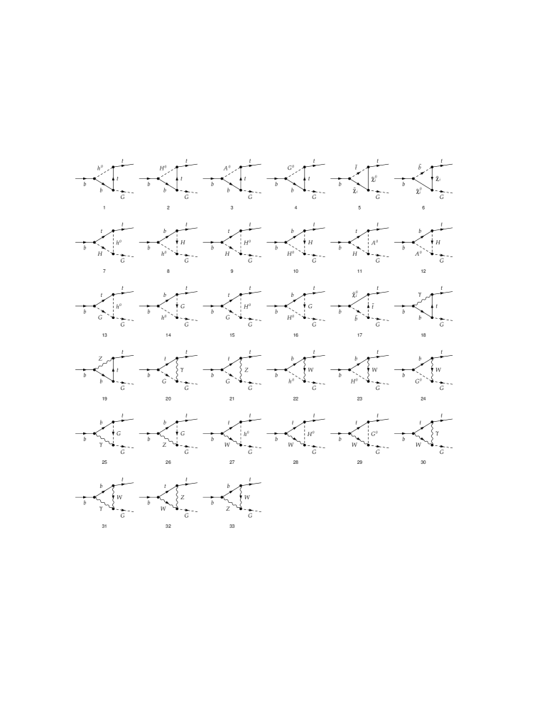
Figure 1: One loop triangle Feynman diagrams for the off-shell $b\to t\,G^{-}$.

First, in a diagrammatic analysis we observe that a linear ”gauge” logarithmic contribution ${1+2c^{2}_{W}\over 2s^{2}_{W}c^{2}_{W}}\,L(s)$ arises from $(VSq)$, $(SVq)$, $(qqVS)$ loops in the SM which then cancels with the additional $(\chi\chi\tilde{q})$ SUSY loop. The full list of triangle diagrams contributing the off-shell $b\to tG^{-}$ vertex is shown in Fig. (1). In the Yukawa sector a linear logarithmic term $-~{}{m^{2}_{a}\over 2s^{2}_{W}M^{2}_{W}}\,L(s)$ arises from the $(f^{\prime}fH_{SM})$, $(f^{\prime}fG^{0})$ triangles in the SM, whereas in the the MSSM the THDM structure ($\Phi_{1}$ coupled to down quarks, $\Phi_{2}$ coupled to up quarks) leads to the separate cancellation of $(f^{\prime}fH^{0})+(f^{\prime}fh^{0})$ and of $(f^{\prime}fG^{0})+(f^{\prime}fA^{0})$ contributions.

We then look in details at the splitting +PR analysis of $bg\to tG^{-}$ for the $b_{L}t_{R}$ amplitude (similar features appear for $b_{R}t_{L}$). The $b$ and $t$ splitting contributions are
in the SM ($L\equiv L(s)$)

$$c(t_{L})=c(b_{L})={1+26c^{2}_{W}\over 72s^{2}_{W}c^{2}_{W}}[3\,L-L^{2}]-{m^{2}_{t}+m^{2}_{b}\over 8M^{2}_{W}s^{2}_{W}}\,L$$ (5)

$$c(t_{R})={4\over 18c^{2}_{W}}[3\,L-L^{2}]-{m^{2}_{t}\over 4M^{2}_{W}s^{2}_{W}}\,L~{}~{}c(b_{R})={1\over 18c^{2}_{W}}[3\,L-L^{2}]-{m^{2}_{b}\over 4M^{2}_{W}s^{2}_{W}}\,L$$ (6)

and in the MSSM, with   $\tilde{m}^{2}_{t}=m^{2}_{t}(1+\cot^{2}\beta),~{}~{}\tilde{m}^{2}_{b}=m^{2}_{b}(1+\tan^{2}\beta)$   they are

$$c(t_{L})=c(b_{L})={1+26c^{2}_{W}\over 72s^{2}_{W}c^{2}_{W}}[2\,L-L^{2}]-2({\tilde{m}^{2}_{t}+\tilde{m}^{2}_{b}\over 8M^{2}_{W}s^{2}_{W}})\,L$$ (7)

$$c(t_{R})={4\over 18c^{2}_{W}}[2\,L-L^{2}]-({\tilde{m}^{2}_{t}\over 2M^{2}_{W}s^{2}_{W}})\,L~{}~{}c(b_{R})={1\over 18c^{2}_{W}}[2\,L-L^{2}]-({\tilde{m}^{2}_{b}\over 2M^{2}_{W}s^{2}_{W}})\,L$$ (8)

For $G^{-}$ splitting one has, in the SM

$$c(G^{-})={1+2c^{2}_{W}\over 8c^{2}_{W}s^{2}_{W}}[4\,L-\,L^{2}]-3{m^{2}_{t}+m^{2}_{b}\over 4s^{2}_{W}M^{2}_{W}}\,L$$ (9)

and in the MSSM (with $G^{-}H^{-}$ mixing contribution)

$$c(G^{-})={1+2c^{2}_{W}\over 8c^{2}_{W}s^{2}_{W}}[2\,L-\,L^{2}]-3{\tilde{m}^{2}_{t}\over 4s^{2}_{W}M^{2}_{W}}\,L$$ (10)

The PR contribution arising from the $b_{L}t_{R}G^{-}$ coupling is, in the SM

$$({\sqrt{2}m_{t}\over v})_{SM}={gm_{t}\over\sqrt{2}M_{W}}\to{\delta g\over g}+{\delta m_{t}\over m_{t}}-{\delta M_{W}\over M_{W}}$$

$$\to\{-~{}{51+30c^{2}_{W}\over 72s^{2}_{W}c^{2}_{W}}+3{3m^{2}_{t}+m^{2}_{b}\over 8s^{2}_{W}M^{2}_{W}}\}\,L$$ (11)

and in the MSSM

$$({\sqrt{2}m_{t}\over v_{2}})_{MSSM}\to{\delta g\over g}+{\delta m_{t}\over m_{t}}-{\delta M_{W}\over M_{W}}-{\delta\sin\beta\over\sin\beta}$$

$$\to\{-~{}{26+28c^{2}_{W}\over 36s^{2}_{W}c^{2}_{W}}+{6\tilde{m}^{2}_{t}+\tilde{m}^{2}_{b}\over 4s^{2}_{W}M^{2}_{W}}\}\,L$$ (12)

Concerning the gauge part one observes that the $G^{-}$ splitting contribution cancels with the PR part $\delta g/g-\delta M_{W}/M_{W}$ separately in the SM and in the MSSM, whereas the $b,t$ splitting and the PR part $\delta m_{q}/m_{q}$ combine to give ${1+2c^{2}_{W}\over 2s^{2}_{W}c^{2}_{W}}\,L$ in the SM but to cancel in the MSSM due to the addition of the $(\chi\tilde{q})$ bubble contributions to the quark self-energy. As an example, we show in Fig. (2) the full list of diagrams contributing the $b$ quark self-energy. For what concerns the Yukawa part, a similar property appears; $G^{-}$ splitting (including in MSSM the $G^{-}H^{-}$ mixing contribution) cancels with $-\delta M_{W}/M_{W}$ (and $\delta\tan\beta/\tan\beta$ in the MSSM) whereas the $b,t$ splitting and the PR $\delta m_{q}/m_{q}$ combine to give $-~{}{m^{2}_{a}\over 2s^{2}_{W}M^{2}_{W}}\,L$ in the SM but also cancellation in the MSSM because of the THDM structure of the $(Hq)$ bubble contributions. The above SM residual term arises only from the scalar part $\Sigma_{S}$ of the quark self-energy and in MSSM it is cancelled by the additional SUSY contribution to $\Sigma_{S}$ in a way very similar to what happens in the diagrammatic analysis.

We then look at other processes. First we replace $W_{long}$ by $Z_{long}\simeq G^{0}$ and look at $bg\to bG^{0}$. We observe exactly the same properties. We then extend the same analysis to other types of Higgses. In the SM case, $bg\to bH_{SM}$ gives the same resulting non zero residual terms as the pure SM $bg\to bG^{0}$. In the MSSM $bg\to tH^{-}$, $bg\to bH^{0}$, $bg\to bh^{0}$, $bg\to bA^{0}$ behave similarly to $bg\to tG^{-}$ with the complete cancellation of the linear logarithms. In each case the procedure of cancellation can be identified either through the diagrams $(\chi\chi S)+(ffS)$ or in splitting+PR method through $(\chi\tilde{q})$ and $(Hq)$ contributions to the $\Sigma_{S}$ quark self-energy using the specific Higgs-quark-quark couplings and Higgs mixing. In Fig. (3), we give the list of vertex diagrams for the case $b\to tH^{-}$.

Driven by these SUSY considerations we made one more extension by considering the production of SUSY partners, i.e. charginos and neutralinos replacing longitudinal gauge bosons or Higgs bosons, with illustration in the processes $bg\to\tilde{t}\chi^{-}$ (Fig. (4)) and $bg\to\tilde{b}\chi^{0}$. The diagrammatic and splittting+PR analyses of the processes show the same properties as for gauge and Higgs bosons, reflecting the supersymmetric invariance of this curiosity. The results are simple when separating the gaugino and the higgsino components. For the gaugino components i.e. factorizing out the Wino mixing element Rosiek $Z^{\pm}_{1i}$ for charginos, or the Wino, Bino elements $Z^{N}_{2i}$, $Z^{N}_{1i}$ for neutralinos, one obtains the same pure quadratic logarithms coefficient for splitting+PR as for $W^{\pm},Z,\gamma$ and linear +quadratic logarithms coefficients for the associated quark and squark lines. For the Higgsino components, i.e. factorizing the mixing element $Z^{\pm}_{21}$ for charginos or factorizing $Z^{N}_{3i,4i}$ for neutralinos, one observes the cancellation of the complete set of linear logarithms leaving an amplitude with pure quadratic logarithms.

II.1 Connection with basic SUSY properties

The above analyses have shown that this cancellation of the linear logarithms is not an accident but is a specific SUSY property of the $qqH$ and $\tilde{q}q\tilde{H}$ renormalized vertices which directly reflect in the $bg$ processes. For the gauge part the cancellation occurs due to the contribution of the spartners (gauginos, squarks) and for the Yukawa part due to the specific spectrum of the THDM. To relate this observed cancellation to some basic SUSY property, which is what one would naturally guess, is not simple. One plausible possibility would be to relate the cancellation of linear logarithms to the non renormalization theorem of chiral vertices nrth1 ; nrth2 ; nrth3 . However, this is not completely straightforward as is discussed for instance in Kraus:2001kn . Indeed, if perturbation theory is done in the Wess-Zumino gauge, then supersymmetry is non-linearly realized and allows individual field renormalizations for all matter fields  Wess:1974jb . As a consequence chiral Green functions are superficially convergent only up to gauge-dependent field redefinitions. In the specific case of our calculation, one checks that the Yukawa contributions to the linear logarithm are exactly opposite to the UV divergence $\Delta$ (i.e. the combination $\Delta-L$ in the concerned diagrams). These contributions are essentially gaugeless and the NR theorem applies in its simplest form. Thus the cancellation of the various $\Delta$ also leads to the cancellation of the overall coefficient multiplying $L$. This is not the case in SM, the $\Delta$ cancellation occuring only in the total sum (triangles and counter terms) with no special non-renormalization rule. For what concerns the gauge part the relation between cancellations and general SUSY properties is less obvious to us because of the above considerations and indeed the chiral vertex is not convergent. Still, although we cannot honestly claim to have completely proved it, we shall regard the cancellation of linear logaritms in the complete amplitude as a gauge-invariant property, whose origin might be a consequence of the non renormalization theorem. We believe that a deeper investigation of this origin, certainly beyond the limits of this paper, would be motivated.

III Genuine tests of Supersymmetry

This specific SUSY property of the $qqH$ and $\tilde{q}qH$ renormalized vertices could generate genuine tests of supersymmetry. In fact, a direct comparison of the energy dependence of the cross sections (logarithmic fits of the experimental results) for processes involving these vertices should confirm the absence of linear logarithmss. With this purpose we list in Appendix A the explicit expressions of the one loop high energy amplitudes for a few typical cases. They may be used for comparison with experiments.

In addition one should note that these expressions contain only quadratic logarithms which involve no free parameter. All parameters are included in the Born terms. This allows to write simple relations among amplitudes and cross sections of several processes. They would constitute specific SUSY tests valid not only not only at the Born level, but also, at high energies, at one loop. In Appendix B we list them separately for the charged sector ($bg\to tW^{-}$, $bg\to tH^{-}$, $bg\to\tilde{t}\chi^{-}_{i}$) and for the neutral sector ($bg\to b\gamma$, $bg\to bZ$, $bg\to bH^{0}$, $bg\to bh^{0}$, $bg\to bA^{0}$, $bg\to\tilde{b}\chi^{0}_{i}$). These relations generalize the simpler ones written for the pure gauge/gaugino cases $ug\to dW$ and $ug\to\tilde{d}\chi^{+}$ in ugdw .

Note that specific relations also appear among Higgs production processes. The importance of the processes $bg\to b+$ Higgs has been for example emphasized in ref.camp . As shown explicitely in Appendices A,B the amplitudes for Higgs production at Born level are related as

$${F^{H^{-}}_{-++}\over m_{t}\cot\beta}={F^{H^{-}}_{+--}\over m_{b}\tan\beta}=-~{}{2\cos\beta\over m_{b}\cos\alpha}~{}F^{H^{0}}_{\pm\mp\mp}={2\cos\beta\over m_{b}\sin\alpha}~{}F^{h^{0}}_{\pm\mp\mp}$$

$$=\mp{2i\over m_{b}\tan\beta}~{}F^{A^{0}}_{\pm\mp\mp}=\pm{2i\over m_{b}}~{}F^{G^{0}}_{\pm\mp\mp}$$ (13)

For the corresponding Born cross sections this would give:

$${1\over(m^{2}_{t}\cot^{2}\beta+m^{2}_{b}\tan^{2}\beta)}~{}\sigma^{Born}(H^{-})={2\cos^{2}\beta\over m^{2}_{b}\cos^{2}\alpha}~{}\sigma^{Born}(H^{0})={2\cos^{2}\beta\over m^{2}_{b}\sin^{2}\alpha}~{}\sigma^{Born}(h^{0})$$

$$={2\over m^{2}_{b}\tan^{2}\beta}~{}\sigma^{Born}(A^{0})={2\over m^{2}_{b}}~{}\sigma^{Born}(G^{0})$$ (14)

But at one loop logarithmic level $H^{-}$ production gets specific correction $C_{\mp\pm\pm}$ coefficients (see App.A), different for $-++$ and $+--$ amplitudes, so that the first equality is violated. However the 4 neutral productions get the same one loop high energy corrections (see coefficients $N_{\mp\pm\pm}$ in App. A) and therefore the same leading high energy amplitudes so that the following relations remain valid at this level:

$${\sigma(H^{0})\over\cos^{2}\alpha}={\sigma(h^{0})\over\sin^{2}\alpha}={\sigma(A^{0})\over\sin^{2}\beta}={\sigma(G^{0})\over\cos^{2}\beta}$$ (15)

The relation with $\sigma(H^{-})$ is more complicated due to the presence of the different coefficients $C_{\mp\pm\pm}$, but it is well defined as these $N_{\mp\pm\pm}$ and $C_{\mp\pm\pm}$ coefficients only involve the parameters $\alpha$ and $\beta$.
This whole set of relations among Higgs boson production cross sections could therefore provide the starting points of checks of the THDM structure. Of course, this proposal should take into account the specific experimental possibilities of LHC. In this respect, we feel that the following facts should be preliminary evidentiated:

1) The considered ratios of different Higgs rates have the remarkable property of being independent of the involved parton distribution functions. The measurement of these rates would represent a relatively clean test of the adopted supersymmetric scheme.

2) The asymptotic expressions that we derived are expected to become valid at large energies. This would be probably more realistic at a future high luminosity sLHC collider sLHC . At LHC they might become relevant in the final sector of the available cm energy, and be potentially visible in a suitable final mass dependence of a differential plot, rather than in the total rate that would be affected by the lowest energy points.

3) Given the stressed relevance of the considered Higgs production processes ratios, we feel that their complete one-loop electroweak (and strong) calculation would be oportune. In this case, the clean request on the complete e.w. component of reproducing the simple logarithmic expressions would provide a strong extra check of the validity of the theoretical calculation. Also, it would allow to separate the low energy sector, theoretically more complicated but provided by a certain numerical program, and join it with the predicted asymptotic expressions, in principle valid at the extreme machine energy sector. This complete calculation is in fact already being performed by our groupbgth .

IV Conclusions and perspectives

In conclusion we can say that the peculiar feature that we discovered is one more example of the subtlety of SUSY which adds to well-known and spectacular ones related to the non renormalization theorem. We have shown that it could lead to observable consequences. We have treated the simplest cases observable at LHC namely the various $bg\to qH$ or $bg\to\tilde{q}\tilde{H}$ processes which directly reflect the property of the $bqH$ or $b\tilde{q}\tilde{H}$ vertices. But other processes involving these vertices could be studied. Among them the simplest ones are for example $q\bar{q}\to VH$, $\tilde{V}\tilde{H}$, $VV$, $\chi\chi$. Experimental analyses of these processes at LHC or at a next proton-proton collider might constitute an alternative test of some of the assumed details of the involved Supersymmetric model.

Appendix A: High energy amplitudes at one loop

Process $bg\to tW^{-}_{tr}$. Using the same notations as in ref.bgtw the leading high energy helicity amplitudes are (with the linear log terms [ln] denoted by $L$ only coming from $b$, $t$ lines):

$$F^{W}_{-\pm-\pm} \to F^{Born}_{-\pm-\pm}[1+{\alpha\over 4\pi}~{}C_{tr}]$$ (16)

$$F^{Born}_{-+-+}\to~{}{eg_{s}\over\sqrt{2}s_{W}}({\lambda^{l}\over 2})2\cos{\theta\over 2}~{}~{}~{}~{}~{}~{}F^{Born}_{----}\to~{}{eg_{s}\over\sqrt{2}s_{W}}({\lambda^{l}\over 2})({2\over\cos{\theta\over 2}})$$ (17)

$$C_{tr} = {1+26c^{2}_{W}\over 18s^{2}_{W}c^{2}_{W}}~{}L-[{m^{2}_{t}\over 2s^{2}_{W}M^{2}_{W}}(1+\cot^{2}\beta)+{m^{2}_{b}\over 2s^{2}_{W}M^{2}_{W}}(1+\tan^{2}\beta)]L$$ (18)

$$-\{{1\over 2s^{2}_{W}}[ln^{2}{-u\over m^{2}_{W}}+ln^{2}{-u\over m^{2}_{Z}}]+{1-10c^{2}_{W}\over 36s^{2}_{W}c^{2}_{W}}~{}ln^{2}{-t\over m^{2}_{Z}}~{}\}$$

Process $bg\to tW^{-}_{long}$. The leading amplitudes are (with no [ln] at all).

$$F^{W}_{\mp,\pm,\pm,0}=F^{Born}_{\mp,\pm,\pm,0}[1+{\alpha\over 4\pi}C_{\mp,\pm,\pm}]$$ (19)

with

$$F^{Born}_{-,+,+,0}=eg_{s}({\lambda^{l}\over 2}){m_{t}\over s_{W}M_{W}}\cos{\theta\over 2}({1-\cos\theta\over 1+\cos\theta})~{}~{}F^{Born}_{+,-,-,0}=eg_{s}({\lambda^{l}\over 2}){m_{b}\over s_{W}M_{W}}\cos{\theta\over 2}({1-\cos\theta\over 1+\cos\theta})$$ (20)

$$C_{-,+,+}=-{1\over 3c^{2}_{W}}\log^{2}\frac{s}{m^{2}_{Z}}-{1\over 9c^{2}_{W}}\log^{2}\frac{-t}{m^{2}_{W}}+{1-4c^{2}_{W}\over 12s^{2}_{W}c^{2}_{W}}\log^{2}\frac{-u}{M_{Z}^{2}}-~{}{1\over 2s^{2}_{W}}\log^{2}\frac{-u}{M_{W}^{2}}~{}~{}$$ (21)

$$C_{+,-,-}=-{1+2c^{2}_{W}\over 12s^{2}_{W}c^{2}_{W}}\log^{2}\frac{s}{m^{2}_{Z}}-{1\over 2s^{2}_{W}}\log^{2}\frac{s}{m^{2}_{W}}+{1\over 18c^{2}_{W}}\log^{2}\frac{-t}{M_{W}^{2}}-~{}{1\over 6s^{2}_{W}}\log^{2}\frac{-u}{M_{W}^{2}}~{}~{}$$ (22)

Process $bg\to tH^{-}$. The amplitudes are expressed in terms of the same $C_{\mp,\pm,\pm}$ coefficients as in the previous $W_{long}$ case

$$F^{H^{-}}_{\mp,\pm,\pm} = F^{Born}_{\mp,\pm,\pm}\{1+[{\alpha\over 4\pi}]C_{\mp,\pm,\pm}\}$$ (23)

$$F^{Born}_{-,+,+}=-eg_{s}({\lambda^{l}\over 2}){m_{t}\over s_{W}M_{W}}\cos{\theta\over 2}({1-\cos\theta\over 1+\cos\theta})\cot\beta$$ (24)

$$F^{Born}_{+,-,-}=eg_{s}({\lambda^{l}\over 2}){m_{b}\over s_{W}M_{W}}\cos{\theta\over 2}({1-\cos\theta\over 1+\cos\theta})\tan\beta$$ (25)

Process $bg\to\tilde{t}_{a}\chi^{-}_{i}$. It is convenient to consider separately the gaugino and the higgsino components, using also the $\tilde{t}_{L}$ and $\tilde{t}_{R}$ decomposition. The gaugino component has only $[ln]$ from $b$, $\tilde{t}$ lines

$$F^{\chi}_{-++}(\tilde{t}_{L})=F^{Born}_{-++}(\tilde{t}_{L})\{1+{\alpha\over 4\pi}C_{tr}\}$$ (26)

with the same $C_{tr}$ as in the $W_{tr}$ case and

$$F^{Born}_{-++}(\tilde{t}_{L})=-g_{s}({\lambda^{l}\over 2})\sqrt{2}A^{L}_{i}(\tilde{t}_{L})\sin{\theta\over 2}~{}~{}~{}~{}~{}~{}~{}A^{L}_{i}(\tilde{t}_{L})=-~{}{e\over s_{W}}Z^{+}_{1i}$$ (27)

As in the $W_{long}$ case the higgsino components have no $[ln]$ at all :

$$F^{\chi}_{-++}(\tilde{t}_{R})=F^{Born}_{-++}(\tilde{t}_{R})[1+{\alpha\over 4\pi}C_{-++}]~{}~{}~{}~{}~{}F^{\chi}_{+--}(\tilde{t}_{L})=F^{Born}_{+--}(\tilde{t}_{L})[1+{\alpha\over 4\pi}C_{+--}]$$ (28)

$$F^{Born}_{-++}(\tilde{t}_{R})=-~{}{\alpha\over 4\pi}g_{s}({\lambda^{l}\over 2})\sqrt{2}A^{L}_{i}(\tilde{t}_{R})\sin{\theta\over 2}~{}~{}~{}~{}F^{Born}_{+--}(\tilde{t}_{L})=g_{s}({\lambda^{l}\over 2})\sqrt{2}A^{R}_{i}(\tilde{t}_{L})\sin{\theta\over 2}$$ (29)

$$A^{L}_{i}(\tilde{t}_{R})={em_{t}\over\sqrt{2}M_{W}s_{W}sin\beta}Z^{+}_{2i}~{}~{}~{}~{}~{}~{}~{}~{}A^{R}_{i}(\tilde{t}_{L})={em_{b}\over\sqrt{2}M_{W}s_{W}cos\beta}Z^{-*}_{2i}$$ (30)

Processes $bg\to b\gamma$ and $bg\to bZ_{tr}$. For future comparisons we separate the $B^{0}$ and $W^{0}$ components of $\gamma,Z$

$$F^{\gamma}_{\mp,\mu,\mp,\mu}=c_{W}F^{B0}_{\mp,\mu,\mp,\mu}+s_{W}F^{W0}_{\mp,\mu,\mp,\mu}~{}~{}~{}F^{Z}_{\mp,\mu,\mp,\mu}=c_{W}F^{W^{0}}_{\mp,\mu,\mp,\mu}-s_{W}F^{B0}_{\mp,\mu,\mp,\mu}$$ (31)

with

$$F^{B^{0}~{}Born}_{-+-+}=~{}{eg_{s}\over 6c_{W}}({\lambda^{l}\over 2})(2\cos{\theta\over 2})~{}~{}~{}~{}~{}F^{B^{0}~{}Born}_{----}=~{}{eg_{s}\over 6c_{W}}({\lambda^{l}\over 2})({2\over\cos{\theta\over 2}})$$ (32)

$$F^{B^{0}~{}Born}_{++++}=-~{}{eg_{s}\over 3c_{W}}({\lambda^{l}\over 2})(2\cos{\theta\over 2})~{}~{}~{}~{}~{}F^{B^{0}~{}Born}_{+-+-}=-~{}{eg_{s}\over 3c_{W}}({\lambda^{l}\over 2})({2\over\cos{\theta\over 2}})$$ (33)

$$F^{W^{0}~{}Born}_{-+-+}=~{}{eg_{s}\over 2s_{W}}({\lambda^{l}\over 2})(2\cos{\theta\over 2})~{}~{}~{}~{}~{}F^{W^{0}~{}Born}_{----}=~{}{eg_{s}\over 2s_{W}}({\lambda^{l}\over 2})({2\over\cos{\theta\over 2}})$$ (34)

and

$$F^{B^{0},W^{0}}_{-,\mu,-,\mu}=F^{B^{0},W^{0}~{}Born}_{-,\mu,-,\mu}[1+{\alpha\over 4\pi}C^{B^{0},W^{0},Born}_{tr,-}]$$ (35)

$$F^{B^{0}}_{+,\mu,+,\mu}=F^{B^{0}~{}Born}_{+,\mu,+,\mu}[1+{\alpha\over 4\pi}C^{B^{0},Born}_{tr,+}]$$ (36)

$$C^{B^{0},Born}_{tr,-}={1+26c^{2}_{W}\over 18s^{2}_{W}c^{2}_{W}}L-{\tilde{m}^{2}_{t}+\tilde{m}^{2}_{b}\over 2s^{2}_{W}M^{2}_{W}}L-[{1+8c^{2}_{W}\over 36s^{2}_{W}c^{2}_{W}}]ln^{2}t_{Z}-[{1\over s^{2}_{W}}]ln^{2}t_{W}$$ (37)

$$C^{B^{0},Born}_{tr,+}={1\over 9c^{2}_{W}}[2L-ln^{2}t_{Z}]-{\tilde{m}^{2}_{b}\over s^{2}_{W}M^{2}_{W}}[ln]$$ (38)

$$C^{W^{0},Born}_{tr,-}={1+26c^{2}_{W}\over 18s^{2}_{W}c^{2}_{W}}L-{\tilde{m}^{2}_{t}+\tilde{m}^{2}_{b}\over 2s^{2}_{W}M^{2}_{W}}L-{1+8c^{2}_{W}\over 36s^{2}_{W}c^{2}_{W}}ln^{2}t_{Z}+~{}{3-4s^{2}_{W}\over 2s^{2}_{W}(3-2s^{2}_{W})}ln^{2}t_{W}$$

$$-{3c^{2}_{W}\over 2s^{2}_{W}(3-2s^{2}_{W})}[ln^{2}s_{Z}+ln^{2}s_{W}+ln^{2}u_{Z}+ln^{2}u_{W}]$$ (39)

and one sees that $[ln]$ only arise from $b$ lines.

Process $bg\to bZ_{long}$. The leading amplitudes involves also only $ln^{2}$ terms:

$$F_{-++0}=F^{Born}_{-++0}\{1+{\alpha\over 4\pi}N_{-++}\}$$ (40)

$$F_{+--0} = F^{Born}_{+--0}\{1+{\alpha\over 4\pi}N_{+--}\}$$ (41)

$$F^{Born}_{-++0}\to-F^{Born}_{+--0}\to-~{}{eg_{s}\over 2s_{W}c_{W}}({\lambda^{l}\over 2}){\sqrt{2}m_{b}\over M_{Z}}\cos{\theta\over 2}({1-\cos\theta\over 1+\cos\theta})$$ (42)

$$N_{-++} = -~{}{1\over 6c^{2}_{W}}ln^{2}s_{Z}+~{}{1\over 18c^{2}_{W}}ln^{2}t_{Z}-~{}{1+2c^{2}_{W}\over 12c^{2}_{W}s^{2}_{W}}ln^{2}u_{Z}-~{}{1\over 2s^{2}_{W}}ln^{2}u_{W}$$ (43)

$$N_{+--} = -~{}{1+2c^{2}_{W}\over 12c^{2}_{W}s^{2}_{W}}ln^{2}s_{Z}-~{}{1\over 2s^{2}_{W}}ln^{2}s_{W}+~{}{1\over 18c^{2}_{W}}ln^{2}t_{Z}-~{}{1\over 6s^{2}_{W}}ln^{2}u_{Z}$$ (44)

Processes $bg\to bH^{0},bh^{0},bA^{0},bG^{0}$. The amplitudes are given in terms of the same $N_{\mp\pm\pm}$ as in the above $Z_{long}$ case (with no $[ln]$ at all)

$$F^{H}_{\mp,\pm,\pm} = F^{Born}_{\mp,\pm,\pm}[1+{\alpha\over 4\pi}N_{\mp\pm\pm}]$$ (45)

$$F^{Born}_{\mp,\pm,\pm}\to-~{}\sqrt{2}c^{L,R}g_{s}({\lambda^{l}\over 2})\cos{\theta\over 2}({1-\cos\theta\over 1+\cos\theta})$$ (46)

$$c^{L}_{H^{0}b}=c^{R}_{H^{0}b}=-~{}({em_{b}\over 2s_{W}M_{W}}){cos\alpha\over\cos\beta}~{}~{}~{}~{}~{}~{}~{}c^{L}_{h^{0}b}=c^{R}_{h^{0}b}=({em_{b}\over 2s_{W}M_{W}}){sin\alpha\over\cos\beta}$$ (47)

$$c^{L}_{A^{0}b}=c^{R*}_{A^{0}b}=(-i)({em_{b}\over 2s_{W}M_{W}})tan\beta~{}~{}~{}~{}~{}~{}c^{L}_{G^{0}b}=c^{R*}_{G^{0}b}=~{}(i)({em_{b}\over 2s_{W}M_{W}})$$ (48)

One can check the equivalence of $G^{0}$ with $Z_{long}$.

Process $bg\to\tilde{b}\chi^{0}_{i}$. Separating the gaugino (Wino, Bino) and the higgsino components and using the $\tilde{b}_{L}$, $\tilde{b}_{R}$ decomposition we obtain:

for the gaugino parts (with the same coefficients as in $\gamma,Z$ and only $[ln]$ from $b,\tilde{b}$ lines)

$$F_{+--}(\tilde{b}_{R})\to F^{Born~{}Bino}_{+--}(\tilde{b}_{R})\{1+{\alpha\over 4\pi}C^{B0}_{tr,+}\}$$ (49)

$$F_{-++}(\tilde{b}_{L})\to F^{Born~{}Bino}_{-++}(\tilde{b}_{L})\{1+{\alpha\over 4\pi}C^{B0}_{tr,-}\}+F^{Born~{}Wino}_{-++}(\tilde{b}_{L})\{1+{\alpha\over 4\pi}C^{W0}_{tr,-}\}$$ (50)

$$F^{Born~{}Bino}_{-++}(\tilde{b}_{L})={eg_{s}Z^{N}_{1i}\over 3c_{W}}({\lambda^{l}\over 2})\sin{\theta\over 2}~{}~{}~{}~{}~{}F^{Born~{}Wino}_{-++}(\tilde{b}_{L})=-~{}{eg_{s}Z^{N}_{2i}\over s_{W}}({\lambda^{l}\over 2})\sin{\theta\over 2}$$ (51)

For the higgsino parts (with the same coefficients as in the $Z_{long}$ case and no $[ln]$ at all)

$$F_{+--}(\tilde{b}_{L})\to F^{Born~{}Higg}_{+--}(\tilde{b}_{L})\{1+{\alpha\over 4\pi}N_{+--}\}$$

$$F_{-++}(\tilde{b}_{R})\to F^{Born~{}Higg}_{-++}(\tilde{b}_{R})\{1+{\alpha\over 4\pi}N_{-++}\}$$ (52)

$$F^{Born~{}Higg}_{+--}(\tilde{b}_{L})=F^{Born~{}Higg~{}*}_{-++}(\tilde{b}_{R})=-~{}{eg_{s}m_{b}\over M_{W}s_{W}\cos\beta}Z^{N*}_{3i}({\lambda^{l}\over 2})\sin{\theta\over 2}$$ (53)

Appendix B: SUSY relations

In the charged sector $W^{\pm},H^{\pm},\chi^{\pm}$, looking at the expressions of Appendix A for the high energy amplitudes and using in particular the fact that the one loop corrections for longitudinal gauge bosons and Higgses involve only squared logs without any free parameter, one obtains the relations

$$\cot{\theta\over 2}F^{\chi}_{-++}(\tilde{t}_{L})/Z^{+}_{1i}=-F^{W}_{-+-+}=-\cos^{2}{\theta\over 2}~{}F^{W}_{----}$$ (54)

$$F^{\chi}_{-++}(\tilde{t}_{R})/Z^{+}_{2i}=-\cot{\theta\over 2}~{}F^{W}_{-++0}/\sin\beta=\cot{\theta\over 2}~{}F^{H^{-}}_{-++}/\cos\beta$$ (55)

$$F^{\chi}_{+--}(\tilde{t}_{L})/Z^{-*}_{2i}=\cot{\theta\over 2}~{}F^{W}_{+--0}/\cos\beta=-\cot{\theta\over 2}~{}F^{H^{-}}_{+--}/\sin\beta$$ (56)

For polarized cross sections one gets

$$\sum_{i}{d\sigma(bg\to\chi^{-}_{i}+\tilde{t_{L}})_{-++}\over dcos\theta}=({ut\over u^{2}+s^{2}}){d\sigma(bg\to t+W^{-}_{T})\over dcos\theta}$$ (57)

$$\sum_{i}{d\sigma(bg\to\chi^{-}_{i}+\tilde{t_{R}})_{-++}\over dcos\theta}=({u\over t})[{d\sigma(bg\to t+W^{-}_{long})_{-++0}\over dcos\theta}+{d\sigma(bg\to t+H^{-})_{-++}\over dcos\theta}]$$ (58)

$$\sum_{i}{d\sigma(bg\to\chi^{-}_{i}+\tilde{t_{L}})_{+--}\over dcos\theta}=({u\over t})[{d\sigma(bg\to t+W^{-}_{long})_{+--0}\over dcos\theta}+{d\sigma(bg\to t+H^{-})_{+--}\over dcos\theta}]$$ (59)

and globally:

$$\sum_{i}[{d\sigma(bg\to\chi^{-}_{i}+\tilde{t_{L}})\over dcos\theta}+{d\sigma(bg\to\chi^{-}_{i}+\tilde{t_{R}})\over dcos\theta}]=({ut\over u^{2}+s^{2}})~{}{d\sigma(bg\to t+W^{-}_{T})\over dcos\theta}$$

$$+({u\over t})[{d\sigma(bg\to t+H^{-})\over dcos\theta}+{d\sigma(bg\to t+W^{-}_{long})\over dcos\theta}]$$ (60)

In the neutral sector $\gamma,Z,H^{0},h^{0},A^{0},\chi^{0}$

The relations among gaugino amplitudes are

$$F^{Wino}_{-++}(\tilde{b}_{L})/Z^{N}_{2i}=\tan{\theta\over 2}~{}F^{W}_{-+-+}=\tan{\theta\over 2}\cos^{2}{\theta\over 2}~{}F^{W}_{----}$$ (61)

$$F^{Bino}_{-++}(\tilde{b}_{L})/Z^{N}_{1i}=\tan{\theta\over 2}~{}F^{B}_{-+-+}=\tan{\theta\over 2}\cos^{2}{\theta\over 2}~{}F^{B}_{----}$$ (62)

$$F^{Bino}_{+--}(\tilde{b}_{R})/Z^{N*}_{1i}=\tan{\theta\over 2}~{}F^{B}_{+-+-}=\tan{\theta\over 2}\cos^{2}{\theta\over 2}~{}F^{B}_{++++}$$ (63)

$$F^{Wino}_{+--}(\tilde{b}_{R})=F^{W}_{+,\mu,+,\mu}=0$$ (64)

and among Higgsino amplitudes

$$F^{\chi}_{+--}(\tilde{b}_{L})=-{A^{0R}_{i}(\tilde{b}_{L})\over c^{R}_{H}}\cot{\theta\over 2}~{}F^{H}_{+--}$$ (65)

$$F^{\chi}_{-++}(\tilde{b}_{R})={A^{0L}_{i}(\tilde{b}_{R})\over c^{L}_{H}}\cot{\theta\over 2}~{}F^{H}_{-++}$$ (66)

They are valid for any $bH$ final state using the appropriate $H$ coupling $c^{L,R}$ given in Appendix A and

$$A^{0L}_{i}(\tilde{b}_{R})=-~{}{em_{b}\over\sqrt{2}s_{W}M_{W}\cos\beta}Z^{N}_{3i}~{}~{}~{}~{}~{}A^{0R}_{i}(\tilde{b}_{L})=-~{}{em_{b}\over\sqrt{2}s_{W}M_{W}\cos\beta}Z^{N*}_{3i}$$ (67)

First notice the relations among the Higgs production amplitudes at Born level

$${F^{H^{-}}_{-++}\over m_{t}\cot\beta}={F^{H^{-}}_{+--}\over m_{b}\tan\beta}=-~{}{2\cos\beta\over m_{b}\cos\alpha}~{}F^{H^{0}}_{\pm\mp\mp}={2\cos\beta\over m_{b}\sin\alpha}~{}F^{h^{0}}_{\pm\mp\mp}$$

$$=\mp{2i\over m_{b}\tan\beta}~{}F^{A^{0}}_{\pm\mp\mp}=\pm{2i\over m_{b}}~{}F^{G^{0}}_{\pm\mp\mp}$$ (68)

For the Born cross section this would give:

$${1\over(m^{2}_{t}\cot^{2}\beta+m^{2}_{b}\tan^{2}\beta)}~{}\sigma^{Born}(H^{-})={2\cos^{2}\beta\over m^{2}_{b}\cos^{2}\alpha}~{}\sigma^{Born}(H^{0})={2\cos^{2}\beta\over m^{2}_{b}\sin^{2}\alpha}~{}\sigma^{Born}(h^{0})$$

$$={2\over m^{2}_{b}\tan^{2}\beta}~{}\sigma^{Born}(A^{0})={2\over m^{2}_{b}}~{}\sigma^{Born}(G^{0})$$ (69)

But at one loop logarithmic level $H^{-}$ production gets specific correction coefficients, different for $-++$ and $+--$ amplitudes, such that the first equality is violated. However the 4 neutral productions get the same one loop high energy corrections (see above) and the same leading amplitudes such that the following relations remain valid at this level:

$${\sigma(H^{0})\over\cos^{2}\alpha}={\sigma(h^{0})\over\sin^{2}\alpha}={\sigma(A^{0})\over\sin^{2}\beta}={\sigma(G^{0})\over\cos^{2}\beta}$$ (70)

Secondly we can relate the neutralino production cross sections to those of $\gamma,Z$ and Higgs production. Eq() gives directly these relations for the pure Bino, Wino and Higgsino cases. The cross section $\sigma_{i}$ for physical neutralino ($i=1,4$) production are then given by

$$\sigma_{i}=\sigma(Bino)|Z^{N}_{1i}|^{2}+\sigma(Wino)|Z^{N}_{2i}|^{2}+\sigma(Higgsino)|Z^{N}_{3i}|^{2}$$ (71)

We refrain to write the obvious but lengthy expressions of the Bino, Wino and Higgsino cross sections in terms of these physical cross sections by solving the above equation. Note nevertheless that there is no $Z^{N}_{4i}$ contribution in the processes $bg\to\tilde{b}\chi^{0}$ because in the THDM structure this 4th component only appear in the top quark sector. This implies one constraint among the set of physical cross sections. We just write the global relation obtained by using the orthogonality $\Sigma_{i}|Z^{N}_{ji}|^{2}=1$

$$\sum_{i}[{d\sigma(bg\to\chi^{0}_{i}+\tilde{b_{L}})\over dcos\theta}+{d\sigma(bg\to\chi^{0}_{i}+\tilde{b_{R}})\over dcos\theta}]=({ut\over u^{2}+s^{2}})~{}[{d\sigma(bg\to b\gamma)\over dcos\theta}+~{}{d\sigma(bg\to b+Z_{T})\over dcos\theta}]$$

$$+({u\over t})[{d\sigma(bg\to b+H^{0})\over dcos\theta}+{d\sigma(bg\to b+h^{0})\over dcos\theta}+{d\sigma(bg\to b+A^{0})\over dcos\theta}+{d\sigma(bg\to t+Z_{long})\over dcos\theta}]$$ (72)

with

$$~{}~{}~{}~{}{d\sigma(bg\to b+H^{0})\over dcos\theta}+{d\sigma(bg\to b+h^{0})\over dcos\theta}={d\sigma(bg\to b+A^{0})\over dcos\theta}+{d\sigma(bg\to t+Z_{long})\over dcos\theta}~{}~{}~{}~{}~{}~{}~{}~{}~{}~{}~{}~{}$$ (73)

Figure 2: One loop self-energy of the $b$ quark.

Figure 3: One loop triangle Feynman diagrams for the off-shell $b\to t\,H^{-}$.

Figure 4: One loop triangle Feynman diagrams for the off-shell $b\to\widetilde{t}\,\chi^{-}$.