Quantum correlation in disordered spin systems:
entanglement and applications to magnetic sensing

Abstract

We propose a strategy to generate a many-body entangled state in a collection of randomly placed, dipolarly coupled electronic spins in the solid state. By using coherent control to restrict the evolution into a suitable collective subspace, this method enables the preparation of GHZ-like and spin-squeezed states even for randomly positioned spins, while in addition protecting the entangled states against decoherence. We consider the application of this squeezing method to improve the sensitivity of nanoscale magnetometer based on Nitrogen-Vacancy spin qubits in diamond.

I Introduction

Entangled states have attracted much interest as intriguing manifestation of non-classical phenomena in quantum systems. The creation of a many-body entangled state is a critical requirement in many quantum information tasks, such as quantum computation and communication, as well as in measurement devices. Here we outline a novel approach to obtain many-body entangled states in a solid-state system of dipolarly coupled electronic spins. In order to achieve the generation of entanglement in the presence of disordered couplings we take advantage of the fine experimental control reached by magnetic resonance to constrain the evolution to a suitable collective subspace Rey et al. (2008). Furthermore, this restriction to a collective subspace protects the entangled state from decoherence, thus bringing into experimental reach a particular class of entangled states (the spin squeezed states) that are of great practical interest. Spin squeezing in solid-state systems could have an immediate application to improve the sensitivity of recently demonstrated spin-based magnetometers Taylor et al. (2008); Maze et al. (2008); Balasubramanian et al. (2008). We show that controlling the naturally-occurring interactions to obtain a desired entangled state could yield a high sensitivity magnetometer in a nano-sized system for high-spatial resolution.

The paper is organized as follows. We first describe in section II entanglement generation in ideal and disordered systems, outlining the control techniques required to achieve the projection of the evolution to the desired subspace and its regimes of validity for different geometry distributions of the spins. In section III we then apply the method to spin squeezing and we show in section IV how the projection is also capable of reducing the noise effects, thus making squeezing advantageous for metrology. Finally in section V we present a possible implementation of the squeezing scheme. We focus our analysis on a system based on spin defects in diamond (Nitrogen-Vacancy center, NV L. Childress, et al. (2006); M.V.G. Dutt et al. (2007); Gaebel et al. (2006), Fig. 1 a). The NV electronic spins can be optically polarized and detected, and exhibit excellent coherence properties even at room temperature, allowing for a remarkable combination of sensitivity to external magnetic fields and high spatial resolution. We describe the operating regime of a spin squeezed NV magnetometer and the achievable sensitivity improvement. We emphasize that the described techniques are applicable to other spin systems, such as other paramagnetic impurities or trapped ions Rey et al. (2008).

II Entanglement generation

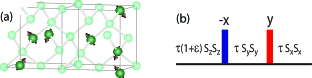
Figure 1: (a) System model: crystal with randomly placed electronic spins. (b) Control sequence: The Ising interaction is rotated along three axis to yield an isotropic interaction; adjusting the time delays, a small perturbation along the z direction is retained, to obtain the 1-axis squeezing operator.

II.1 Entanglement in ideal and disordered systems

We consider a solid-state system of N spin particles with two relevant internal states (0,1), each described by Pauli matrix operators $\sigma_{\alpha}^{k}$. Interactions among the spins can be used to generate entanglement. In particular, evolution of an initially uncorrelated state under the so-called one-axis squeezing Hamiltonian $\mathcal{H}^{1a}_{sqz}=dJ_{z}^{2}$ is known to create the multi-spin GHZ state (here we introduce the collective operator $J_{\alpha}=\sum_{k}S_{\alpha}^{k}$, with $S_{\alpha}^{k}=\frac{1}{2}\sigma_{\alpha}^{k}$). Starting from the fully polarized state along the $x$-direction $|{N/2,N/2}\rangle_{x}=\sum_{m_{z},\mu}C_{m_{z},\mu}|{N/2,m_{z},\mu}\rangle_{z}$, the different $m_{z}$-components acquire $m_{z}^{2}$ dependent phases that lead to collapse and revivals of the collective polarization $J_{x}$. At a time $t=\pi/(2d)$ the system is found in the collective GHZ state, $|{\psi_{GHZ}}\rangle_{x}=\frac{1}{\sqrt{2}}(|{N/2,N/2}\rangle_{x}+(-i)^{N+1}|{N/2,-N/2}\rangle_{x})$.

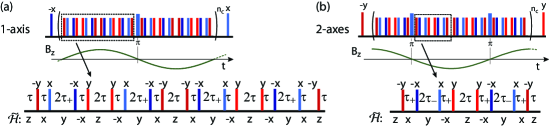
Figure 2: (Color online) Decoupling sequence. The narrow bars are $\pi/2$ pulses around different axis in the $m_{s}=\pm 1$ manifold, while the wide bars are $\pi$-pulses. The overall pulse sequence comprises 4 MREV8 sequences embedded in a spin echo sequence, with 34 pulses and a cycle time of $48\tau$. By varying the length of the time delays and the pulse phases, we obtain the squeezing Hamiltonians. The modified intervals are indicated by $\tau_{+}$ and $\tau_{-}$. For the one-axis squeezing (a) we obtain the first order Hamiltonian $\overline{\mathcal{H}}=(\mathcal{H}_{H}+\epsilon\mathcal{H}_{zz})/3$ (neglecting terms $\propto\epsilon\sin{\nu}^{2}$) and the linear Hamiltonian $S_{z}\rightarrow\sqrt{2}(S_{z}\cos{\nu}+S_{y}\sin{\nu})/3$. For the 2-axes case (b) the first order Hamiltonian is $\overline{\mathcal{H}}=(\mathcal{H}_{H}+\epsilon\mathcal{H}_{DQ})/3$ and the effective field is $(S_{y}-S_{x})/3$. $\tilde{\mathcal{H}}$ is the direction of the internal Hamiltonian in the interaction frame. $B_{z}$ is the AC field to be measured.

In most physical systems, however, the interactions among spins are not of the type described by the ideal entangling operator. Quite generally the Hamiltonian can be written as $\mathcal{H}_{zz}=\sum_{lj}d_{lj}S_{z,l}S_{z,j}$, where the couplings $d_{lj}$ are effectively limited to a finite number of neighbors. If it were possible to precisely engineer the strength of the couplings or the graph connectivity of the spins, it would still be possible to obtain a maximally entangled state such as the GHZ state Christandl et al. (2005); Franco et al. (2008). For example, even in the limit of nearest neighbor couplings only, a particular choice of couplings ($d_{k,k+1}=2d_{0}\sqrt{k(N-k)}/N$, with $d_{0}$ the maximum coupling strength) in the presence of a spatially-varying magnetic field $\mathcal{H}_{X}=\sum_{k}\sqrt{(2k-1)(2N-2k+1)}S^{k}_{x}$ creates the $N$-spin GHZ state in a time $d_{0}t=N\pi/8$.

In naturally occurring spin systems, where the couplings are usually given by the dipolar interaction scaling as $1/r^{3}$ with distance, it is difficult to engineer the couplings in the desired way and one has to deal with a disordered set of coupling strengths. We assume here an Ising interaction, $\mathcal{H}_{zz}$, with $d_{lj}=\frac{\mu_{0}g^{2}\mu_{D}^{2}}{4\pi\hbar}\frac{(3\hat{r}_{lj}.\hat{z}_{l}\hat{r}_{lj}.\hat{z}_{j}-1)}{r_{lj}^{3}}$. This is the case for an ensemble of NV electronic spins, where the zero-field splitting Hamiltonian $\Delta S_{z}^{2}$ is the largest quantizing energy scale (here we assume to operate in the $\pm 1$ manifold only, that constitutes an effective spin-$\frac{1}{2}$ system). This Hamiltonian will still generate entangled states, but the amount and type of entanglement may not be as desired.

II.2 Creating a global Hamiltonian

To obtain the desired high entangled state, we propose to create an effective collective Hamiltonian starting from a local one Rey et al. (2008). Notice that the projection of the $\mathcal{H}_{zz}$ Hamiltonian onto the $J=N/2$ subspace is given by:

$$P_{N/2}[\mathcal{H}_{zz}]=\frac{D}{(N-1)}(J_{z}^{2}-N\openone),$$ (1)

with $D=\frac{1}{N}\sum_{l,j}d_{lj}$. This operator can create the GHZ state, at the expenses of an increased evolution time. The restriction to the maximum angular momentum manifold can be achieved if $\mathcal{H}_{zz}$ is only a small perturbation to a stronger Hamiltonian that conserves the total angular momentum. In the following, we will show that with collective coherent control techniques it is possible to let the system evolve under the interaction:

$$\mathcal{H}_{H}^{1a}=\epsilon\mathcal{H}_{zz}+\mathcal{H}_{H}=\epsilon\sum_{lj}d_{lj}S_{z,l}S_{z,j}+\sum_{lj}d_{lj}\vec{S}_{l}\cdot\vec{S}_{j}$$ (2)

If $\epsilon\ll 1$, the Ising Hamiltonian is just a perturbation to the isotropic Heisenberg Hamiltonian $\mathcal{H}_{H}$, and to first order approximation, we only retain its projection on the $J=N/2$ manifold. Notice however that the squeezing Hamiltonian strength is now $\frac{\epsilon~{}D}{N-1}$, so that it is necessary to apply the squeezing interaction for a time increasing with the number of spins: $t\approx\frac{\pi}{2}\frac{N}{\epsilon D}$.

To obtain the desired Hamiltonian $\mathcal{H}_{H}^{1a}$, we propose to apply control techniques based on fast modulation of the internal Hamiltonian by cyclic sequences of pulses. These techniques have been used in NMR to obtain a wide range of desired interactions (see Appendix A). By cyclically rotating the Ising interaction among three perpendicular axis, it becomes on average isotropic (Fig. 1-b) . More complex modulation sequences (such as Mrev8 Rhim et al. (1973); Mansfield (1971)), achieve the averaging to higher order in $\left\|\mathcal{H}~{}t\right\|$. By a careful adjustment of the delays between pulses, it is possible to retain part of the $\mathcal{H}_{zz}$ Hamiltonian, so that the effective Hamiltonian is $\overline{\mathcal{H}}=\frac{1}{3}\mathcal{H}_{H}^{1a}$ (see Fig. 2.a).

The validity of the approximation taken in considering only the projection of $\mathcal{H}_{zz}$ onto the ground state $J=N/2$ manifold relies on the existence of an energy gap between the ground state manifold and the $J<N/2$ manifolds, induced by the isotropic interaction $\mathcal{H}_{H}$. The magnitude (and existence) of this gap depends on the geometry and spin-spin couplings of the system. For a 1D system with constant nearest-neighbor couplings $d_{0}$ the energy gap $E_{g}$ decreases as $d_{0}/N^{2}$, thus we must take $\epsilon\propto 1/N^{2}$ to always remain in the regime of validity of the approximation: the time required to achieve the GHZ state increases rapidly with the number of spins. The nearest-neighbor, 1D model is the worst case scenario; more generally, the time required will be a function of the dependence of $E_{g}$ and $D$ on $N$. For example, for a dipolarly coupled regular 1D system, $D=\zeta(3)d_{0}$ and the gap scales as $E_{g}\sim(d_{0}/N^{2})\log{N}$, with $d_{0}$ the coupling at the minimum distance $r_{0}$.

Better scaling can be achieved in a quasi-2D system, consisting of layers of spin impurities. Already a nearest-neighbor square lattice will have $E_{g}\sim d_{0}/N$ (it is in general $E_{g}\sim N^{-2/dim}$, where $dim$ is the system dimensionality), while for couplings decaying with distance as $r^{-3}$, $D\approx 7d_{0}$ and the gap is $E_{g}\sim d_{0}/\sqrt{N}$. In this case, the evolution time must increase with the spin number as $t\sim N^{3/2}$. A similar scaling is predicted if the spins have random spatial locations with density $n_{s}$. The gap can be estimated from the minimum coupling strength $E_{g}\sim d_{min}\frac{N}{2}$ with $d_{min}\sim(\frac{n_{s}}{N})^{3/dim}$ (where we assumed all the couplings to be positive). Thus we obtain again the same scaling of the gap energy $E_{g}\sim 1/\sqrt{N}$ in 2D and a constant gap in 3D. This last result, however, must be taken with caution, since the angular dependence of the dipolar couplings in 3D unavoidably gives rise to negative couplings; in that case not only the gap could even disappear, but the average coupling strength $D$ is zero for an isotropic spatial distribution. For finite size systems, however, because of the large variance of the couplings, a better estimate for $D$ is given not by the average but by the median of the dipolar coupling: $D\approx\textrm{median}\left[(3\cos{\vartheta}^{2}-1)d_{0}r_{0}^{3}/r^{3}\right]\approx\frac{2\pi}{3}d_{0}r_{0}^{3}\frac{n_{s}}{N+2}$, and we expect to obtain a non-zero gap with high probability. Still, the times required to obtain the GHZ state increase rapidly with the spin number in all the possible configurations presented. We thus turn our attention to a different class of entangled states, whose preparation time under ideal conditions decreases with the number of spins. A set of states that possess this property are the so-called spin squeezed states, which are of particular interest in metrology tasks.

III Spin squeezing

Spin squeezed states are many-body states showing pairwise entanglement Wang and Sanders (2003) and reduced uncertainty in the collective spin moment in one direction Kitagawa and Ueda (1993). This reduction in the measurement uncertainty, achieved without violating the minimum uncertainty principle by a redistribution of the quantum fluctuations between non-commuting variables, can be exploited to perform metrology beyond the Heisenberg limit. One-axis twisting ($\mathcal{H}^{1a}_{sqz}$) and two-axis twisting [$\tilde{\mathcal{H}}^{2a}_{sqz}=i~{}d(J_{+}^{2}-J_{-}^{2})/2$] Hamiltonians have been proposed to achieve this goal Kitagawa and Ueda (1993).

The degree of squeezing of a spin ensemble is evaluated by the squeezing parameter $\xi$. Several definitions have been proposed, depending on the context Müstecaplıoğlu et al. (2002). If the focus is simply to describe a non-uniform distribution of the quantum fluctuations, the appropriate quantity is $\xi_{h}=\Delta J_{i}/\sqrt{J_{j}/2}$, where $\Delta J_{\alpha}$ is the uncertainty in the $\alpha\in\{x,y,z\}$ direction of the collective angular momentum and $J_{\beta}$ its expectation value in a different direction. When spin squeezing is instead used in the context of quantum limited metrology Wineland et al. (1994), the squeezing parameter should measure the improvement in signal-to-noise ratio for the measured quantity $\varphi$,

$$\xi=\Delta\varphi_{sqz}/\Delta\varphi_{0}=\sqrt{N}\frac{\Delta J_{z}}{\|\frac{\partial\langle J_{z}\rangle}{\partial\varphi}\|}$$ (3)

This definition is associated to Ramsey-type experiments, in which an external magnetic field is measured via the detection of the accumulated phase $\varphi$ due to the Zeeman interaction and the phase uncertainty for a product state is $\sim 1/\sqrt{N}$.

In the limit of large spin numbers, using the one and two-axis squeezing operator, the optimal squeezing parameters are $\xi_{1a}=\frac{3^{1/3}}{\sqrt{2}N^{1/3}}$, at a time $t_{1a}=\frac{3^{1/6}}{d~{}N^{2/3}}$ Kitagawa and Ueda (1993), and $\xi_{2a}\sim\sqrt{\frac{1+2\sqrt{3}}{2N}}$ at $t_{2a}\approx\frac{1}{d~{}N}\log{\frac{2N}{\sqrt{3}}}$ André and Lukin (2002); Stockton et al. (2003), respectively. The one-axis squeezing operator reduces the variance of the collective magnetic moment along a direction at a variable angle $\nu\approx 0$ in the y-z plane, while for the two-axis operator the uncertainty reduction is in the x-direction.

An arbitrary Hamiltonian $\mathcal{H}_{zz}$ can generate a squeezed state Wang et al. (2001), although the squeezing would be less than in the ideal case and it becomes difficult to predict the optimal squeezing time and direction. For example, in the limit where the interaction is limited to first neighbors, the maximum squeezing achievable is fixed (independent of N) and bounded by $\xi_{nn}\approx 0.73$ Sørensen and Mølmer (2001). We can nonetheless apply the techniques presented in the previous section to project out the ideal squeezing Hamiltonian from the natural occurring disordered interaction.

The same control techniques described above can also generate two-axis squeezing. A different choice of time delays (Fig. 2.b) will produce the Hamiltonian: ${\mathcal{H}}_{H}^{2a}=(\epsilon\mathcal{H}_{dq}+\mathcal{H}_{H})/3$, where we introduced the so-called double quantum Hamiltonian $\mathcal{H}_{dq}=\sum_{lj}d_{lj}(S_{x,l}S_{x,j}-S_{y,l}S_{y,j})$. This operator creates squeezing by a two-axis twisting mechanism: for $\epsilon\ll 1$, we only retain the projection of $\mathcal{H}_{dq}$ on the $J=N/2$ manifold, $P[H_{dq}]=\frac{D}{(N-1)}[(J_{x}^{2}-J_{y}^{2})-N\openone]$, which is equivalent to $\mathcal{H}_{sqz}^{2a}=d(J_{x}^{2}-J_{y}^{2})/2$ (a 2-axis squeezing operator with optimum squeezing direction along the $\pi/4$ axis in the x-y plane). With this operator a squeezing parameter $\xi_{2a}\sim 2/\sqrt{N}$ can be achieved in a time $t_{2a}\approx\frac{(N-1)}{\epsilon D~{}N}\log{\left(\frac{2N}{\sqrt{3}}\right)}$: notice that the two-axis squeezing operator provides not only a better optimal squeezing, but also in a shorter time than the one-axis operator ($t_{1a}\approx\frac{3^{1/6}}{\epsilon D}N^{1/3}$). It is also possible to embed the control sequence within a spin-echo scheme, as needed for the control of dephasing due to a quasi-static spin bath Taylor et al. (2008), as well as to adjust the pulse phases in order to obtain an average external field operator acting on the direction of maximal squeezing.

IV Protection against the noise

Entangled states are known to decay more rapidly due to dephasing than separable states, so that in practice the improvement in sensitivity is often counterbalanced by the need to reduce the interrogation time Huelga et al. (1997); Auzinsh et al. (2004). In particular, if the system is prepared in the maximally entangled state (an N-particle GHZ state) the sensitivity improvement is completely lost in the presence of some classes of decoherence (single particle dephasing) Huelga et al. (1997), as the system is $N$-time more sensitive both to the signal and the noise. A partially entangled state, such as a spin squeezed state, can instead provide an advantage over separable states Ulam-Orgikh and Kitagawa (2001).

In the solid-state systems here considered the source of decoherence is usually the interaction of the electronic spins with other paramagnetic impurities and with nuclear spins. In the case of the NV electronic spins, the noise is caused by nitrogen electronic spins and by ¹³C nuclear spins. Since the couplings to these spins are much smaller than the zero-field splitting, they can only cause dephasing but not spin flips. The noise can be modeled as a fluctuating local magnetic field and represented by a single-spin dephasing stochastic Hamiltonian, $\mathcal{H}_{noise}=\sum_{k}\omega_{N}^{k}(t)S_{z}^{k}$; $\omega_{N}^{k}(t)$ are assumed to be independent stationary Gaussian random variables with zero mean and correlation function $\overline{\omega_{N}^{k}(t_{1})\omega_{N}^{h}(t_{2})}=\Omega_{k}f_{k}(t_{2}-t_{1})~{}\delta_{k,h}$. This noise leads to a decay of the average magnetization in the transverse direction: $\overline{\langle J_{x}(t)\rangle}=e^{-N\Gamma t}J_{x}^{id}(t)$ with respect to the ideal case $J_{x}^{id}(t)$. Here we defined $\Gamma=\frac{1}{2t}\int_{0}^{t}dt_{1}\int_{0}^{t}dt_{2}\overline{\omega_{N}(t_{1})\omega_{N}(t_{2})}$ and the average noise: $\omega_{N}(t)=1/N\sum_{k}\omega_{N}^{k}(t)$. This decay affects both product and 1-axis squeezed states in the same way (since the squeezing operator commute with the noise). The angular momentum uncertainty for the squeezed state is also affected, so that the squeezing parameter has now the value:

$$\xi^{2}_{1a}=\frac{1+\frac{N-1}{4}e^{-N\Gamma t}[(1-e^{-N\Gamma t})+1/R]P(R-1)}{\cos{(dt)}^{2N-2}}$$

where $R=P/\sqrt{P^{2}+Q^{2}}$ [with $P=1-\cos^{N-2}{(2dt)}$ and $Q=4\sin{(dt)}\cos^{N-2}{(dt)}$, see appendix B].

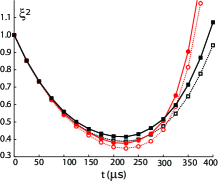
Figure 3: (Color online) Simulations (8 spins) of the squeezing parameter squared $\xi^{2}$ under 1-axis (squares) and 2-axis (circles) squeezing control schemes, with (solid lines) and without (dotted lines) the presence of noise. The noise was modeled by a random magnetic field in the z direction acting independently on each spin; noise parameters where $\Gamma=3$kHz, $\tau_{c}=100\mu s$. The spins were distributed randomly on the lattice of a quasi-2D diamond slab of depth 9nm and area $30\times 30$ nm. The density was $10^{18}\textrm{cm}^{-3}$ resulting in $D=.4$ MHz and $E_{gap}=50$kHz. The control sequence of Fig. 2 was used, with time delays of 1.4$\mu s$ and 1 to 12 cycles.

For small enough noise, such that the optimal squeezing time is shorter than the decoherence time, the squeezing parameter scales with the number of spins and decay rate as $\xi_{1a}\sim\frac{3^{1/3}}{N^{1/3}}\sqrt{\frac{1+(\Gamma/\epsilon D)^{2}}{2}}$. Only if the decoherence rate is such that $\Gamma/\epsilon D\sim 1$ we retain the ideal dependence of the squeezing parameter $\xi_{1a}\sim N^{-1/3}$. For stronger noise, the optimal time must be reduced and the maximum squeezing does not reach its optimal value.

The isotropic Hamiltonian $\mathcal{H}_{H}$ offers protection against the noise, provided this is smaller than the gap to the $J<N/2$ manifolds Rey et al. (2008). To first order approximation, the only part of the noise operator that has an effect on the system is its projection on the $J=N/2$ subspace: $\mathcal{H}_{noise}\rightarrow\omega_{N}(t)~{}J_{z}$. Not only the signal decays $N$-times slower, $\overline{\langle J_{x}(t)\rangle}=e^{-\Gamma t}J_{x}^{id}(t)$, but also the uncertainty is less affected. To provide a fairer comparison, we calculate a squeezing factor in which the non-squeezed state is also protected by the isotropic Hamiltonian:

$$\begin{array}[]{ll}\xi^{2}_{1a}=&\cos{(dt)}^{2-2N}\left\{1+\frac{N-1}{4}e^{-\Gamma t}\right.\\ &\left.\times[(1-e^{-\Gamma t})-2\sinh{(\Gamma t)}/P+1/R]P(R-1)\right\}\end{array}$$

The optimal squeezing now scales as $\xi_{1a}\sim\frac{3^{1/3}}{\sqrt{2}N^{1/3}}+\sqrt{\frac{\Gamma}{N~{}d}}$. We obtain a lower bound for the decoherence rate, $\Gamma/\epsilon D=o[N^{1/3}]$, that still allows optimal squeezing.

To take into account corrections to the truncation of the noise operator, we can follow the analysis in Rey et al. (2008) to find the leakage rate to the $N/2-1$ subspace. Because of the energy gap from the $J=N/2$ to the $J=N/2-1$ manifold (which can be populated by the flipping of one spin caused by the single-spin noise) the leakage outside the protected space is negligible, unless the energy gap to the first excitation is comparable with the cut-off energy $\omega_{c}$ of the noise (notice that $\omega_{c}=1/\tau_{c}$, the noise correlation time.)

While there is no analytical solution for the noise effects on the squeezing under the 2-axis Hamiltonian, we expect a similar advantage from the reduction of the noise to its collective part only. It is known that even the maximally entangled (GHZ) state does not exhibit a faster dephasing under collective noise Childs et al. (2000). Simulations for 8 spins show the expected improvement (Fig. [3]).

V Application to metrology: magnetic sensing and decoherence

We now describe an application of electronic spin squeezed states to precision magnetometry. Electronic spins in the solid state can be used to sense external magnetic fields, by monitoring the Zeeman phase shift between two sublevels via a Ramsey experiment. For small phase angle (weak fields) the signal measured (the total magnetization in the field direction) is proportional to the field.

The ideal sensitivity to the measured magnetic field for $M=T/t$ measurements and $N$ spins is given by

$$\Delta B_{z}=\frac{\hbar}{g\mu_{B}\sqrt{M}}\frac{\Delta J_{z}}{\|\frac{\partial\langle J_{z}\rangle}{\partial B_{z}}\|}=\frac{\hbar}{g\mu_{B}}\frac{1}{\sqrt{N~{}t~{}T}}\xi(t,N)$$ (4)

For sake of concreteness, we consider the recently proposed diamond-based magnetometer Taylor et al. (2008); Maze et al. (2008); Balasubramanian et al. (2008) (Fig. 4-a). The electronic spin associated to the NV in diamond is a sensitive probe of external, time-varying magnetic fields, due to its long coherence time and optical detection L. Childress, et al. (2006); M.V.G. Dutt et al. (2007). The electronic spin triplet can be polarized under application of green light and controlled by ESR pulses even at zero external magnetic field, thanks to the large zero-field splitting ($\Delta=2.87$GHz) (Fig. 4-b). In order to increase the interrogation time, a spin-echo based operating regime has been proposed, thus making the magnetometer sensitive to AC fields. The operating scheme of the magnetometer is depicted in Fig. 4. High spatial resolution is achieved by using for example a crystal of nanometer scales, which could be operated as a scanning tip. Sensitivity can be improved by increasing the number of NV’s in the tip, but this comes at the cost of errors introduced by the NV-NV couplings. Instead of refocusing these couplings Taylor et al. (2008), here we propose to use them to create a squeezed state.

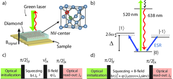
Figure 4: Magnetometer measurement scheme. a) A possible magnetometer setup, with NV center implanted in a slab of diamond. b) Optical and microwave control of a single NV center. Squeezing control sequences: c) A squeezed state is prepared before applying an external magnetic field to measure. d) Squeezing and Ramsey experiment are done simultaneously

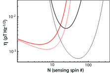
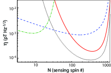
Figure 5: Sensitivity to an AC field with 22kHZ frequency, in a quasi 2D geometry [$V=(300\textrm{nm})^{2}\times 10\textrm{nm}$]. Left: Sensitivity for conversion efficiency $f=50\%$ (dotted lines) and $f=23\%$ (solid lines). Notice that only for $f\gtrsim 50\%$, the 2-axis squeezing approach (black lines) is preferable to the echo-only sequence (red lines). Right: Sensitivity for $f=.90$ (or equivalently, for a 30-fold increase in $T_{2}$ time thanks to refocusing, with respect to the $T_{2}$ at the highest conversion achieved Wee et al. (2007); Acosta et al. (2009)). Green line (dash-dotted): Sensitivity under spin-echo, without any refocusing of the spin-spin coupling. Blue dashed line: Sensitivity under Mrev8 sequence. The control sequence was repeated $n_{c}=6$ times with a delay between pulses of $\delta\tau=1.5\mu$s. Red line: Sensitivity under 1-axis squeezing, obtained with the same sequence parameters as above. Black dotted line: Sensitivity under 2-axis squeezing. The time delays $\tau_{+},\ \tau_{-}$ (see Fig. 2) were chosen in order to get an $\epsilon$ as small as needed to restrict the evolution to the protected manifold and the number of cycles increased as needed to obtain the optimal squeezing time.

Unfortunately, the coherence properties of high NV-density diamonds or nanocrystals Maze et al. (2008) are currently worse than for bulk, pure diamonds. NV’s are usually created by nitrogen implantation, followed by annealing that makes vacancies migrate and combine to the nitrogens Meijer et al. (2005); Rabeau et al. (2006). The current conversion efficiency $f$ is quite low (between 10% and 23% Wee et al. (2007)), thus interactions with the epr bath (in particular P1 nitrogen centers Hanson et al. (2008)) limit the coherence time and bound the allowed NV densities. The spin-echo signal is a function of the root-mean-square coupling among impurities and it decays exponentially as $e^{-t/T_{epr}}$. We find $T_{epr}\approx 4/[\frac{\mu_{0}}{4\pi}\frac{(g\mu_{B})^{2}}{\hbar}n_{epr}]$ Taylor et al. (2008), where the density of paramagnetic impurities is $n_{epr}=n_{s}(1-f)/f$ (with $n_{s}$ the NV center density). Not only the coherence time is short, but also the internal dynamics of the epr bath is fast, so that the protection provided by the gap created with the introduction of the isotropic Hamiltonian is not effective, as the condition $\omega_{c}\ll E_{gap}$ is no longer valid. Improved implantation schemes Greentree et al. (2006), coherent control techniques Taylor et al. (2008), polarization of the nitrogen, either at low temperature Takahashi et al. (2008) or by optical pumping, can reduce the effects of epr spins, up to the point where NV-NV couplings are the most important interactions. This is the regime suitable for squeezing. A conversion efficiency of 50% (or equivalently a 3 fold increase in the relaxation time due to the paramagnetic impurities) is needed to start seeing an advantage of the squeezing scheme over a simpler scheme based on repeated echoes (CPMG sequence Meiboom and Gill (1958)) as shown in Fig. 5(a).

VI Implementation in a diamond nano-crystal

If the material properties of NV-rich diamonds can be improved, a sizable squeezed state could be obtained in a nanocrystal (or in a suitably implanted portion of a bulk diamond, if surface effects are to be avoided). The residual decoherence mechanism is due to couplings to the nuclear spin bath (1% abundance of ¹³C), while spin relaxation occurs on timescales much longer than milliseconds and is thus neglected. The resultant decay of the signal, with a $T_{2}$ time on the order of $200-600\mu$s Takahashi et al. (2008); Maze et al. (2008), is about the same for a product state and for a squeezed state protected by the isotropic interaction. Errors in the creation of the average squeezing Hamiltonian $\bar{\mathcal{H}}$ by the multiple pulse sequence can be taken into account as a decaying term calculated from the third order average Hamiltonian Haeberlen (1976) and a moment expansion to second order Mehring (1983) (see Appendix A). For the Mrev8 sequence of Fig. 2, we obtain a decay term $\exp{\left(-{\tilde{\alpha}n_{s}^{6}t^{2}}\right)}$, where $t$ is the total averaging time and the coefficient $\tilde{\alpha}\sim(\frac{\mu_{0}}{4\pi}\frac{(g\mu_{B})^{2}}{\hbar})^{6}\tau^{4}$ depends on the actual NV-NV couplings ($\tau$ is the delay between pulses, see Fig. 2).

Taking into account the described effects, as well as the scaling of the field due to the control sequence and subunit efficiency $C$ of the optical read-out process, the sensitivity per root averaging time $\eta=\Delta B_{z}\sqrt{T}$ is:

$$\eta=\frac{\hbar}{g\mu_{B}}\frac{3\pi e^{[T/T_{2}]^{3}}e^{T/T_{epr}}}{C\sqrt{2nV~{}t}}e^{\tilde{\alpha}n_{s}^{6}T^{6}}\xi(t_{sqz},n_{s}V)$$ (5)

where $T=t+t_{sqz}$ is the total experimental time and $t$ is chosen to maximize the signal $t=t_{opt}$.

In order to reduce the total experiment time, to avoid decoherence, we would like to create squeezing while applying the external magnetic field. The total time would then be $T={max}(t_{sqz},t_{opt})$ instead of their sum and the interrogation time $t=T$ (See Fig. 4 c-d). For the 1-axis squeezing, if $\nu_{opt}$ were $0$, we could squeeze the spins while acquiring a phase from the external field since the two Hamiltonians would commute. More generally, since $Dt_{1a}$ and the accumulated phase $\varphi$ due to the external field are both small, we can approximate the desired evolution as

$$\begin{array}[]{l}e^{-i\varphi J_{z}}e^{-i\nu J_{x}}e^{-i\mathcal{H}_{sqz}^{1a}t_{1a}}\approx\\ e^{-i\nu J_{x}}\exp{\left[-i\varphi{(J_{z}\cos{\nu}+J_{y}\sin{\nu})}-i\mathcal{H}_{sqz}^{1a}t_{1a}\right]}.\end{array}$$

Provided one can rotate the external field in the $z$-$y$ plane by an angle $\nu$, the squeezing can be performed while the field is on. The error caused by this procedure is $\propto\varphi Dt_{1a}\sin{(\nu)}\sim\varphi D/N$ for large $N$. In the case of the two axis squeezing, as well, we can let the system rotate under the external field while squeezing provided the field is rotated in the $x$-$y$ direction; the error we introduce in this case is $\propto\varphi D\log{(N)}/N$.

In Fig. (5) we compare the sensitivity achievable with an uncorrelated state to the sensitivity provided by a 1-axis and 2-axis squeezed state. In particular, we can identify a region of parameters where the squeezing sequence offer an advantage over the simple echo control. We assumed to have implanted with a varying density of NV centers a quasi-2D region of a diamond of volume $V=(300\textrm{nm})^{2}$$\times$$10$nm (as this gives the best scaling with density). NV densities between $4$$\times$$10^{14}$cm^-3 and $8$$\times$$10^{16}$cm^-3 occupying a small 2D layer could be obtained via geometrically controlled ion implantation Schnitzler et al. (2009) of high purity diamond.

Notice that although the requirements for squeezing seem to be daunting, since the time to obtain an optimal squeezing could be long, the control needed is not more complex than what would be in any case required to simply refocusing the couplings. The many-body protected manifold succeeds into protecting the squeezed state in the environment envisioned (mainly composed by nuclear spins), since the noise correlation time is slow - on the order of millisecond as given by nuclear dipole-dipole interactions - while the couplings among NV centers can range up to hundreds of kHz because of the higher gyromagnetic ratio of electronic spins. In this situation, the gap offers a good protection against the noise; with the current implantation techniques, however, the nuclear bath effects are overwhelmed by the noise created by paramagnetic impurities, with much faster internal dynamics and we would expect the protection to fail there.

VII Conclusions

We described how spin squeezed states can be created in dipolarly coupled electronic spin systems and used for precision measurement of external magnetic fields. The key features of the method proposed are its applicability even to spin systems with random couplings and an intrinsic protection against single-spin noise. Although squeezed states are known to be more fragile to decoherence, in the present scheme the squeezing operator is in fact always accompanied by a many-body operator that provides protection to the squeezed state, reducing its dephasing rate to the rate of unsqueezed states. We studied the projected sensitivity gains for a particular application, an NV-based nanoscale magnetometer. As the control scheme needed to create an entangled state is not more demanding than the one required for the simple refocusing of the couplings, spin squeezing will provide a practical sensitivity enhancement in very high quality materials.

VIII Acknowledgments

We thank A.M. Rey and L. Jiang for stimulating discussions. This work was supported by ITAMP, the NSF, and the Packard Foundation.

IX Appendix

IX.1 Coherent averaging

Multiple pulse sequences (MPS) achieve the dynamical decoupling of unwanted interactions, or the creation of a desired one, using coherent averaging. By means of an external control the internal Hamiltonian is made time-dependent; using cyclic MPS and considering only stroboscopic measurements, the evolution is described by an effective Hamiltonian that, to leading order in time, is given by the time average of the modulated internal Hamiltonian. The evolution during a cycle can be better analyzed in the frame defined by the external control, where the internal Hamiltonian appears time-dependent and periodic: $\tilde{\mathcal{H}}_{int}(t)=U_{c}(t)^{\dagger}\mathcal{H}_{int}U_{c}(t)$. At times when $U_{c}(t)=\openone$, the evolution is given by $U(n_{c}t_{c})=(\mathcal{T}e^{-i\int_{0}^{t_{c}}\tilde{\mathcal{H}}_{int}(t)dt})^{n_{c}}$ (where $t_{c}$ is the cycle time and $n_{c}$ the number of cycles). The propagator can be rewritten using the Magnus expansion Magnus (1954):

$$U(t_{c})=\mathcal{T}e^{-i\int_{0}^{t_{c}}\tilde{\mathcal{H}}_{int}(t)dt}=e^{-i[\bar{H}^{(1)}+\bar{H}^{(2)}+\dots..]t_{c}},$$ (6)

where $\bar{H}^{(k)}$ are time-independent average Hamiltonians of order $k$ Haeberlen (1976). The MPS is tailored to produce the desired evolution usually up to the first or second order, and higher order terms lead to errors.

In the case of the Mrev8 sequence Mansfield (1971) shown in Fig. (2) time symmetrization brings to zero the second order terms Haeberlen (1976). The leading order error $\bar{\mathcal{H}}_{zz}^{(3)}$ cause dephasing of the spins. Its effects are captured by a moment expansion Mehring (1983) to second order of the effective Hamiltonian, $\langle T_{\varphi,6}^{2}\rangle=\textrm{Tr}\left[{[\bar{\mathcal{H}}^{(3)},J_{\perp}]^{2}}\right]/\textrm{Tr}\left[{J_{\bot}^{2}}\right]$, where $J_{\perp}=\sum_{k}S_{\perp,k}$ is the collective spin in a direction perpendicular to $z$. $\langle T_{\varphi,6}^{2}\rangle$ has actually the character of a sixth moment and its value is a function of the sixth power of the local field generated by the dipolar interaction. The sensitivity decay rate is thus proportional to the sixth order of the density and the square of the total time, with a coefficient $\tilde{\alpha}=\langle T_{\varphi,6}^{2}\rangle/n_{s}^{6}\sim(\frac{\mu_{0}}{4\pi}\frac{(g\mu_{B})^{2}}{\hbar})^{6}\tau^{4}$. Note that the Mrev8 sequence entails a large number of control pulses. For many typical errors (phase-lag and overshoot/undershoot) the refocusing is only affected at higher order. However, depolarizing pulse errors occurring with probability $p$ lead to a reduction of contrast: $C^{\prime}=C(1-p)^{k}$ for $k$ pulses. Using Mrev8 with echo gives $k=34$ and a requirement $p\lesssim 0.002$ for contrasts near unity.

IX.2 One axis-squeezing: analytical solution

Here we provide an analytical solution to the one-axis squeezing dynamics Kitagawa and Ueda (1993), which has been used to calculate the behavior in the presence of dephasing noise.

The one axis squeezing operator reduces the variance of the collective magnetic moment along a direction at a variable angle $\nu$ in the y-z plane. Defining $\chi=d~{}t$, we obtain :

$$\langle J_{x}\rangle=\frac{N}{2}\cos{\chi}^{N-1},\ \ \langle J_{y}\rangle=\langle J_{z}\rangle=0\\$$

$$\Delta J_{x}^{2}=\frac{N}{4}[N-\frac{N-1}{2}P]-\left(\frac{N}{2}\cos{\chi}^{N-1}\right)^{2}$$

$$\Delta J_{z}^{2}(\nu)=\frac{N}{4}\{1+\frac{N-1}{4}[P-\sqrt{P^{2}+Q^{2}}\cos{(2\nu+\textrm{atan}{\frac{Q}{P}})}]\}$$

where by $J_{z}(\nu)$ we indicate the operator $e^{i\nu J_{x}}J_{z}e^{-i\nu J_{x}}$ and we have set

$$\begin{array}[]{l}P=1-\cos^{N-2}{2\chi},\ \ \ Q=4\sin{\chi}\cos^{N-2}{\chi}\end{array}$$

The optimal value for $\nu$ (which minimize $\Delta J_{z}(\nu)$) is $\nu=-\frac{1}{2}\textrm{atan}{(Q/P)}$ [while $\nu=\pi/2-\frac{1}{2}\textrm{atan}{(Q/P)}$ would minimize $\Delta J_{y}(\nu)$]. Also notice that $\langle J_{y}(\nu)J_{x}\rangle=0$.

The squeezing parameter for this ideal case is:

$$\xi^{2}=\frac{[1+\frac{N-1}{4}(P-\sqrt{P^{2}+Q^{2}})]}{(\cos{\chi}^{N-1})^{2}}$$ (7)

For large spin systems and short times such that $N\chi^{2}\ll 1$ but $N\chi>1$, the optimal squeezing is obtained for $\chi_{1a}=\frac{3^{1/6}}{N^{2/3}}$, ($\nu\sim N^{-3}\approx 0$) and it scales with the number of spins as $\xi_{1a}=\frac{3^{1/3}}{\sqrt{2}N^{1/3}}$.

References

- Rey et al. (2008) A. M. Rey, L. Jiang, M. Fleischhauer, E. Demler, and M. D. Lukin, Phys. Rev. A 77, 052305 (2008).
- Taylor et al. (2008) J. M. Taylor, P. Cappellaro, L. Childress, L. Jiang, D. Budker, P. R. Hemmer, A. Yacoby, R. Walsworth, and M. D. Lukin, Nat. Phys. 4, 810 (2008), ISSN 1745-2473.
- Maze et al. (2008) J. R. Maze, P. L. Stanwix, J. S. Hodges, S. Hong, J. M. Taylor, P. Cappellaro, L. Jiang, A. Zibrov, A. Yacoby, R. Walsworth, et al., Nature 455, 644 (2008).
- Balasubramanian et al. (2008) G. Balasubramanian, I.-Y. Chan, R. Kolesov, M. Al-Hmoud, C. Shin, C. Kim, A. Wojcik, P. R. Hemmer, A. Krger, F. Jelezko, et al., Nature 445, 648 (2008).
- L. Childress, et al. (2006) L. Childress, et al., Science 314, 281 (2006).
- M.V.G. Dutt et al. (2007) M.V.G. Dutt et al., Science 316 (2007).
- Gaebel et al. (2006) T. Gaebel, M. Domhan, I. Popa, C. Wittmann, P. Neumann, F. Jelezko, J. R. Rabeau, N. Stavrias, A. D. Greentree, S. Prawer, et al., Nature Phys. 2, 408 (2006).
- Christandl et al. (2005) M. Christandl, N. Datta, T. C. Dorlas, A. Ekert, A. Kay, and A. J. Landahl, Phys. Rev. A 71, 032312 (2005).
- Franco et al. (2008) C. D. Franco, M. Paternostro, D. I. Tsomokos, and S. F. Huelga, Phys. Rev. A 77, 062337 (pages 10) (2008).
- Rhim et al. (1973) W.-K. Rhim, D. D. Elleman, and R. W. Vaughan, The Journal of Chemical Physics 58, 1772 (1973).
- Mansfield (1971) P. Mansfield, J. Phys. C 4, 1444 (1971).
- Wang and Sanders (2003) X. Wang and B. C. Sanders, Phys. Rev. A 68, 012101 (2003).
- Kitagawa and Ueda (1993) M. Kitagawa and M. Ueda, Phys. Rev. A 47, 5138 (1993).
- Müstecaplıoğlu et al. (2002) O. E. Müstecaplıoğlu, M. Zhang, and L. You, Phys. Rev. A 66, 033611 (2002).
- Wineland et al. (1994) D. J. Wineland, J. J. Bollinger, W. M. Itano, and D. J. Heinzen, Phys. Rev. A 50, 67 (1994).
- André and Lukin (2002) A. André and M. D. Lukin, Phys. Rev. A 65, 053819 (2002).
- Stockton et al. (2003) J. K. Stockton, J. M. Geremia, A. C. Doherty, and H. Mabuchi, Phys. Rev. A 67, 022112 (2003).
- Wang et al. (2001) X. Wang, A. Søndberg Sørensen, and K. Mølmer, Phys. Rev. A 64, 053815 (2001).
- Sørensen and Mølmer (2001) A. S. Sørensen and K. Mølmer, Phys. Rev. Lett. 86, 4431 (2001).
- Huelga et al. (1997) S. F. Huelga, C. Macchiavello, T. Pellizzari, A. K. Ekert, M. B. Plenio, and J. I. Cirac, Phys. Rev. Lett. 79, 3865 (1997).
- Auzinsh et al. (2004) M. Auzinsh, D. Budker, D. F. Kimball, S. M. Rochester, J. E. Stalnaker, A. O. Sushkov, and V. V. Yashchuk, Phys. Rev. Lett. 93, 173002 (2004).
- Ulam-Orgikh and Kitagawa (2001) D. Ulam-Orgikh and M. Kitagawa, Phys. Rev. A 64, 052106 (2001).
- Childs et al. (2000) A. M. Childs, J. Preskill, and J. Renes, Journal of Modern Optics 47, p155 (2000).
- Wee et al. (2007) T.-L. Wee, Y.-K. Tzeng, C.-C. Han, H.-C. Chang, W. Fann, J.-H. Hsu, K.-M. Chen, and Y.-C. Yu, J. Phys. Chem. A 111, 9379 (2007).
- Acosta et al. (2009) V. M. Acosta, E. Bauch, M. P. Ledbetter, C. Santori, K. C. Fu, P. E. Barclay, R. G. Beausoleil, H. Linget, J. F. Roch, F. Treussart, et al., ArXiv e-prints (2009), eprint 0903.3277.
- Meijer et al. (2005) J. Meijer, B. Burchard, M. Domhan, C. Wittmann, T. Gaebel, I. Popa, F. Jelezko, and J. Wrachtrup, Appl. Phys. Lett. 87, 261909 (2005).
- Rabeau et al. (2006) J. R. Rabeau, P. Reichart, G. Tamanyan, D. N. Jamieson, S. Prawer, F. Jelezko, T. Gaebel, I. Popa, M. Domhan, and J. Wrachtrup, Appl. Phys. Lett. 88, 023113 (2006).
- Hanson et al. (2008) R. Hanson, V. V. Dobrovitski, A. E. Feiguin, O. Gywat, and D. D. Awschalom, Science 320, 352 (2008).
- Greentree et al. (2006) A. D. Greentree, P. Olivero, M. Draganski, E. Trajkov, J. R. Rabeau, P. Reichart, B. C. Gibson, S. Rubanov, S. T. Huntington, D. N. Jamieson, et al., J. Phys.: Condens. Matter 18, S825 (2006).
- Takahashi et al. (2008) S. Takahashi, R. Hanson, J. van Tol, M. S. Sherwin, and D. D. Awschalom, Phys. Rev. Lett. 101, 047601 (2008).
- Meiboom and Gill (1958) S. Meiboom and D. Gill, Rev. Sc. Instr. 29, 688 (1958).
- Haeberlen (1976) U. Haeberlen, High Resolution NMR in Solids: Selective Averaging (Academic Press Inc., 1976).
- Mehring (1983) M. Mehring, Principle of High Resolution NMR in Solids (Springer-Verlag, 1983).
- Schnitzler et al. (2009) W. Schnitzler, N. M. Linke, R. Fickler, J. Meijer, F. Schmidt-Kaler, and K. Singer, Physical Review Letters 102, 070501 (pages 4) (2009).
- Magnus (1954) W. Magnus, Communications on Pure and Applied Mathematics 7, 649 (1954).