Ginzburg-Landau theory of a trapped Fermi gas with a BEC-BCS crossover

Abstract

The Ginzburg-Landau theory of a trapped Fermi gas with a BEC-BCS crossover is derived by the path-integral method. In addition to the standard Ginzburg-Landau equation, a second equation describing the total atom density is obtained. These two coupled equations are necessary to describe both homogeneous and inhomogeneous systems. The Ginzburg-Landau theory is valid near the transition temperature $T_{c}$ on both sides of the crossover. In the weakly-interacting BEC region, it is also accurate at zero temperature where the Ginzburg-Landau equation can be mapped onto the Gross-Pitaevskii (GP) equation. The applicability of GP equation at finite temperature is discussed. On the BEC side, the fluctuation of the order parameter is studied and the renormalization to the molecule coupling constant is obtained.

I Introduction

In a Fermi gas with a BEC-BCS crossover, the scattering length $a_{s}$ can be tuned by the technique of Feshbach resonance Feshbach . The effective interaction between atoms is proportional to the scattering length. A dilute Fermi gas with a negative scattering length is in a BCS pairing state below a critical temperature Jin ; Ketterle04 ; Thomas ; Chin2 , very similar to BCS superconductors. A dilute Fermi gas with a positive scattering length is in a BEC state of diatomic molecules below another critical temperature Jochim ; Greiner . Although the scattering length is divergent at the resonance, the system evolves smoothly between the BCS state and the molecular BEC state across the resonance at low temperatures. The observation of the BEC-BCS crossover Ketterle05 provided a new platform to study strong-correlation effects in fermionic systems.

The BEC-BCS crossover can be qualitatively understood in the BCS-type mean-field theoryleggett1980 ; eagles1969 . In this theory, as the interaction changes sign from attractive to repulsive across the resonance, the pair size of Cooper pairs decreases, and eventually these atom pairs become diatomic molecules. Although the mean-field theory offers the correct physical picture, it overestimates the critical temperature and the molecule-molecule scattering length in the weakly-interacting BEC limit. Nozières and Schmitt-Rink (NSR) NSR1985 found that fluctuation effects have to be considered to get the correct critical temperature. The total fermion density includes not only the mean-field fermion density but also the density of thermal molecules, which provides the important relation between the density and the chemical potential. The NSR theory is essentially equivalent to treating Gaussian fluctuations in the Ginzburg-Landau theory Randeria1993 . The NSR theory was also applied at zero temperature and the molecule-molecule scattering length was found in good agreement HuHui2006 ; Randeria2008 with the few-body calculation Petrov .

The purpose of this paper is to construct the Ginzburg-Landau theory to describe the BEC-BCS crossover in a trapped Fermi gas. Compared to microscopic theories, the Ginzburg-Landau theory has potential advantages of requiring less computation and being easier to be applied to inhomogeneous cases such as trapped systems. In the weakly-interacting BEC region, the Ginzburg-Landau equation was shown to be equivalent to the Gross-Pitaevskii (GP) equation at zero temperature GP-BdG . In the unitary region, a modified Ginzburg-Landau theory was developed to describe the phase slip yin1 , vortex yin2 , and vortex lattices yin3 . However there still lacks a complete Ginzburg-Landau description of the whole BEC-BCS crossover. In the following, we first derive the Ginzburg-Landau theory of a trapped Fermi gas by the functional-integral method, and obtain the Ginzburg-Landau equation and the equation for the fermion density. The density equation is important for providing the density profile of the BEC-BCS crossover in both the inhomogeneous and homogeneous cases. Then we concentrate on weakly-interacting BEC limit, study the Ginzburg-Landau equation at both zero and finite temperatures, and consider effects due to fluctuations of the order parameter. The conclusion is given in the end.

II Ginzburg-Landau theory of a trapped Fermi gas

A Fermi gas with a wide Feshbach resonance can be effectively described by a single-channel model, while for the narrow resonance case a two-channel model is more accurate Strinati . In this paper we consider only the wide resonance case in which the single-channel Hamiltonian density is given by

$${\mathscr{H}}(x)=\sum_{\sigma}\phi^{{\dagger}}_{\sigma}(x)\bigg{[}-\frac{\hbar^{2}\nabla^{2}}{2m}+V({\bf r})\bigg{]}\phi_{\sigma}(x)+g\phi^{{\dagger}}_{\uparrow}(x)\phi^{{\dagger}}_{\downarrow}(x)\phi_{\downarrow}(x)\phi_{\uparrow}(x),$$ (1)

where $x=({\bf r},\tau)$ is the coordinate in space and time, $\phi_{\sigma}(x)$ is the field operator of atoms with spin-component $\sigma$, $m$ is the mass of a Fermi atom, $V({\bf r})$ is the external trapping potential, and the coupling constant is given by $g=4\pi\hbar^{2}a_{s}/m$. In the following we consider only the spin-balanced case where the densities of spin-up and spin-down atoms are the same.

The grand partition function $Z$ can be written in functional-integral formalism as

$$Z=\int{\mathscr{D}}\phi^{*}_{\sigma}{\mathscr{D}}\phi_{\sigma}\exp[S_{\phi}],$$ (2)

with the action given by

$$S_{\phi}=\int{\mathrm{d}}^{4}x\bigg{\{}-\sum_{\sigma}\phi^{*}_{\sigma}(x)(\partial_{\tau}-\mu)\phi_{\sigma}(x)-{\mathscr{H}}[\phi^{*},\phi]\bigg{\}}$$ (3)

where $0\leq\tau\leq 1/(k_{B}T)$, and $\mu$ is the chemical potential.

The interaction term in Eq. (1) can be decoupled by introducing an auxiliary field $\Delta(x)$ and applying the Hubbard-Stratanovich transformation Randeria1993 . After integrating out the fermion field $\phi(x)$, we obtain

$$Z = \int{\mathscr{D}}\Delta^{*}{\mathscr{D}}\Delta\exp[S_{\Delta}],$$ (4)

where the action $S_{\Delta}$ is given in terms of the auxiliary field $\Delta$,

$$S_{\Delta}=\ln\det{\bf M}+{1\over g}\int{\mathrm{d}}^{4}x|\Delta(x)|^{2},$$ (5)

$${\bf M}=\bigg{[}\begin{array}[]{cc}-\partial_{\tau}-\hat{H}({\bf r})&-\Delta(x)\\ -\Delta^{*}(x)&-\partial_{\tau}+\hat{H}({\bf r})\end{array}\bigg{]},$$ (6)

and

$$\hat{H}({\bf r})=-\frac{\hbar^{2}\nabla^{2}}{2m}+V({\bf r})-\mu.$$ (7)

The action $S_{\Delta}$ can be further separated into two parts,

$$S_{\Delta}=S_{eff}+S_{0},$$ (8)

where $S_{0}=\ln\det{\bf M_{0}}$ is independent of $\Delta$ with

$${\bf M}_{0}=\bigg{[}\begin{array}[]{cc}-\partial_{\tau}-\hat{H}({\bf r})&0\\ 0&-\partial_{\tau}+\hat{H}({\bf r})\end{array}\bigg{]},$$ (9)

and the second part $S_{eff}$ vanishes when $\Delta=0$,

$$S_{eff} = \frac{1}{g}\int{\mathrm{d}}^{4}x|\Delta(x)|^{2}+{\rm Tr}\ln[{\bf I}-{\bf G}{\bf u}],$$ (10)

with ${\bf u}={\bf M}_{0}-{\bf M}=\bigg{[}\begin{array}[]{cc}0&\Delta(x)\\ \Delta^{*}(x)&0\end{array}\bigg{]}$, ${\bf I}$ as the identity matrix, and ${\bf G}={\bf M}^{-1}_{0}=\bigg{[}\begin{array}[]{cc}G_{+}&0\\ 0&G_{-}\end{array}\bigg{]}$ being the Green’s function of a noninteracting Fermi gas.

Next we expand the second term in $S_{eff}$ to the fourth order in $\Delta$. This approximation holds only when $\Delta$ is small compared to the Fermi energy, which is true when $|T-T_{c}|/T_{c}\ll 1$ or the system is in the weakly-interacting BEC regime. After the expansion, we obtain

$$S_{eff}\approx\frac{1}{g}\int{\mathrm{d}}^{4}x|\Delta(x)|^{2}+\int{\mathrm{d}}^{4}x{\mathrm{d}}^{4}x_{1}Q(x,x_{1})\Delta^{*}(x)\Delta(x_{1})$$

$$-\frac{1}{2}\int\prod_{i=1}^{4}{\mathrm{d}}^{4}x_{i}\,R(x_{1},...,x_{4})\Delta^{*}(x_{1})\Delta(x_{2})\Delta^{*}(x_{3})\Delta(x_{4}),$$

(11)

where

$$Q(x_{1},x_{2}) = -G_{+}(x_{1},x_{2})G_{-}(x_{2},x_{1}),$$

$$R(x_{1},...,x_{4}) = G_{+}(x_{1},x_{2})G_{-}(x_{2},x_{3})G_{+}(x_{3},x_{4})G_{-}(x_{4},x_{1}).$$

Since we are interested in low-energy and long-wavelength properties of the system, we apply gradient expansion in Eq. (11) and obtain

$$S_{eff} \approx \int{\mathrm{d}}^{4}x\bigg{[}\,d\,\Delta^{*}(x)\partial_{\tau}\Delta(x)+c\,\Delta^{*}(x)\frac{\hbar^{2}\nabla^{2}}{4m}\Delta(x)$$ (13)

$$+(a+\frac{1}{g})|\Delta(x)|^{2}-\frac{1}{2}b|\Delta(x)|^{4}\bigg{]},$$

where

$$a = \int{\mathrm{d}}^{4}x^{\prime}Q(x-x^{\prime}/2,x+x^{\prime}/2),$$

$$b = \int\prod_{i=1}^{3}{\mathrm{d}}^{4}x_{i}R(x,x_{1},x_{2},x_{3}),$$

$$c = \frac{4m}{\hbar^{2}}\int{\mathrm{d}}^{4}x^{\prime}\frac{{r^{\prime}}^{2}}{6}Q(x-x^{\prime}/2,x+x^{\prime}/2),$$ (14)

and $x^{\prime}=({\bf r}^{\prime},\tau^{\prime})$. The coefficient $d$ of the time-derivative term is defined as the coefficient of the linear term in the expansion of $Q$ in the frequency space in the zero-frequency limit,

$$d=\lim_{\omega\rightarrow 0}\int{\mathrm{d}}^{4}x^{\prime}{e^{i\omega\tau^{\prime}}-1\over i\omega}Q(x-x^{\prime}/2,x+x^{\prime}/2).$$ (15)

The equation of motion of the order parameter can be obtained by taking $\delta S_{eff}/\delta\Delta^{*}(x)=0$, which yields

$$(d\,\partial_{\tau}+c\,\frac{\hbar^{2}\nabla^{2}}{4m}+a+\frac{1}{g})\Delta(x)-b|\Delta(x)|^{2}\Delta(x)=0.$$ (16)

For an arbitrary trap potential $V({\bf r})$, it is difficult to obtain the exact analytical expression of the Green’s function ${\bf G}$. Here we consider only the case where the trap length is much larger than the inter-particle distance, and the local-density approximation (LDA) can be applied,

$${\bf G}(x_{1},x_{2})\approx{\bf G}^{(0)}(x_{1},x_{2}).$$ (17)

Here ${\bf G}^{(0)}=\bigg{[}\begin{array}[]{cc}G_{+}^{(0)}&0\\ 0&G_{-}^{(0)}\end{array}\bigg{]}$ is the Green’s function of a homogeneous noninteracting Fermi gas with the chemical potential $\mu^{\prime}=\mu-V[({\bf r}_{1}+{\bf r}_{2})/2]$,

$$\bigg{[}\begin{array}[]{cc}-\partial_{\tau}-\hat{T}+\mu^{\prime}&0\\ 0&-\partial_{\tau}+\hat{T}-\mu^{\prime}\end{array}\bigg{]}{\bf G}^{(0)}(x-x^{\prime})=\delta(x-x^{\prime}){\bf I},$$ (18)

where $\hat{T}=-\hbar^{2}\nabla^{2}/(2m)$. In LDA, the coefficients in Eq.(14) are given by

$$a = \int{{\mathrm{d}}^{3}k\over(2\pi)^{3}}\frac{\tanh[\epsilon_{\bf k}/(2k_{B}T)]}{2\epsilon_{\bf k}},$$

$$b = \int{{\mathrm{d}}^{3}k\over(2\pi)^{3}}\bigg{[}\frac{\tanh[\epsilon_{\bf k}/(2k_{B}T)]}{4\epsilon_{\bf k}^{3}}-\frac{\mathrm{sech}^{2}[\epsilon_{\bf k}/(2k_{B}T)]}{8k_{B}T\epsilon_{\bf k}^{2}}\bigg{]},$$

$$c = \int{{\mathrm{d}}^{3}k\over(2\pi)^{3}}\bigg{[}\frac{\tanh[\epsilon_{\bf k}/(2k_{B}T)]}{4\epsilon_{\bf k}^{2}}-\frac{\mathrm{sech}^{2}[\epsilon_{\bf k}/(2k_{B}T)]}{8k_{B}T\epsilon_{\bf k}}\bigg{]},$$

$$d = \int{{\mathrm{d}}^{3}k\over(2\pi)^{3}}\frac{\tanh[\epsilon_{\bf k}/(2k_{B}T)]}{4\epsilon^{2}_{\bf k}},$$ (19)

where $\epsilon_{\bf k}=\hbar^{2}k^{2}/(2m)-\mu^{\prime}$. It is important to note that in obtaining the coefficients given by Eq. (19) LDA is applied to the Green’s function of a noninteracting Fermi gas ${\bf G}^{(0)}$, which is different from applying LDA directly to the broken symmetry state. The latter case requires that the gap has to be much larger than the trap frequency, which does not hold near the critical temperature or in the weakly-interacting BEC regime.

In the unitary and BCS regime where there is a clear Fermi surface, the Fermion energy $\epsilon_{\bf k}$ has zero points, and there are divergences in integrands on r.h.s. of Eq. (19) at zero temperature, suggesting that this formalism does not work at zero temperature. At finite temperatures, the integrand on r.h.s. of the equation for the coefficient $d$ also diverges. A more careful treatment of this coefficient leads to damping in the dynamics of the order parameter Popov . In the following, we will not study the dynamics or zero-temperature properties in this regime so these issues do not occur.

At the stationary state, the function $\Delta({\bf r})$ satisfy the saddle-point condition

$${\delta S_{eff}\over\delta\Delta({\bf r})}=0,$$ (20)

which leads to the Ginzburg-Landau equation

$$-c\frac{\hbar^{2}}{4m}\nabla^{2}\Delta({\bf r})-(a+\frac{1}{g})\Delta({\bf r})+b|\Delta({\bf r})|^{2}\Delta({\bf r})=0.$$ (21)

The Ginzburg-Landau equation can be rewritten in terms of a wave-function $\psi({\bf r})$ defined by $\psi({\bf r})\equiv\sqrt{c}\Delta({\bf r})$,

$$-\frac{\hbar^{2}}{4m}\nabla^{2}\psi({\bf r})+\alpha\psi({\bf r})+\beta|\psi({\bf r})|^{2}\psi({\bf r})=0,$$ (22)

where

$$\alpha = -{1\over c}(a+{1\over g}),$$

$$\beta = {b\over c^{2}},$$ (23)

and the gradient terms of $c$ are ignored due to its small spatial variation within LDA. In Eq. (23), the coupling constant is given by

$$g^{-1}={m\over 4\pi\hbar^{2}a_{s}}-\int{{\mathrm{d}}^{3}k\over(2\pi)^{3}}{1\over 2\epsilon_{\bf k}^{0}},$$ (24)

where $\epsilon_{\bf k}^{0}=\hbar^{2}k^{2}/(2m)$, and the second r.h.s. term is a counter term in the particle-particle channel.

In the simple homogeneous case, the critical temperature $T_{c}$ is determined from the equation

$$\alpha=0,$$ (25)

which is exactly the $T_{c}$ equation in the mean-field BCS theory,

$$\int{{\mathrm{d}}^{3}k\over(2\pi)^{3}}\bigg{\{}\frac{\tanh[\epsilon_{\bf k}/(2k_{B}T_{c})]}{2\epsilon_{\bf k}}-\frac{1}{2\epsilon_{\bf k}^{0}}\bigg{\}}=-\frac{m}{4\pi\hbar^{2}a_{s}}.$$ (26)

Above $T_{c}$, the Ginzburg-Landau equation does not have a nontrivial solution. Close to $T_{c}$, to the first order of $T-T_{c}$, the coefficient $\alpha$ is approximately given by

$$\alpha\approx\lambda(T_{c})(T-T_{c}),$$ (27)

where

$$\lambda(T_{c})=\int{{\mathrm{d}}^{3}k\over(2\pi)^{3}}{1\over 4ck_{B}T_{c}^{2}}{\rm sech}^{2}[{\epsilon_{\bf k}\over 2k_{B}T_{c}}].$$

In the trapped case, the critical temperature $T_{c}$ is approximately determined by

$$\alpha({\bf r_{0}})=0,$$ (28)

where ${\bf r_{0}}$ is the place with the highest fermion density.

The Ginzburg-Landau equation determines the distribution of the order parameter in the stationary state. To obtain the density distribution, we need to study the thermodynamic potential $\Omega$, given by

$$\Omega=-k_{B}T\ln Z=\Omega_{f}+\Omega_{s},$$ (29)

where $\Omega_{f}$ is thermodynamic potential of a noninteracting Fermi gas, in LDA it is given by

$$\Omega_{f}=2\int{\mathrm{d}}^{3}r\int{{\mathrm{d}}^{3}k\over(2\pi)^{3}}[\epsilon_{\bf k}+k_{B}T\ln n_{\bf k}],$$ (30)

and $n_{\bf k}=1/\{1+\exp[\epsilon_{\bf k}/(k_{B}T)]\}$ is the Fermi distribution function. The term $\Omega_{s}$ is the contribution to thermodynamic potential by the order parameter. If we consider only the stationary state and ignore fluctuations of the order parameter in the mean-field approximation, $\Omega_{s}$ is approximately given by

$$\Omega_{s}^{(0)} = -k_{B}T\,S_{eff}^{(0)}$$

$$= \int{\rm d}^{3}r\left[-\psi^{*}({\bf r})\frac{\hbar^{2}}{4m}\nabla^{2}\psi({\bf r})+\alpha|\psi({\bf r})|^{2}+\frac{\beta}{2}|\psi({\bf r})|^{4}\right].$$

From the relation $N=-\partial\Omega/\partial\mu$, the atom density in the mean-field approximation can be obtained,

$$n({\bf r})\approx n_{f}({\bf r})+n_{s}^{(0)}({\bf r}),$$ (32)

where $n_{f}$ associated with $\Omega_{f}$ is the density of a homogeneous noninteracting Fermi gas with the chemical potential $\mu^{\prime}=\mu-V({\bf r})$ ,

$$n_{f}({\bf r})=2\int{{\mathrm{d}}^{3}k\over(2\pi)^{3}}n_{\bf k}({\bf r}),$$ (33)

and $n_{s}^{(0)}$ associated with $\Omega_{s}^{(0)}$ is the density due to the order parameter,

$$n_{s}^{(0)}({\bf r})\approx\frac{\partial a}{\partial\mu}|\Delta({\bf r})|^{2}=2|\psi({\bf r})|^{2}.$$ (34)

Note that in Eq. (34) the quartic term in $\psi({\bf r})$ is ignored because it is much smaller than the quadratic term. The density equation (32) indicates that the total density can be separated into two parts, i.e. $n_{f}$ from the normal state and $n_{s}^{(0)}$ from the superfluid order parameter, which is consistent with the two-fluid model of a superfluid at finite temperatures. The superfluid atom pairs are described by the wave-function $\psi({\bf r})$. In a trapped system, usually the total number of atoms $N$ is given,

$$N=\int{\mathrm{d}}^{3}rn({\bf r}),$$ (35)

from which the chemical potential $\mu$ can be solved. The Ginzburg-Landau equation (22) and the density equation (32) provide a complete mean-field phenomenological description of a trapped superfluid Fermi gas.

III Ginzburg-Landau equation in the weakly interacting BEC regime

In the weakly interacting BEC regime, the Fermi gas is dilute, $na_{s}^{3}\ll 1$, and the order parameter $\Delta$ is much less than the binding energy of a diatomic molecule given by $\epsilon_{0}=\hbar^{2}/(ma_{s}^{2})$. In this regime, since the chemical potential $\mu$ is negative, there is no Fermi surface. The coefficients in the Ginzburg-Landau equation given by Eq. (19) are well defined even at zero temperature. Therefore the Ginzburg-Landau theory can be applied from zero temperature to near $T_{c}$. In this section we study the Ginzburg-Landau equation in this regime.

At zero temperature, from Eq. (19) and (23), the coefficients in the Ginzburg-Landau equation are given by

$$\alpha_{0} = 4\sqrt{|\mu^{\prime}|}\big{(}\sqrt{|\mu^{\prime}|}-\sqrt{\epsilon_{0}/2}\big{)},$$

$$\beta_{0} = \frac{2\sqrt{2}\pi\hbar^{3}}{m^{3/2}\sqrt{|\mu^{\prime}|}},$$

$$d_{0} = c_{0}.$$ (36)

Since the density $n_{0}=|\alpha_{0}/\beta_{0}|$ is much smaller than $1/a_{s}^{3}$, we obtain $\mu^{\prime}=-(\epsilon_{0}/2)[1+{\rm O}(n_{0}a_{s}^{3})]$, and approximately

$$\alpha_{0} \approx -(2\mu^{\prime}+\epsilon_{0}),$$

$$\beta_{0} \approx \frac{8\pi\hbar^{2}a_{s}}{2m}.$$ (37)

With the time-dependent term, the Ginzburg-Landau equation can be written as

$$\partial_{\tau}\psi(x)-\frac{\hbar^{2}\nabla^{2}}{4m}\psi(x)+[2V({\bf r})-\mu_{b}]\psi(x)+\frac{8\pi\hbar^{2}a_{s}}{2m}|\psi(x)|^{2}\psi(x)=0,$$ (38)

where $\mu_{b}=2\mu+\epsilon_{0}$ is the chemical potential of molecules. This time-dependent Ginzburg-Landau equation is identical to the Gross-Pitaevskii equation of molecular BEC if the imaginary time $\tau$ is analytically continued to the real time $t$, $\tau=i\hbar t$, with $m_{b}=2m$ identified as the molecule mass and $a_{b}=2a_{s}$ identified as the scattering length between molecules. The density equation (32) in this regime is trivial, $n=2|\psi|^{2}$, which means all the atoms are paired into condensed molecules at zero temperature. However, the molecule scattering length $a_{b}$ extracted from Eq. (38) is $a_{b}=2a_{s}$, contradicting to the result $a_{b}\approx 0.6a_{s}$ from the few-body calculation Petrov . This discrepancy is due to the fact that we have not considered the fluctuation effect which are discussed in the next section.

In the weakly interacting regime, the BEC transition temperature $T_{c}$ is much smaller than the molecule binding energy $\epsilon_{0}$, $k_{B}T_{c}\ll\epsilon_{0}$. As a result, at any finite temperature below or near $T_{c}$, the coefficients in the time-dependent Ginzburg-Landau equation are almost the same as those at zero temperature given by Eq. (38), except the molecular chemical potential $\mu_{b}$ now varying with temperature. Therefore the time-dependent Ginzburg-Landau equation (38) remains valid at finite temperatures below or near $T_{c}$.

IV Fluctuation effects

In this section, we consider the effect due to the fluctuation of the order parameter which is ignored in our derivation so far. The effective action in terms of the pair wave-function $\psi(x)=\sqrt{c}\Delta(x)$ is given by

$$S_{eff} = \int{\rm d}^{4}x\bigg{[}\kappa\,\psi^{*}(x)\partial_{\tau}\psi(x)+\psi^{*}(x)\frac{\hbar^{2}}{4m}\nabla^{2}\psi(x)$$ (39)

$$-\alpha|\psi(x)|^{2}-\frac{1}{2}\beta|\psi(x)|^{4}\bigg{]},$$

where $\kappa=d/c$. For simplicity we consider only the homogeneous case. In the following, we concentrate on the weakly-interacting BEC regime near or below $T_{c}$, where $\kappa\approx 1$, $\alpha\approx-\mu_{b}$, and $\beta\approx 8\pi\hbar^{2}a_{s}/(2m)$. In this regime, the effective action given by Eq. (39) is the same action of a Bose gas with the boson mass given by $2m$ and a scattering length given by $2a_{s}$.

The effective action given by Eq. (39) provides a contribution to the thermodynamic potential given by

$$\Omega_{s}=-k_{B}T\ln\int\mathscr{D}\psi^{*}\mathscr{D}\psi\,\,\exp[S_{eff}],$$ (40)

from which we can obtain its contribution to the density $n_{s}$ by taking $-\partial\Omega_{s}/\partial\mu$. For a weakly-interacting Bose gas, Bogoliubov’s theory is accurate Fetter , in which $n_{s}$ is given by

$$n_{s}\approx 2\psi_{0}^{2}+\int{{\mathrm{d}}^{3}k\over(2\pi)^{3}}[{(\epsilon_{b{\bf k}}-\alpha)\over E_{b{\bf k}}}\coth({E_{b{\bf k}}\over 2k_{B}T})-1],$$ (41)

where $\epsilon_{b{\bf k}}=\hbar^{2}k^{2}/(4m)$ is the kinetic energy of a molecule, and $E_{b{\bf k}}=\sqrt{\epsilon_{b{\bf k}}(\epsilon_{b{\bf k}}-2\alpha)}$ is the excitation energy of the molecular quasi-particle. The order parameter $\psi_{0}$ is equivalent to the expectation value of the Bose field-operator, $\psi_{0}=\sqrt{-\alpha/\beta}$, where its phase is chosen so $\psi_{0}$ is positive for simplicity.

In Bogoliubov’s theory of a dilute Bose gas, there is an ultra-violet divergence appearing in the calculation of the thermodynamical potential $\Omega_{s}$ and the ground state energy, which is removed by the renormalization of the coupling constant

$$g_{b}^{-1}={2m\over 4\pi\hbar^{2}a_{b}}-\int{{\mathrm{d}}^{3}k\over(2\pi)^{3}}{1\over 2\epsilon_{b{\bf k}}},$$

where the second r.h.s. term is a counter term only appearing in the calculation involving the particle-particle channel. However in the effective action Eq. (39), the constant $\beta$ is not renormalized so far, which would result in a divergent term in $\Omega_{s}$ and the ground state energy Fetter2 given by

$$\Omega_{s}^{\prime}=-\alpha^{2}\sum_{\bf k}{1\over 4\epsilon_{b{\bf k}}}.$$ (42)

with the contribution to density given by

$$n_{s}^{\prime}=-\alpha\int{{\mathrm{d}}^{3}k\over(2\pi)^{3}}{1\over\epsilon_{b{\bf k}}},$$ (43)

where $\partial\alpha/\partial\mu\approx-2$. This ultra-violet divergence is an unphysical result, due to the invalidity of the gradient expansion used in derivation the Ginzburg-Landau action given by Eq. (13) at short distances. Fluctuations inside molecules become important at short distances, which is beyond the description of the gradient expansion. The energy scale at which the gradient expansion is invalid is approximately given by the molecule binding energy $\epsilon_{0}=\hbar^{2}/(ma_{s}^{2})$, which is equal to the molecular kinetic energy at wavevector $k=2/a_{s}$. Thus a straightforward renormalization method is to put a cutoff $\Lambda=2/a_{s}$ in the $k-$integrals of Eq. (42) and (43), which yields

$$n_{s}^{\prime}=-{4\alpha m\over\pi^{2}\hbar^{2}a_{s}}={16\over\pi}\psi_{0}^{2}.$$ (44)

After considering the renormalization due to fluctuations, we obtain the density equation,

$$n = n_{f}+n_{s}+n_{s}^{\prime}=2(1+{8\over\pi})\psi_{0}^{2}+\int{{\mathrm{d}}^{3}k\over(2\pi)^{3}}[{(\epsilon_{b{\bf k}}-\alpha)\over E_{b{\bf k}}}\coth({E_{b{\bf k}}\over 2k_{B}T})-\tanh({\epsilon_{\bf k}\over 2k_{B}T})].$$ (45)

At zero temperature, the density equation is simply given by

$$n = 2(1+{8\over\pi})\psi_{0}^{2}+\int{{\mathrm{d}}^{3}k\over(2\pi)^{3}}[{(\epsilon_{b{\bf k}}-\alpha)\over E_{b{\bf k}}}-1]$$ (46)

$$= 2(1+{8\over\pi})\psi_{0}^{2}+{16\over 3}\psi_{0}^{3}\sqrt{{8\over\pi}a_{s}^{3}}.$$

The first r.h.s term in Eq. (46) implies that the condensate density is $n_{0}=2(1+8/\pi)\psi_{0}^{2}$ not simply $2\psi_{0}^{2}$. The second r.h.s term is proportional to $\psi_{0}^{3}$, which comes from the quantum depletion of molecules. Thus in term of the true molecular condensate wave-function

$$\tilde{\psi}(x)=\sqrt{(1+8/\pi)}\psi(x),$$ (47)

the Ginzburg-Landau equation given by Eq.(38) should be rewritten as

$$\partial_{\tau}\tilde{\psi}(x)-\frac{\hbar^{2}\nabla^{2}}{4m}\tilde{\psi}(x)+[2V({\bf r})-\mu_{b}]\tilde{\psi}(x)+\frac{4\pi\hbar^{2}a_{b}}{2m}|\tilde{\psi}(x)|^{2}\tilde{\psi}(x)=0,$$ (48)

where $a_{b}$ is the scattering length of molecules after considering the renormalization,

$$a_{b}={2a_{s}\over 1+8/\pi}\approx 0.56a_{s},$$ (49)

very close to the result $a_{b}\approx 0.6a_{s}$ from the few-body calculation Petrov .

Figure 1: The molecule scattering length $a_{b}$ vs the cutoff $\Lambda$. The dotted lines are $\Lambda=2/a_{s}$, and $a_{b}=0.56a_{s}$ which is very close to the result $a_{b}\approx 0.6a_{s}$ from the few-body calculation Petrov . At $\Lambda=0$, the mean-field result $a_{b}=2a_{s}$ is recovered.

Although the renormalization to the mean-field molecule scattering length given by Eq. (49) was obtained below $T_{c}$, it is valid above $T_{c}$ as well, which can be understood in the vacuum renormalization of the molecule coupling constant in the $T$-matrix approximation,

$$g_{b}^{-1} = g_{b0}^{-1}-i\int{{\mathrm{d}}\omega\over 2\pi}\int{{\mathrm{d}}^{3}k\over(2\pi)^{3}}G_{b}({\bf k},\omega)G_{b}(-{\bf k},-\omega)$$ (50)

$$= g_{b0}^{-1}+\int{{\mathrm{d}}^{3}k\over(2\pi)^{3}}{1\over 2\epsilon_{b{\bf k}}},$$

where $g_{b0}=8\pi\hbar^{2}a_{s}/(2m)$ is the molecule coupling constant in the mean-field approximation, $g_{b}=4\pi\hbar^{2}a_{b}/(2m)$ is the renormalized coupling constant, and

$$G_{b}({\bf k},\omega)={1\over\omega-\epsilon_{b{\bf k}}+i\delta}$$

is the Green’s function of a molecule in vacuum. A cutoff $\Lambda=2/a_{s}$ should be put in the $k-$integral of Eq. (50) due to the same reason as stated above that this effective description cease to be accurate when $\epsilon_{b{\bf k}}\geq\epsilon_{0}$, leading to the same renormalization,

$$a_{b}={2a_{s}\over 1+4a_{s}\Lambda/\pi},$$ (51)

same as Eq. (49) at $\Lambda=2/a_{s}$. The molecule scattering length $a_{b}$ as a function of the cutoff $\Lambda$ is shown in Fig. 1. It should be emphasized that a more precise cutoff than $2/a_{s}$ is necessary for any further numerical comparison with the few-body result, which requires understanding of high-energy processes beyond the Ginzburg-Landau description. The vacuum renormalization of the molecule coupling constant can also be applied to trapped systems within LDA as long as the molecule binding energy is much bigger than trap frequencies.

At $T_{c}$, $\alpha=0$, the density is given by

$$n=2\int{{\mathrm{d}}^{3}k\over(2\pi)^{3}}\{{1\over\exp[\epsilon_{b{\bf k}}/(k_{B}T_{c})]-1}+{1\over\exp[\epsilon_{\bf k}/(k_{B}T_{c})]+1}\},$$ (52)

indicating that there are only thermally-excited atoms and molecules. Since $k_{B}T_{c}\ll\epsilon_{0}$, the number of thermally-excited atoms are negligiblly small, and almost all the particles are thermal molecules,

$$n\approx\int{{\mathrm{d}}^{3}k\over(2\pi)^{3}}{2\over\exp[\epsilon_{b{\bf k}}/(k_{B}T_{c})]-1}.$$ (53)

Generally at finite temperature below $T_{c}$, the density can be separated into the superfluid density $n_{sf}$ and the normal density $n_{n}$, $n=n_{sf}+n_{n}$. The superfluid density is given by the condensate density and the quantum depletion,

$$n_{sf}=2\tilde{\psi}_{0}^{2}\left(1+{8\over 3}\sqrt{\tilde{\psi}_{0}^{2}a_{b}^{3}\over\pi}\right),$$ (54)

consistent with traditional theories of a dilute Bose gas Fetter . The normal density is given by the total density of thermal atoms and molecules. Since the thermal atoms are negligible, the normal density is approximately given by the density of thermal molecules,

$$n_{n}=2\int{{\mathrm{d}}^{3}k\over(2\pi)^{3}}{(\epsilon_{b{\bf k}}-\alpha)\over E_{b{\bf k}}}{1\over\exp[E_{b{\bf k}}/(k_{B}T)]-1}.$$ (55)

Compared with the mean-field result in Eq (32), both the superfluid density and the normal density are renormalized. In the weakly-interacting BEC limit, as shown in Fig. 2, the renormalization to the density is quite strong. At zero temperature, the mean-field density account for only about 28% of the total density, while the rest density is due to fluctuation contribution. At $T_{c}$, almost all the density is due to fluctuation contribution.

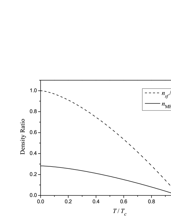
Figure 2: Density ratios of a homogeneous Fermi gas in the weakly-interacting BEC limit as functions of temperature. The solid line is the mean-field density given by Eq.(32) divided by the total density. For comparison, the dashed line is the ratio of the superfluid density to the total density.

Away from the weakly-interacting BEC limit, the fluctuation effect is more difficult to deal with in the Ginzburg-Landau theory. The coefficients in the Ginzburg-Landau equation are more complicated than those given by Eq. (36), and fluctuations of the order parameter cannot be simply treated by the Bogoliubov’s theory. Moreover the wavevector cutoff $2/a_{s}$ vanishes in the unitary region where a more subtle renormalization scheme is required. These problems will be explored in our future work. The situation is simpler again on the other side, in the weakly-interacting BCS limit, where the fluctuation of the order parameter is strongly damped. In this limit, the mean-field theory is accurate and the fluctuation of the order parameter is less important.

V Conclusion

In conclusion, we have derived the Ginzburg-Landau theory of a trapped Fermi gas with a BEC-BCS crossover. Two equations including the standard Ginzburg-Landau equation and the density equation are obtained to describe the order parameter distribution and the density profile. In the weakly-interacting BEC limit, the Ginzburg-Landau equation is equivalent to the Gross-Pitaevskii (GP) equation. The fluctuation of the order parameter is strong in this limit, which can be treated by the Bogoliubov’s theory. Compared with mean-field results, both the density and the molecule-molecule scattering length are renormalized, in agreement with the few-body and NSR theories. This work is supported by NSFC under Grant No. 10674007, and by Chinese MOST under grant number 2006CB921402.

References

• (1) H. Feshbach, Theoretical Nuclear Physics, (Wiley, New York, 1992).
• (2) C. A. Regal, M. Greiner, and D. S. Jin, Phys. Rev. Lett. 92, 040403 (2004).
• (3) M. W. Zwierlein, C. A. Stan, C. H. Schunck, S. M. F. Raupach, A. J. Kerman, and W. Ketterle, Phys. Rev. Lett. 92, 120403 (2004).
• (4) J. Kinast, S. L. Hemmer, M. E. Gehm, A. Turlapov, and J. E. Thomas, Phys. Rev. Lett. 92, 150402 (2004).
• (5) C. Chin et al., Science 305, 1128 (2004).
• (6) S. Jochim et al., Science 302, 2101 (2003).
• (7) M. Greiner, C. A. Regal, and D. S. Jin, Nature 426, 537 (2003).
• (8) M. W. Zwierlein, J. R. Abo-Shaeer, A. Schirotzek, C. H. Schunck, and W. Ketterle, Nature 435, 1047 (2005).
• (9) A. J. Leggett, in Modern Trends in the Theory of Condensed Matter, edited by A. Pekalski and R. Przystawa (Springer-Verlag, Berlin, 1980).
• (10) D. M. Eagles, Phys. Rev. 186, 456 (1969).
• (11) P. Nozières and S. Schmitt-Rink, J. Low Temp. Phys. 59, 195 (1985).
• (12) C. A. R. Sá de Melo, M. Randeria, and J. R. Engelbrecht, Phys. Rev. Lett. 71, 3202 (1993).
• (13) H. Hu, X.-J. Liu and P. D. Drummond, Europhys. Lett. 74, 574 (2006).
• (14) R. B. Diener, R. Sensarma, and M. Randeria, Phys. Rev. A 77, 023626 (2008).
• (15) D. S. Petrov, C. Salomon, and G. V. Shlyapnikov, Phys. Rev. Lett. 93, 090404 (2004).
• (16) P. Pieri and G. C. Strinati, Phys. Rev. Lett. 91, 030401 (2003).
• (17) L. Yin and P. Ao, Phys. Rev. A 71, 041603(R) (2005); H.-Y. Wu and L. Yin, Acta Physica Sinica 55, 490 (2006).
• (18) M. Gao, H.-Y. Wu, and L. Yin, Phys. Rev. A 74, 023604 (2006).
• (19) M. Gao and L. Yin, Int. J. Mod. Phys. B 22, 3967 (2008).
• (20) S. Simonucci, P. Pieri, and G. C. Strinati, Europhys. Lett. 69, 713 (2005).
• (21) V. N. Popov, Functional integrals and collective excitations, (Cambridge University, Cambridge, 1987), Chapter 13.
• (22) A. L. Fetter and J. D. Walecka, Quantum theory of many-particle systems, (McGraw-Hill, San Francisco, 1971), Chapter 10.
• (23) The divergence is in the first r.h.s term of Eq. (35.25) in Ref. Fetter .