RNA polymerase motors: dwell time distribution, velocity and dynamical phases

Abstract

Polymerization of RNA from a template DNA is carried out by a molecular machine called RNA polymerase (RNAP). It also uses the template as a track on which it moves as a motor utilizing chemical energy input. The time it spends at each successive monomer of DNA is random; we derive the exact distribution of these “dwell times” in our model. The inverse of the mean dwell time satisfies a Michaelis-Menten-like equation and is also consistent with a general formula derived earlier by Fisher and Kolomeisky for molecular motors with unbranched mechano-chemical cycles. Often many RNAP motors move simultaneously on the same track. Incorporating the steric interactions among the RNAPs in our model, we also plot the three-dimensional phase diagram of our model for RNAP traffic using an extremum current hypothesis.

I Introduction

RNA polymerase (RNAP) is a molecular motor schliwa . It moves on a stretch of DNA, utilizing chemical energy input, while polymerizing a messenger RNA (mRNA) gelles98 . The sequence of monomeric subunits of the mRNA is dictated by the corresponding sequence on the template DNA. This process of template-dictated polymerization of RNA is usually referred to as transcription alberts . It comprises three stages, namely, initiation, elongation of the mRNA and termination.

We first report analytical results on the characteristic properties of single RNAP motors. In our approach ttdc , each RNAP is represented by a hard rod while the DNA track is modelled as a one-dimensional lattice whose sites represent a nucleotide, the monomeric subunits of the DNA. The mechano-chemistry of individual RNAP motors is captured in this model by assigning $m$ distinct “chemical” states to each RNAP and postulating the nature of the transitions between these states. The dwell time of an RNAP at successive monomers of the DNA template is a random variable; its distribution characterizes the stochastic nature of the movement of RNAP motors. We derive the exact analytical expression for the dwell-time distribution of the RNAPs in this model.

We also report results on the collective movements of the RNAPs. Often many RNAPs move simultaneously on the same DNA track; because of superficial similarities with vehicular traffic css , we refer to such collective movements of RNAPs as RNAP traffic Klum03 ; polrev ; liverpool ; ttdc ; klumpp08 . Our model of RNAP traffic can be regarded as an extension of the totally asymmetric simple exclusion process (TASEP) schuetz for hard rods where each rod can exist at a location in one of its $m$ possible chemical states. The movement of an RNAP on its DNA track is coupled to the elongation of the mRNA chain that it synthesizes. Naturally, the rate of its forward movement depends on the availability of the monomeric subunits of the mRNA and the associated “chemical” transitions on the dominant pathway in its mechano-chemical cycle. Because of the incorporation of the mechano-chemical cycles of individual RNAP motors, the number of rate constants in this model is higher than that in a TASEP for hard rods. Consequently, we plot the phase diagrams of our model not in a two-dimensionl plane (as is customary for the TASEP), but in a 3-dimensional space where the additional dimension corresponds to the concentration of the monomeric subunits of the mRNA.

II Model

We take the DNA template as a one dimensional lattice of length $L$ and each RNAP is taken as a hard rod of length $\ell$ in units of the length of a nucleotide. Although an RNAP covers $\ell$ nucleotides, its position is denoted by the leftmost nucleotide covered by it. Transcription initiation and termination steps are taken into account by the rate constants $\omega_{\alpha}$ and $\omega_{\beta}$, respectively. A hard rod, representing an mRNA, attaches to the first site $i=1$ on the lattice with rate $\omega_{\alpha}$ if the first ${\ell}$ sites are not covered by any other RNAP at that instant of time. Similarly, an mRNA bound to the rightmost site $i=L$ is released from the system, with rate $\omega_{\beta}$. We have assumed hard core steric interaction among the RNAPs; therefore, no site can be simultaneously covered by more than one RNAP. At every lattice site $i$, an RNAP can exist in one of two possible chemical states: in one of these it is bound with a pyrophosphate (which is one of the byproducts of RNA elongation reaction and is denoted by the symbol $PP_{i}$), whereas no $PP_{i}$ is bound to it in the other chemical state (see fig.1). For plotting our results, we have used throughout this paper $\omega_{12}~{}=~{}31.4~{}s^{-1}$,$\omega_{12}^{b}~{}=~{}30.0~{}s^{-1}$ and $\omega_{21}^{f}~{}=~{}[NTP]~{}\tilde{\omega}_{21}^{f}~{}s^{-1}$, where $[NTP]$ is concentration of nucleotide triphosphate monomers (fuel for transcription elongation) and $\tilde{\omega}_{21}^{f}~{}=~{}10^{6}~{}M^{-1}s^{-1}$.

Figure 1: The mechano-chemical cycle of a RNAP in our model. In the chemical state $1$ the RNAP is bound to pyrophosphate ($PP_{i}$) whereas no $PP_{i}$ is bound to it in the state $2$. The integer subscript $j$ labels the position of the RNAP motor on its track.

III Dwell time distribution

For every RNAP, the dwell time is measured by an imaginary “stop watch” which is reset to zero whenever the RNAP reaches the chemical state $2$, for the first time, after arriving at a new site (say, $i+1$-th from the $i$-th).

Let $P_{\mu}$ be the probability of finding a RNAP in the chemical state $\mu$ at time $t$. The time evolution of the probabilities $P_{\mu}$ are given by

$$\frac{dP_{1}}{dt}=~{}\omega_{21}^{f}P_{2}-~{}\omega_{12}~{}P_{1}-~{}\omega^{b}_{12}~{}P_{1}$$ (1)

$$\frac{dP_{2}}{dt}=~{}\omega_{12}~{}P_{1}-~{}\omega_{21}^{f}~{}P_{2}+~{}\omega_{12}^{b}~{}P_{1}$$ (2)

There is a close formal similarity between the mechano-chemical cycle of an RNAP in our model (see fig.1) and the catalytic cycle of an enzyme in the Michaelis-Menten scenario dixon . The states $2$ and $1$ in the former correspond to the states $E$ and $ES$ in the latter where $E$ represents the free enzyme while $ES$ represents the enzyme-substrate complex. Following the steps of calculation used earlier by Kuo et al. kou05 for the kinetics of single-molecule enzymatic reactions, we obtain the dwell time distribution

$$f(t)=\dfrac{\omega_{21}^{f}~{}\omega_{12}}{2A}~{}[exp\{(A-B)t\}-exp\{-(A+B)t\}]$$ (3)

where

$$A=\sqrt{\frac{(\omega_{12}+\omega_{12}^{b}+\omega^{f}_{21})^{2}}{4}-\omega_{12}\omega^{f}_{21}}$$ (4)

$$B=\frac{\omega_{12}+\omega_{12}^{b}+\omega^{f}_{21}}{2}$$ (5)

(a)

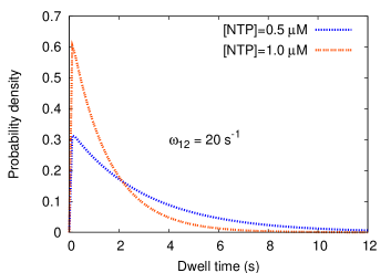
(b)

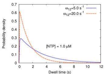
Figure 2: The dwell time distribution of a single RNAP is our model is plotted for (a) two different values of NTP concentration, keeping the rate of PP_i release (and, hence, $\omega_{12}$) fixed, and (b) two different values of $\omega_{12}$, keeping the NTP concentration fixed.

The dwell time distribution (3) is plotted in fig.2. Depending on the magnitudes of the rate constants the peak of the distribution may appear at such a small $t$ that it may not possible to detect the existence of this maxium in a laboratory experiment. In that case, the dwell time distribution would appear to be purely a single exponential adelman ; shund ; abbon . It is worth pointing out that our model does not incorporate backtracking of RNAP motors which have been observed in the in-vitro experiments shaevitz ; galburt . It has been argued by some groups neuman that short transcriptional pausing is distinct from the long pauses which arise from backtracking. In contrast, some other groups depken claim that polymerase backtracking can account for both the short and long pauses. Thus, the the role of backtracking in the pause distribution remain controversial. Moreover, it has been demonstrated that a polymerase stalled by backtracking can be re-activated by the “push” of another closely following it from behind nudler03a . Therefore, in the crowded molecular environment of intracellular space, the occurrence of backtracking may be far less frequent that those observed under in-vitro conditions. Our model, which does not allow backtracking, predicts a dwell time distribution which is qualitatively very similar to that of the short pauses provided the most probable dwell time is shorter than 1 s.

From equation (3) we get the inverse mean dwell time

$$\dfrac{1}{\langle t\rangle}=\dfrac{\tilde{V}_{max}}{1+\dfrac{\tilde{K}_{M}}{[NTP]}}$$ (6)

where $\tilde{V}_{max}=\omega_{12}$ and ${\tilde{K}_{M}}=(\omega_{12}+\omega_{12}^{b})/\tilde{\omega}^{f}_{21}$. The form of the expression (6) is identical to the Michaelis-Menten formula for the average rate of an enzymatic reaction. It describes the slowing down of the “bare” elongation progress of an RNAP due to the NTP reaction cycle that it has to undergo. The unit of velocity is $nucleotide/second$.

The fluctuations of the dwell time can be computed from the second moment

$$\langle t^{2}\rangle = \int_{0}^{\infty}~{}t^{2}~{}f(t)~{}dt$$ (7)

$$= ~{}\dfrac{2~{}\left[\left(\omega_{12}+\omega_{12}^{b}+\omega_{21}^{f}\right)^{2}~{}-~{}\omega_{12}~{}\omega_{21}^{f}\right]}{\left(\omega_{12}~{}\omega_{21}^{f}\right)^{2}}$$ (8)

of the dwell time distribution. We find the randomness parameter kou05 ; block ; ttthesis

$$\gamma = \dfrac{\langle t^{2}\rangle~{}-~{}\langle t\rangle^{2}}{\langle t\rangle^{2}}$$ (9)

$$= \dfrac{\left(\omega_{12}+\omega_{12}^{b}+\omega_{21}^{f}\right)^{2}~{}-~{}2~{}\omega_{12}~{}\omega_{21}^{f}}{\left(\omega_{12}+\omega_{12}^{b}+\omega_{21}^{f}\right)^{2}}$$ (10)

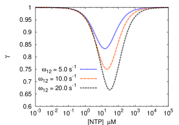
Figure 3: The randomness parameter $\gamma$ is plotted against NTP concentration for three values of the parameter $\omega_{12}$.

Note that, for a one-step Poisson process $f(t)=\omega exp(-\omega t)$, $\gamma=1$. The randomness parameter $\gamma$, given by (10), is plotted against the NTP concentration in fig.3 for three different values of $\omega_{12}$. At sufficiently low NTP concentration, $\gamma$ is unity because NTP binding with the RNAP is the rate-limiting step. As NTP concentration increases, $\gamma$ exhibits a nonmonotonic variation. At sufficiently high NTP concentration, PP_i-release (which occurs with the rate $\omega_{12}$) is the rate-limiting step and, therefore, $\gamma$ is unity also in this limit. This interpretation is consistent with the fact that the smaller is the magnitude of $\omega_{12}$, the quicker is the crossover to the value $\gamma=1$ as the NTP concentration is increased.

The randomness parameter yields the diffusion coefficient block

$$D~{}=\dfrac{\gamma}{2\langle t\rangle}$$ (11)

$$=\dfrac{\omega_{12}\omega_{21}^{f}}{\omega_{12}+\omega_{12}^{b}+\omega_{21}^{f}}\left[\dfrac{\left(\omega_{12}+\omega_{12}^{b}+\omega_{21}^{f}\right)^{2}-2\omega_{12}\omega_{21}^{f}}{2\left(\omega_{12}+\omega_{12}^{b}+\omega_{21}^{f}\right)^{2}}\right]$$

(12)

The expression (12) is in agreement with the general expression for the effective diffusion constant of a molecular motor with unbranched mechano-chemical cycle which was first reported by Fisher and Kolomeisky fishkolo .

IV Phase Diagrams

Now we will take into account the hard core steric interaction among the RNAPs which are simultaneously moving on the same DNA track. Equations (1 and 2) will be modified to

$$\frac{dP_{1}}{dt}=~{}\omega_{21}^{f}P_{2}~{}Q-~{}\omega_{12}~{}P_{1}-~{}\omega^{b}_{12}~{}P_{1}~{}Q$$ (13)

$$\frac{dP_{2}}{dt}=~{}\omega_{12}~{}P_{1}-~{}\omega_{21}^{f}~{}P_{2}~{}Q+~{}\omega_{12}^{b}~{}P_{1}~{}Q$$ (14)

Where $Q$ is conditional probability ttdc of finding site $i+\ell$ ($i-\ell-1$ for backward motion) vacant, given there is a particle at site $i$.

Due to the steric interactions between RNAP’s their stationary flux $J$ (and hence the transcription rate) is no longer limited solely by the initiation and release at the terminal sites of the template DNA. We calculate the resulting phase diagram utilizing the extremum current hypothesis (ECH) krug91 ; popkov99 . The ECH relates the flux in the system under open boundary conditions (OBC) to that under periodic boundary conditions (PBC) with the same bulk dynamics. In this approach, one imagines that initiation and termination sites are connected to two separate reservoirs where the number densities of particles are $\rho_{-}$ and $\rho_{+}$ respectively, and where the particles follow the same dynamics as in the bulk of the real physical system. Then

$$J=\left\{\begin{array}[]{ll}\mbox{max}~{}~{}j(\rho)&\mbox{if}~{}~{}\rho_{-}~{}>~{}\rho~{}>~{}\rho_{+}\\ \mbox{min}~{}~{}j(\rho)&\mbox{if}~{}~{}\rho_{-}~{}<~{}\rho~{}<~{}\rho_{+}.\end{array}\right.$$ (17)

The actual rates $\omega_{\alpha}$ and $\omega_{\beta}$ of initiation and termination of mRNA polymerization are incorporated by appropriate choice of $\rho_{-}$ and $\rho_{+}$ respectively.

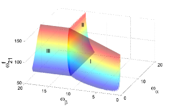
Figure 4: The 3-d phase diagram of our model for RNAP traffic. The LD and HD phases coexist on the surface $I$. The surfaces $II$ and $III$ separate the MC phase from the HD and LD phases, respectively.

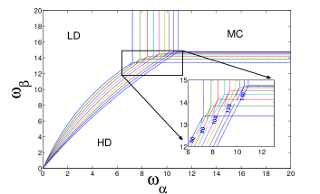
Figure 5: Projections of several 2-d phase diagram of RNAP traffic on the $\omega_{\alpha}$-$\omega_{\beta}$ plane for several values of $\omega_{21}^{f}$. The numbers on the phase boundary lines represent the value of $\omega_{21}^{f}$. The inclined lines have LD and HD above and below, respectively, while the MC phase lies in the upper right corner.

An expression for $J(\rho)$ was reported by us in Ref. ttdc . In the special case where the dominant pathway is that shown in Fig. 1 ($\omega_{12}^{b}$ = 0 for further calculation as $\omega_{12}~{}\gg~{}\omega_{12}^{b}$), we have

$$J(\rho)=\dfrac{\omega_{12}~{}\omega_{21}^{f}~{}\rho~{}(1-\rho~{}\ell)}{\omega_{12}~{}(1-\rho~{}(\ell-1))~{}+~{}\omega_{21}^{f}~{}(1-\rho~{}\ell)}$$ (19)

The number density $\rho^{*}$ that corresponds to the maximum flux is given by the expression

$$\rho^{*}=\sqrt{\dfrac{\omega_{12}~{}+~{}\omega_{21}^{f}}{\ell~{}\omega_{12}}}\left[\sqrt{\ell\left(\dfrac{\omega_{12}~{}+~{}\omega_{21}^{f}}{\omega_{12}}\right)}+1\right]^{-1}$$ (20)

By comparing (19) with the exact current-density relation of the usual TASEP for extended particles of size $\ell$ macdonald68 ; shaw03 ; Scho04 , which have no internal states (formally obtained by taking the limit $\omega_{12}\to\infty$ in the present model), we predict that the stationary current (i.e. the collective average rate of translation) is reduced by the occurrence of the intermediate state 1 through which the RNAPs have to pass.

From (17) one expects three phases, viz. a maximal-current(MC) phase with with bulk density $\rho^{*}$, a low-density phase (LD) with bulk density $\rho_{-}$, and a high-density phase (HD) with bulk density $\rho_{+}$. Using arguments similar to those used in Ref. basuchow in a similar context, we get ttthesis

$$\rho_{-}=\dfrac{\omega_{\alpha}~{}\left(\omega_{12}+\omega_{21}^{f}\right)}{\omega_{12}~{}\omega_{21}^{f}~{}+~{}\omega_{\alpha}\left(\omega_{12}+\omega_{21}^{f}\right)\left(\ell-1\right)}$$ (21)

and

$$\rho_{+}=\dfrac{\omega_{12}~{}\omega_{21}^{f}~{}-~{}\omega_{\beta}~{}\left(\omega_{12}+\omega_{21}^{f}\right)}{\omega_{12}~{}\omega_{21}^{f}~{}\ell~{}-~{}\omega_{\beta}~{}\left(\omega_{12}+\omega_{21}^{f}\right)(\ell~{}-~{}1)}.$$ (22)

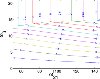
Figure 6: Same as in fig.5 except that the projections are on $\omega_{21}^{f}$-$\omega_{\beta}$ plane for several values of $\omega_{\alpha}$. The inclined lines have LD and HD above and below, respectively. Each vertical line separates the LD phase on the left from the MC phase on its right.

The condition for the coexistence of the high density (HD) and low density (LD) phases is

$$J(\rho_{-})=J(\rho_{+})$$ (23)

with $\rho_{-}<\rho^{\ast}<\rho_{+}$. Using the expression (19) for $J$ in (23) we get

$$\rho_{+} = \dfrac{\left(\omega_{12}~{}+~{}\omega_{21}^{f}\right)\left(1-\rho_{-}\ell\right)}{\ell\left(\omega_{12}~{}+~{}\omega_{21}^{f}\right)\left(1-\rho_{-}\ell\right)~{}+~{}\rho_{-}\ell\omega_{12}}.$$ (24)

Substituting (21) and (22) into (24), we get the equation for the plane of coexistence of LD and HD to be $\omega_{\beta}=f(\omega_{\alpha},\omega_{21}^{f})$ where

$$f(\omega_{\alpha},\omega_{21}^{f})=\dfrac{\left(\omega_{12}\omega_{21}^{f}\right)\omega_{12}\ell\omega_{\alpha}}{\left(\omega_{12}+\omega_{21}^{f}\right)\left[\omega_{12}\omega_{21}^{f}-\omega_{\alpha}\left(\omega_{21}^{f}+\omega_{12}-\omega_{12}\ell\right)\right]}.$$ (25)

In order to compare our result with the 2-d phase diagram of the TASEP in the $\omega_{\alpha}-\omega_{\beta}$-plane, we project 2-d cross sections of the 3-d phase diagram, for several different values of $\omega_{21}^{f}$ onto the $\omega_{\alpha}-\omega_{\beta}$-plane. The lines of coexistence of the LD and HD phases on this projected two-dimensional plane are curved , a similar curvature is also reported by Antal and Schütz antal . This is in contrast to the straight coexistence line for LD and HD phases of TASEP.

The bulk density of the system is guided by following equations:

$$\rho(\omega_{\alpha},\omega_{\beta})=\left\{\begin{array}[]{lll}\rho_{-}&~{}\mbox{if}~{}\omega_{\beta}>f(\omega_{\alpha},\omega_{21}^{f}){\rm and}~{}\omega_{\alpha}<\biggl{[}\dfrac{\rho_{*}}{1-\rho_{*}(\ell-1)}\biggr{]}\biggl{[}\dfrac{\omega_{12}\omega_{21}^{f}}{\omega_{12}+\omega_{21}^{f}}\biggr{]}~{}~{}\mbox{Low density}\\ \rho_{+}&~{}\mbox{if}~{}\omega_{\beta}<f(\omega_{\alpha},\omega_{21}^{f}){\rm and}~{}\omega_{\beta}<\biggl{[}\dfrac{1-\rho_{*}\ell}{1-\rho_{*}(\ell-1)}\biggr{]}\biggl{[}\dfrac{\omega_{12}\omega_{21}^{f}}{\omega_{12}+\omega_{21}^{f}}\biggr{]}~{}~{}\mbox{High density }\\ \rho_{*}&~{}\mbox{if}~{}\omega_{\beta}>\biggl{[}\dfrac{1-\rho_{*}\ell}{1-\rho_{*}(\ell-1)}\biggr{]}\biggl{[}\dfrac{\omega_{12}\omega_{21}^{f}}{\omega_{12}+\omega_{21}^{f}}\biggr{]}{\rm and}~{}\omega_{\alpha}>\biggl{[}\dfrac{\rho_{*}}{1-\rho_{*}(\ell-1)}\biggr{]}\biggl{[}\dfrac{\omega_{12}\omega_{21}^{f}}{\omega_{12}+\omega_{21}^{f}}\biggr{]}~{}~{}\mbox{Maximal current}.\end{array}\right.$$ (29)

In Fig. 4, we plot the 3d phase diagram.

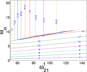
Figure 7: Same as in fig.5 except that the projections are on $\omega_{21}^{f}$-$\omega_{\alpha}$ plane for several values of $\omega_{\beta}$. Here the inclined lines have HD and LD, respectively, above and below. Each vertical line separates the HD phase on the left from the MC phase on its right.

In general, a plane $\omega^{f}_{21}$=constant intersects the surfaces I, II and III thereby generating the phase transition lines between the LD, HD and MC phases in the $\omega_{\alpha}$-$\omega_{\beta}$ plane. We have projected several of these 2d phase diagrams, each for one constant value of $\omega^{f}_{21}$ in figure 5. In the inset, we have shown the value of $\omega_{21}^{f}$ for different lines. We have also projected several 2d phase diagrams in the $\omega_{21}^{f}$-$\omega_{\beta}$ plane and $\omega_{21}^{f}$-$\omega_{\beta}$ plane, respectively, in figures 6 and 7.

V Summary and Conclusion

In this paper we have reported the exact dwell time distribution for a simple 2-state model of RNAP motors. From this distribution we have also computed the average velocity and the fluctuations of position and dwell time of RNAP’s on the DNA nucleotides. These expressions are consistent with a general formula derived earlier by Fisher and Kolomeisky for a generic model of molecular motors with unbranched mechano-chemical cycles.

Taking into account the presence of steric interactions between different RNAP moving along the same DNA template we have plotted the full 3d phase diagram of a model for multiple RNAP traffic. This model is a biologically motivated extension of the TASEP, the novel feature being the incorporation of the mechano-chemical cycle of the RNAP into the dynamics of the transcription process. This leads to a hopping process with a dwell time distribution that is not a simple exponential. Nevertheless, the phase diagram is demonstrated to follow the extremal-current hypothesis popkov99 for driven diffusive systems. Using mean field theory we have computed the effective boundary densities that enter the ECH from the reaction constants of our model. We observe that the collective average rate of translation as given by the stationary RNAP current (19) is reduced by the need of the RNAP to go through the pyrophosphate bound state. This is a prediction that is open to experimental test.

The 2d cross sections of this phase diagram have been compared and contrasted with the phase diagram for the TASEP. Unlike in the TASEP, the coexistence line between low- and high-density phase is curved for all parameter values. This is a signature of broken particle-vacancy symmetry of the RNAP dynamics. The presence of this coexistence line suggests the occurrence of RNAP “traffic jams” that our model predicts to appear when stationary initiation and release of RNAP at the terminal sites of the DNA track are able to balance each other. This traffic jam would perform an unbiased random motion, as argued earlier on general theoretical grounds in the context of protein synthesis by ribosomes from mRNA templates Schu97 .

Acknowledgments: This work is supported by a grant from CSIR (India). GMS thanks IIT Kanpur for kind hospitality and DFG for partial financial support.

References

- (1) M. Schliwa, (ed.) Molecular Motors, (Wiley-VCH, 2003).
- (2) J. Gelles and R. Landick, Cell, 93, 13 (1998).
- (3) B. Alberts et al. Essential Cell Biology, 2nd ed. (Garland Science, Taylor and Francis, 2004).
- (4) T. Tripathi and D. Chowdhury, Phys. Rev. E 77, 011921 (2008).
- (5) D. Chowdhury, L. Santen and A. Schadschneider, Phys. Rep. 329, 199 (2000).
- (6) S. Klumpp and R. Lipowsky, J. Stat. Phys. 113, 233 (2003).
- (7) D. Chowdhury, A. Schadschneider and K. Nishinari, Phys. of Life Rev. 2, 318 (2005).
- (8) M. Voliotis, N. Cohen, C. Molina-Paris and T.B. Liverpool, Biophys. J. 94, 334 (2007).
- (9) S. Klumpp and T. Hwa, PNAS 105, 18159 (2008).
- (10) G. M. Schütz, in: Phase Transitions and Critical Phenomena, vol. 19 (Acad. Press, 2001).
- (11) M. Dixon and E.C. Webb, Enzymes (Academic Press, 1979).
- (12) S.C. Kou, B.J. Cherayil, W. Min, B.P. English and X.S. Xie, J. Phys. Chem. B 109, 19068-19081 (2005).
- (13) K. Adelman, A. La Porta, T.J. Santangelo, J.T. Lis, J.W. Roberts and M.D. Wang, PNAS 99, 13538 (2002).
- (14) A. Shundrovsky, T.J. Santangelo, J.W. Roberts and M.D. Wang, Biophys. J. 87, 3945 (2004).
- (15) E.A. Abbondanzieri, W.J. Greenleaf, J.W. Shaevitz, R. Landick and S.M. Block, Nature 438, 460 (2005).
- (16) J.W. Shaevitz, E.A. Abbondanzieri, R. Landick and S.M. Block, Nature 426, 684 (2003).
- (17) E. Galburt, S.W. Grill, A. Wiedmann, L. Lubhowska, J. Choy, E. Nogales, M. Kashlev and C. Bustamante, Nature 446, 820 (2007).
- (18) K.C. Neuman, E.A. Abbondanzieri, R. Landick, J. Gelles and S.M. Block, Cell 115, 437 (2003).
- (19) M. Depken, E. Galburt and S.W. Grill, Biophys. J. 96, 2189 (2009).
- (20) V. Epshtein and E. Nudler, Science 300, 801 (2003).
- (21) M. Schnitzer and S. Block, Cold Spring Harbor Symp. Quant. Biol. 60, 793 (1995)
- (22) T. Tripathi, Ph.D. thesis, IIT Kanpur (2009).
- (23) M.E. Fisher and A.B. Kolomeisky, PNAS 96, 6597 (1999).
- (24) V. Popkov and G. M. Schütz, Europhys. Lett. 48, 257 (1999).
- (25) J. Krug, Phys. Rev. Lett. 67, 1882 (1991).
- (26) C. MacDonald, J. Gibbs and A. Pipkin, Biopolymers, 6, 1 (1968).
- (27) L.B. Shaw, R.K.P. Zia and K.H. Lee, Phys. Rev. E 68, 021910 (2003).
- (28) G. Schönherr and G.M. Schütz, J. Phys. A 37, 8215 (2004).
- (29) A. Basu and D. Chowdhury, Phys. Rev. E 75, 021902 (2007).
- (30) T. Antal and G. M. Schütz, Phys. Rev. E 62, 83 (2000).
- (31) G.M. Schütz, Int. J. Mod. Phys. B 11, 197 (1997).