Discrete Geometric Structures in Homogenization and Inverse Homogenization with application to EIT.

Abstract

We introduce a new geometric approach for the homogenization and inverse homogenization of the divergence form elliptic operator with rough conductivity coefficients $\sigma(x)$ in dimension two. We show that conductivity coefficients are in one-to-one correspondence with divergence-free matrices and convex functions $s(x)$ over the domain $\Omega$. Although homogenization is a non-linear and non-injective operator when applied directly to conductivity coefficients, homogenization becomes a linear interpolation operator over triangulations of $\Omega$ when re-expressed using convex functions, and is a volume averaging operator when re-expressed with divergence-free matrices. We explicitly give the transformations which map conductivity coefficients into divergence-free matrices and convex functions, as well as their respective inverses. Using optimal weighted Delaunay triangulations for linearly interpolating convex functions, we apply this geometric framework to obtain an optimally robust homogenization algorithm for arbitrary rough coefficients, extending the global optimality of Delaunay triangulations with respect to a discrete Dirichlet energy to weighted Delaunay triangulations. Next, we consider inverse homogenization, that is, the recovery of the microstructure from macroscopic information, a problem which is known to be both non-linear and severly ill-posed. We show how to decompose this reconstruction into a linear ill-posed problem and a well-posed non-linear problem. We apply this new geometric approach to Electrical Impedance Tomography (EIT) in dimension two. It is known that the EIT problem admits at most one isotropic solution. If an isotropic solution exists, we show how to compute it from any conductivity having the same boundary Dirichlet-to-Neumann map. This is of practical importance since the EIT problem always admits a unique solution in the space of divergence-free matrices and is stable with respect to $G$-convergence in that space (this property fails for isotropic matrices). As such, we suggest that the space of convex functions is the natural space to use to parameterize solutions of the EIT problem.

1 Introduction

In this paper, we introduce a new geometric framework of the homogenization and inverse homogenization of the divergence-form elliptic operator

$$u\rightarrow-\operatorname{div}(\sigma\nabla u)$$ (1.1)

where $\sigma$ is symmetric, uniformly elliptic and with entries $\sigma_{ij}\in L^{\infty}$. Owing to its physical interpretation, we refer to $\sigma$ as the conductivity.

The classical theory of homogenization is based on abstract operator convergence and deals with the asymptotic limit of a sequence of operators of the form (1.1) parameterized by a small parameter $\epsilon$. We refer to $G$-convergence for symmetric operators, $H$-convergence for non-symmetric operators and $\Gamma$-convergence for variational problems [61, 40, 33, 75, 74, 63, 25]. We also refer to [18] for the original formulation based on asymptotic analysis and [48] for a review.

Instead of considering the homogenized limit of an $\epsilon$-family of operators of the form (1.1), we will construct in this paper a sequence of finite dimensional and low rank operators approximating (1.1) with arbitrary bounded $\sigma(x)$. More precisely, since no small parameter $\epsilon$ is introduced in the formulation, one has to understand homogenization in the context of finite dimensional approximation using a parameter $h$ that represents a computational scale determined by the available computational power and the desired precision. We are motivated by the fact that in most engineering problems, one has to deal with a given medium and not with an $\epsilon$-family of media.

This observation gave rise to methods such as special finite element methods, metric based upscaling and harmonic change of coordinates considered in [15, 16, 68, 69, 67, 55, 19]. This point of view recovers not only results from classical homogenization with periodic or ergodic coefficients but also allows for homogenization of a given medium with arbitrary rough coefficients. In particular we need not make assumptions of ergodicity, scale separation and we do not need to introduce small parameter $\epsilon$.

Our formalism, in not relying on small parameter $\epsilon$, is closely related to numerical homogenization which deals with coarse scale numerical approximations of solutions of (2.1) below. Here we refer to the subspace projection formalism [65], the multiscale finite element method [45], the mixed multiscale finite element method [12], the heterogeneous multiscale method [36, 39], sparse chaos approximations [80, 44]; finite difference approximations based on viscosity solutions [27], operator splitting methods [13] and generalized finite element methods [76]. We refer to [38, 37] for an numerical implementation of the idea of a global change of harmonic coordinates for porous media and reservoir modeling.

Contributions.

In this paper, we focus on the intrinsic geometric framework underlying homogenization. First we show that conductivities $\sigma$ can be put into one-to-one correspondence with, that is, can be parameterized by, symmetric definite positive divergence free matrices $Q$, and by convex functions $s$ as well (Section 2.2). While the transformation which maps $\sigma$ into effective conductivities $q^{h}$ per coarse edge element is a highly non-linear transformation (Section 2.1), we show that homogenization in the space of symmetric definite positive divergence free matrices $Q$ acts as volume averaging, and hence is linear, while homogenization in the space of convex functions $s$ acts as a linear interpolation operator (Section 3). Moreover, we show that homogenization as it is formulated here is self-consistent and satisfies a semi-group property (Section 3.3).

Hence, once formulated in the proper space, homogenization is a linear interpolation operator acting on convex functions. We apply this observation to construct optimally robust and stable algorithms for homogenizing divergence form equations with arbitrary rough coefficients by using weighted Delaunay triangulations for linearly interpolating convex functions (Section 4). Figure 1.1 summarizes relationships between the different parameterizations for conductivity we study.

   

Figure 1.1: Relationships between parameterizations of conductivity. Straight and wavy lines represent linear and non-linear relationships, respectively.

We use this new geometric framework for reducing the complexity of an inverse homogenization problem (Section 5). Inverse homogenization deals with the recovery of the physical conductivity $\sigma$ from coarse scale information, for instance, from the set of effective conductivities. This problem is ill-posed insofar as it has no unique solution, and the space of solutions is a highly nonlinear manifold. We use this new geometric framework to re-cast inverse homogenization into an optimization problem within a linear space.

We apply this result to Electrical Impedance Tomography (EIT), the problem of computing $\sigma$ from Dirichlet and Neumann data measured on the boundary of our domain. First, we provide a new method for solving EIT problems through parameterization via convex functions. Next we use this new geometric framework to obtain new theoretical results on the EIT problem (Section 6). Although the EIT problem admits at most one isotropic solution, this isotropic solution may not exist if the boundary data have been measured on an anisotropic medium. We show that the EIT problem admits a unique solution in the space of divergence-free matrices. The uniqueness property has also been obtained in [5]. When conductivities are endowed with the topology of $G$-convergence the inverse conductivity problem is discontinuous when restricted to isotropic matrices [53, 5] and continuous when restricted to divergence-free matrices [5].

If an isotropic solution exists we show here how to compute it for any conductivity having the same boundary data. This is of practical importance since the medium to be recovered in a real application may not be isotropic and the associated EIT problem may not admit an isotropic solution but if such an isotropic solution exists it can be computed from the divergence-free solution by solving PDE (6.6).

As such, we suggest that the space of divergence-free matrices parametrized by the space of convex functions is the natural space to look into for solutions of the EIT problem.

2 Homogenization and parametrization of the conductivity space.

To illustrate our new approach, we will consider, as a first example, the homogenization of the Dirichlet problem

$$\left\{\begin{aligned} -\operatorname{div}\left(\sigma\nabla u\right)&=f,\enspace&x\in\Omega,\\ u&=0,\enspace&x\in\partial\Omega.\end{aligned}\right.$$ (2.1)

$\Omega$ is a bounded convex subset of $\mathbb{R}^{d}$ with a $C^{2}$ boundary, and $f\in L^{\infty}(\Omega)$. The condition on $f$ can be relaxed to $f\in L^{2}(\Omega)$, but for the sake of simplicity we will restrict our presentation to $f\in L^{\infty}(\Omega)$.

Let $F:\Omega\rightarrow\Omega$ denote the harmonic coordinates associated with (2.1). That is, $F(x)=\big{(}F_{1}(x),\ldots,F_{d}(x)\big{)}$ is a $d$-dimensional vector field whose coordinates satisfy

$$\left\{\begin{aligned} \operatorname{div}\left(\sigma\nabla F_{i}\right)&=0,\enspace&x\in\Omega,\\ F_{i}(x)&=x_{i},\enspace&x\in\partial\Omega.\end{aligned}\right.$$ (2.2)

In dimension $d=2$ it is known that $F$ is a homeomorphism from $\Omega$ onto $\Omega$ and $\det(\nabla F)>0$ a.e. [10, 6, 11]. For $d\geq 3$, $F$ may be non-injective, even if $\sigma$ is smooth [10, 11, 26]. We will restrict our presentation to $d=2$.

For a given symmetric matrix $M$, we denote by $\lambda_{\max}(M)$ and $\lambda_{\min}(M)$ its maximal and minimal eigenvalues. Define

$$\mu:=\Big{\|}\frac{\lambda_{\max}((\nabla F)^{T}\nabla F)}{\lambda_{\min}((\nabla F)^{T}\nabla F)}\Big{\|}_{L^{\infty}(\Omega)}.$$ (2.3)

We will call condition (2.4) the following non-degeneracy condition on the anisotropy of $(\nabla F)^{T}\nabla F$

$$\mu<\infty.$$ (2.4)

For $d=2$, (2.4) is always satisfied if $\sigma$ is smooth [6] or even Hölder continuous [11].

2.1 Homogenization as a non-linear operator

Let $\Omega_{h}$ be a regular triangulation of $\Omega$ having resolution $h$. Let $X_{h}$ be the set of piecewise linear functions on $\Omega_{h}$ with Dirichlet boundary conditions. Let $\mathcal{N}_{h}$ be the set of interior nodes of $\Omega_{h}$. For each node $i\in\mathcal{N}_{h}$, denote $\varphi_{i}$ the piecewise linear nodal basis functions equal to $1$ on the node $i$ and $0$ on the other nodes. Let $\mathcal{E}_{h}$ be the set of interior edges of $\Omega_{h}$, hence if $e\in\mathcal{E}_{h}$ then $e=(i,j)$ where $i$ and $j$ are distinct interior nodes and share the edge of two triangles of $\Omega_{h}$.

2.1 Definition (Effective edge conductivities).

Let $q^{h}$ be the mapping from $\mathcal{E}_{h}$ onto $\mathbb{R}$, such that for $(i,j)\in\mathcal{E}_{h}$

$$q_{ij}^{h}:=-\int_{\Omega}(\nabla(\varphi_{i}\circ F))^{T}\sigma(x)\nabla(\varphi_{j}\circ F)\,dx.$$ (2.5)

Observe that $q_{ij}^{h}=q_{ji}^{h}$, hence $q^{h}$ is only a function of undirected edges $(i,j)$. We refer to $q_{ij}^{h}$ as the effective conductivity of the edge $(i,j)$.

Let $\mathcal{M}$ be the space of $2\times 2$ uniformly elliptic, bounded and symmetric matrix fields on $\Omega$. Let $T_{q^{h},\sigma}$ be the operator mapping $\sigma$ onto $q^{h}$ defined by (2.5). Let $\mathcal{Q}_{h}$ be the image of $T_{q^{h},\sigma}$.

$$\begin{split}T_{q^{h},\sigma}\,:\,\mathcal{M}&\longrightarrow\mathcal{Q}_{h}\\ \sigma&\longrightarrow T_{q^{h},\sigma}[\sigma]:=q^{h}.\end{split}$$ (2.6)

Observe that $T_{q^{h},\sigma}$ is both non-linear and non-injective.

Let $j\sim i$ be the set of interior nodes $j$, distinct from $i$, that share an edge with $i$.

2.2 Definition (Homogenized problem).

Consider the vector $(u^{h}_{i})_{i\in\mathcal{N}_{h}}$ of $\mathbb{R}^{\mathcal{N}_{h}}$ such that for all $i\in\mathcal{N}_{h}$,

$$\sum_{j\sim i}q_{ij}^{h}(u^{h}_{i}-u^{h}_{j})=\int_{\Omega}f(x)\varphi_{i}\circ F(x)\,dx.$$ (2.7)

We refer to this finite difference problem for $(u^{h}_{i})_{i\in\mathcal{N}_{h}}$ associated to $q^{h}$ as the homogenized problem.

The identification of effective edge conductivities and the homogenized problem is motivated by the following theorem:

2.3 Theorem.

The homogenized problem (2.7) has a solution $(u^{h}_{i})_{i\in\mathcal{N}_{h}}$ and it is unique. Moreover, let $u$ be the solution of (2.1) and define

$$u_{h}:=\sum_{i\in\mathcal{N}_{h}}u_{i}^{h}\varphi_{i}\circ F.$$ (2.8)

If condition (2.4) holds, then

$$\|u-u_{h}\|_{H^{1}_{0}(\Omega)}\leq Ch\|f\|_{L^{\infty}(\Omega)}.$$ (2.9)

2.4 Remark.

We refer to [68] and [69] for numerical results associated with theorem 2.3.

2.5 Remark.

The constant $C$ depends on $\|1/\lambda_{\min}(\sigma)\|_{L^{\infty}(\Omega)}$, $\|\lambda_{\max}(\sigma)\|_{L^{\infty}(\Omega)}$, $\Omega$, and $\mu$. Replacing $\|f\|_{L^{\infty}(\Omega)}$ by $\|f\|_{L^{2}(\Omega)}$ in (2.9) adds a dependence of $C$ on $\big{\|}(\det(\nabla F))^{-1}\big{\|}_{L^{\infty}(\Omega)}$.

2.6 Remark.

Although the proof of the theorem shows a dependence of $C$ on $\mu$ associated with condition (2.4), numerical results in dimension two indicate that $C$ is mainly correlated with the contrast (minimal and maximal eigenvalues) of $a$. This is why we believe that there should be a way of proving (2.3) without condition (2.4). We refer to sections 2 and 3 of [6] for the detailed analysis of a similar condition (definition 2.1 of [6]).

2.7 Remark.

Problem (2.7) and Theorem 2.3 represent an generalization of method I of [16] to non-laminar media (see also [68]).

2.8 Remark.

It is also proven in [68] (proof of Theorem 1.14) that if $f\in L^{\infty}(\Omega)$ then there exist constants $C,\alpha>0$ such that $u\circ F^{-1}\in C^{1,\alpha}(\Omega)$ and

$$\|\nabla(u\circ F^{-1})\|_{C^{\alpha}(\Omega)}\leq C\|f\|_{L^{\infty}(\Omega)},$$ (2.10)

where constants $C$ and $\alpha$ depend on $\Omega$, $\|1/\lambda_{\min}(\sigma)\|_{L^{\infty}(\Omega)}$, $\|\lambda_{\max}(\sigma)\|_{L^{\infty}(\Omega)}$, and $\mu$. We also refer to [16] (for quasi-laminar media) and [6] for similar observations (on connections with quasi-regular and quasi-conformal mappings)

2.9 Remark.

Unlike a canonical finite element treatment, where we consider only approximation of the solution, here we are also considering approximation of the operator. This consideration is important, for example, in multi-grid solvers which rely on a set of operators which are self-consistent over a range of scales.

Proof of Theorem 2.3.

The proof is similar to the proofs of Theorems 1.16 and 1.23 of [68]; we also refer to [19]. For the sake of completeness we will recall its main lines.

Write $Q$ the matrix (2.24). Replacing $u$ by $\hat{u}\circ F$ in (2.1) we obtain after differentiation and change of variables that $\hat{u}:=u\circ F^{-1}$ satisfies

$$\left\{\begin{aligned} -\sum_{i,j}Q_{ij}\partial_{i}\partial_{j}\hat{u}&=\frac{f}{\det(\nabla F)}\circ F^{-1},\enspace&x\in\Omega,\\ u&=0,\enspace&x\in\partial\Omega.\end{aligned}\right.$$ (2.11)

Similarly, multiplying (2.1) by test functions $\varphi\circ F$ (with $\varphi$ satisfying a Dirichlet boundary condition), integrating by parts and using the change variables $y=F(x)$ we obtain that

$$\int_{\Omega}(\nabla\varphi)^{T}Q\nabla\hat{u}=\int_{\Omega}\varphi\frac{f}{\det(\nabla F)}\circ F^{-1}.$$ (2.12)

Observing that $\hat{u}$ satisfies the non-divergence form equation, we obtain, using Theorems 1.2.1 and 1.2.3 of [59], that if $Q$ is uniformly elliptic and bounded, then $\hat{u}\in W^{2,2}(\Omega)$ with

$$\|\hat{u}\|_{W^{2,2}(\Omega)}\leq C\|f\|_{L^{\infty}(\Omega)}.$$ (2.13)

The constant $C$ depends on $\Omega$ and bounds on the minimal and maximal eigenvalues of $Q$. We have used the fact that the Cordes-type condition on $Q$ required by [59] simplifies for $d=2$.

Next, let $V_{h}$ be the linear space defined by $\varphi\circ F$ for $\varphi\in X_{h}$. Write $u_{h}$ the finite element solution of (2.1) in $V_{h}$. Writing $u_{h}$ as in (2.8) we obtain that the resulting finite-element linear system can be written as

$$-q_{ii}^{h}u^{h}_{i}-\sum_{j\sim i}q_{ij}^{h}u^{h}_{j}=\int_{\Omega}f(x)\varphi_{i}\circ F(x)\,dx,$$ (2.14)

for $i\in\mathcal{N}_{h}$. We use definition (2.5) for $q_{ij}^{h}$. Using the change of variables $y=F(x)$ we obtain that $q_{ij}^{h}$ can be written

$$q_{ij}^{h}:=-\int_{\Omega}(\nabla\varphi_{i})^{T}Q(x)\nabla\varphi_{j}\,dx.$$ (2.15)

Decomposing the constant function $1$ over the basis $\varphi_{j}$ we obtain that

$$-\int_{\Omega}(\nabla\varphi_{i})^{T}Q(x).\nabla(\sum_{j}\varphi_{j})\,dx=0,$$ (2.16)

from which we deduce that

$$q_{ii}^{h}+\sum_{j\sim i}q_{ij}^{h}=0.$$ (2.17)

Combining (2.17) with (2.14) we obtain that the vector $(u^{h}_{i})_{i\in\mathcal{N}_{h}}$ satisfies equation (2.7).

Using the change of variables $y=F(x)$ in

$$\int_{\Omega}(\nabla(\varphi_{i}\circ F))^{T}\sigma(x).\nabla u_{h}\,dx=\int_{\Omega}\varphi_{i}\circ F\,f,$$ (2.18)

we obtain that $\hat{u}_{h}:=u_{h}\circ F^{-1}$ satisfies

$$\int_{\Omega}(\nabla\varphi_{i})^{T}Q\nabla\hat{u}_{h}=\int_{\Omega}\varphi_{i}\frac{f}{\det(\nabla F)}\circ F^{-1}.$$ (2.19)

Hence $\hat{u}_{h}$ is the finite element approximation of $\hat{u}$. Using the notation $\sigma[v]:=\int_{\Omega}\nabla v^{T}\sigma\nabla v$ we obtain through the change of variables $y=F(x)$ that $\sigma[v]=Q[v\circ F^{-1}]$. It follows that

$$\sigma[u-u_{h}]=Q[\hat{u}-\hat{u}_{h}].$$ (2.20)

Since $\hat{u}_{h}$ minimizes $Q[\hat{u}-v]$ over $v\in X_{h}$ we obtain equation (2.9) from the $W^{2,2}$-regularity of $\hat{u}$ (2.13). ∎

The fact that $q^{h}$, as a quadratic form on $\mathbb{R}^{\mathcal{N}_{h}}$, is positive definite can be obtained from the following proposition:

2.10 Proposition.

For all vectors $(v_{i})_{i\in\mathcal{N}_{h}}\in\mathbb{R}^{\mathcal{N}_{h}}$,

$$\sum_{i\sim j}v_{i}q_{ij}^{h}v_{j}=\int_{\Omega}(\nabla(v\circ F))^{T}\sigma\nabla(v\circ F),$$ (2.21)

where $v:=\sum_{i\in\mathcal{N}_{h}}v_{i}\;\varphi_{i}$.

Proof.

The proof follows from first observing that

$$\sum_{i\sim j}v_{i}q_{ij}^{h}v_{j}=\int_{\Omega}(\nabla v)^{T}(y)Q(y)(\nabla v)(y)\,dy,$$ (2.22)

then applying the change of variables $y=F(x)$. ∎

2.11 Remark.

Despite the fact that positivity holds for any triangulation $\Omega_{h}$, as we shall examine in Section 4, we can take advantage of the freedom to choose $\Omega_{h}$ to produce $q_{ij}^{h}$ which give linear systems representing homogenized problems (2.7) having optimal conditioning properties.

2.2 Parametrization of the conductivity space

We now take advantage of special properties of $\sigma$ when transformed by its harmonic coordinates $Q$ to parameterize the space of conductivities.

2.12 Definition (Space of divergence-free matrices).

We say that a matrix field $M$ on $\Omega$ is divergence-free if its columns are divergence-free vector fields. That is, $M$ is divergence-free if for all $v\in C^{\infty}_{0}$ and $l\in\mathbb{R}^{2}$

$$\int_{\Omega}(\nabla v)^{T}\,M.l=0$$ (2.23)

2.13 Definition (Divergence-free conductivity).

Given the conductivity $\sigma$ associated to (1.1) and a domain $\Omega$, define $Q$ to be the symmetric $2\times 2$ matrix given by

$$Q=F_{\ast}\sigma:=\frac{(\nabla F)^{T}\sigma\nabla F}{\det(\nabla F)}\circ F^{-1}.$$ (2.24)

Again, $F:\Omega\rightarrow\Omega$ are the harmonic coordinates (2.2) associated to $\sigma$.

2.14 Proposition (Properties of $Q$).

$Q$ satisfies the following properties:

• $Q$ is positive-definite, symmetric and divergence-free.

• $Q\in(L^{1}(\Omega))^{d\times d}$.

• $\det(Q)$ is uniformly bounded away from $0$ and $\infty$.

• $Q$ is bounded and uniformly elliptic if and only if $\sigma$ satisfies the non-degeneracy condition (2.4).

Proof.

Equations (2.11) and (2.12) imply that for all $\hat{u}\in H^{1}_{0}\cap H^{2}(\Omega)$ and all $\varphi\in C^{\infty}_{0}(\Omega)$

$$\int_{\Omega}(\nabla\varphi)^{T}Q\nabla\hat{u}=-\int_{\Omega}\varphi\sum_{i,j}Q_{ij}\partial_{i}\partial_{j}\hat{u}.$$ (2.25)

Let $l\in\mathbb{R}^{d}$, choosing $\hat{u}$ such that $\nabla\hat{u}=l$ on the support of $\varphi$ we obtain that for all $l\in\mathbb{R}^{d}$

$$\int_{\Omega}(\nabla\varphi)^{T}Q\cdot l=0$$ (2.26)

It follows by integration by parts that $\operatorname{div}(Q\cdot l)=0$ in the weak sense and hence $Q$ is divergence-free (its columns are divergence-free vector fields, this has also been obtained in [68]). The second and third part of the Proposition can be obtained from

$$\det(Q)=\det\big{(}\sigma\circ F^{-1}\big{)},$$ (2.27)

and

$$\int_{\Omega}Q=\int_{\Omega}(\nabla F)^{T}\sigma\nabla F$$ (2.28)

The last part of the Proposition can be obtained from the following inequalities (valid for $d=2$). For $x\in\Omega$ a.e.,

$$\lambda_{\max}(Q)\leq\lambda_{\max}(\sigma)\sqrt{\frac{\lambda_{\max}((\nabla F)^{T}\nabla F)}{\lambda_{\min}((\nabla F)^{T}\nabla F)}}$$ (2.29)

$$\lambda_{\min}(Q)\geq\lambda_{\min}(\sigma)\sqrt{\frac{\lambda_{\min}((\nabla F)^{T}\nabla F)}{\lambda_{\max}((\nabla F)^{T}\nabla F)}}$$ (2.30)

∎

Write $T_{Q,\sigma}$ the operator mapping $\sigma$ onto $Q$ through equation (2.24). That is,

$$\begin{split}T_{Q,\sigma}\,:\,\mathcal{M}&\longrightarrow\mathcal{M}_{\operatorname{div}}\\ M&\longrightarrow T_{Q,\sigma}[M]:=\frac{(\nabla F_{M})^{T}M\nabla F_{M}}{\det(\nabla F_{M})}\circ F^{-1}_{M},\end{split}$$ (2.31)

where $F_{M}$ are the harmonic coordinates associated to $M$ through equation (2.2) (for $\sigma\equiv M$) and $\mathcal{M}_{\operatorname{div}}$ is the image of $\mathcal{M}$ under the operator $T_{Q,\sigma}$. Observe (from Proposition 2.14) that $\mathcal{M}_{\operatorname{div}}$ is a space of $2\times 2$ of symmetric, positive and divergence-free matrix fields on $\Omega$, with entries in $L^{1}(\Omega)$ and with determinants uniformly bounded away from $0$ and infinity.

Since for all $M\in\mathcal{M}_{\operatorname{div}}$, $T_{Q,\sigma}[M]=M$ ($T_{Q,\sigma}$ is a non-linear projection onto $\mathcal{M}_{\operatorname{div}}$) it follows that $T_{Q,\sigma}$ is a non-injective operator from $\mathcal{M}$ onto $\mathcal{M}_{\operatorname{div}}$. Now denote $\mathcal{M}_{\operatorname{iso}}$ the space of $2\times 2$ isotropic, uniformly elliptic, bounded and symmetric matrix fields on $\Omega$. Hence matrices in $\mathcal{M}_{\operatorname{iso}}$ are of the form $\sigma(x)I_{d}$ where $I_{d}$ is the $d\times d$ identity matrix and $\sigma(x)$ is a scalar function.

2.15 Theorem.

The following statements hold in dimension $d=2$:

1. The operator $T_{Q,\sigma}$ is an injection from $\mathcal{M}_{\operatorname{iso}}$ onto $\mathcal{M}_{\operatorname{div}}$.

2. $$T_{Q,\sigma}^{-1}[Q]=\sqrt{\det(Q)\circ G^{-1}}\,I_{d},$$ (2.32)

   where $G$ are the harmonic coordinates associated to $\frac{Q}{\sqrt{\det(Q)}}$. That is, $G_{i}(x),i=1,2$ is the unique solution of

   $$\left\{\begin{aligned} \operatorname{div}\left(\frac{Q}{\sqrt{\det(Q)}}\nabla G_{i}\right)&=0\enspace&x\in\Omega,\\ G_{i}(x)&=x_{i}\enspace&x\in\partial\Omega.\end{aligned}\right.$$ (2.33)

3. $G=F^{-1}$ where $G$ is the transformation defined by (2.33), and $F$ are the harmonic coordinates associated to $\sigma:=T_{Q,\sigma}^{-1}[Q]$ by (2.2).

2.16 Remark.

Observe that the non degeneracy condition (2.4) is not necessary for the validity of this theorem.

2.17 Remark.

$T_{Q,\sigma}$ is not surjective from $\mathcal{M}_{\operatorname{iso}}$ onto $\mathcal{M}_{\operatorname{div}}$. This can be proven by contradiction by assuming $Q$ to be a non-isotropic constant matrix. Constant $Q$ is trivially divergence-free, yet it follows that $\sigma=\sqrt{\det(Q)}I_{d}$, $F(x)=x$ and $Q$ is isotropic, which is a contradiction.

2.18 Remark.

$T_{Q,\sigma}$ is not an injection from $\mathcal{M}$ onto $\mathcal{M}_{\operatorname{div}}$ . However it is known [60] that for each $\sigma\in\mathcal{M}$ there exists a sequence $\sigma_{\epsilon}$ in $\mathcal{M}_{\operatorname{iso}}$ $H$-converging towards $\sigma$. (Moreover, this sequence can be chosen to be of the form $a(x,x/\epsilon)$, where $a(x,y)$ is periodic in $y$.) Since $\mathcal{M}_{\operatorname{iso}}$ is dense in $\mathcal{M}$ with respect to the topology induced by $H$-convergence, and since $T_{Q,\sigma}$ is an injection from $\mathcal{M}_{\operatorname{iso}}$, the scope of applications associated with the existence of $T_{Q,\sigma}^{-1}$ would not suffer from a restriction from $\mathcal{M}$ to $\mathcal{M}_{\operatorname{iso}}$.

Proof of Theorem 2.15.

First observe that if $\sigma$ is scalar then we obtain from equation (2.24) that

$$\det(Q)=\big{(}\sigma\circ F^{-1}\big{)}^{2},$$ (2.34)

and hence

$$\sigma=\sqrt{\det(Q)\circ F}.$$ (2.35)

Consider again equation (2.24). Let $R$ be the $2\times 2$, $\frac{\pi}{2}-$rotation matrix in $\mathbb{R}^{2}$, that is,

$$R=\begin{pmatrix}0&-1\\ 1&0\end{pmatrix}.$$ (2.36)

Observe that for a $2\times 2$ matrix $A$,

$$(A^{-1})^{T}=\frac{1}{\det(A)}R\,A\,R^{T}.$$ (2.37)

Write $G:=F^{-1}$. Recall that

$$\nabla G=(\nabla F)^{-1}\circ F^{-1}.$$ (2.38)

Applying (2.38) to (2.24) gives

$$Q\nabla G=\det(\nabla G)((\nabla G)^{-1})^{T}\sigma\circ G.$$ (2.39)

Using $\sqrt{\det(Q)}=\sigma\circ G$ and applying equation (2.37) to $((\nabla G)^{-1})^{T}$ we obtain that

$$\frac{Q}{\sqrt{\det(Q)}}\nabla G=R\;\nabla G\;R^{T}.$$ (2.40)

Observing that in dimension two, for all functions $v\in H^{1}$, $\operatorname{div}(R\nabla v)=0$, and we obtain from (2.40) that $G$ satisfies equation (2.33). The boundary condition comes from the fact that $G=F^{-1}$, where $F$ is a diffeomorphism and $F(x)=x$ on $\partial\Omega$. Let us now show that equation (2.33) admits a unique solution. If $G_{i}^{\prime}$ is another solution of equation (2.33) then

$$\nabla(G_{i}-G_{i}^{\prime})\frac{Q}{\sqrt{\det(Q)}}\nabla(G_{i}-G_{i}^{\prime})=0$$ (2.41)

Since $Q$ is positive with $L^{1}$ entries and $\det(Q)$ is uniformly bounded away from zero and infinity it follows that $\frac{Q}{\sqrt{\det(Q)}}$ is positive and its minimal eigenvalue is bounded away from infinity almost everywhere in $\Omega$. It follows that $\nabla(G_{i}-G_{i}^{\prime})=0$ almost everywhere in $\Omega$ and we conclude from the boundary condition on $G_{i}$ and $G_{i}^{\prime}$ that $G_{i}=G_{i}^{\prime}$ almost everywhere in $\Omega$. ∎

2.19 Definition (The space of convex functions).

Consider the space of $W^{2,1}(\Omega)$ convex functions on $\Omega$ whose discriminants (determinant of the Hessian) are uniformly bounded away from zero and infinity. Write $\mathcal{S}$ the quotient set on that space defined by the equivalence relation: $s\sim s^{\prime}$ if $s-s^{\prime}$ is an affine function. Let $R$ be the rotation matrix (2.36).

2.20 Theorem (Scalar parameterization of conductivity in $\mathbb{R}^{2}$).

For each $Q\in\mathcal{M}_{\operatorname{div}}$ there exists a unique $s\in\mathcal{S}$ such that

$$\operatorname{Hess}(s)=R^{T}QR,$$ (2.42)

where $\operatorname{Hess}(s)$ is the Hessian of $s$.

2.21 Remark.

Since $Q$ is positive-definite one concludes that $\operatorname{Hess}(s)$ is positive-definite, and thus, $s(x)$ is convex. Furthermore, the principal curvature directions of $s(x)$ are the eigenvectors of $Q$, rotated by $\pi/2$. Note that this geometric characteristic will be crucial later when we approximate $s(x)$ by piecewise-linear polynomials, which are not everywhere differentiable—but for which the notion of convexity is still well defined.

Proof.

In $\mathbb{R}^{2}$, the symmetry and divergence-free constraints on $Q$ reduce the number of degrees of freedom of $Q(x)$ to a single one. This remaining degree of freedom is $s(x)$, our scalar convex parameterizing function. To construct $s(x)$, observe that as a consequence of the Hodge decomposition, there exist functions $h,k\in W^{1,1}(\Omega)$ such that

$$Q=\begin{pmatrix}a&b\\ b&c\end{pmatrix}=\begin{pmatrix}h_{y}&k_{y}\\ -h_{x}&-k_{x}\end{pmatrix}$$ (2.43)

where $a,b,c$ are scalar functions. These choices ensure that the divergence-free condition is satisfied, namely that $a_{x}+b_{y}=b_{x}+c_{y}=0$. Another application of the Hodge decomposition gives the existence of $s\in W^{2,1}(\Omega)$ such that $\nabla s=\left(-k,h\right)^{T}$. This choice ensures that $b=-h_{x}=k_{y}=-s_{xy}$, the symmetry condition. The functions $h$ and $k$ are unique up to the addition of arbitrary constants, so $s$ is unique up to the addition of affine functions of the type $\alpha x+\beta y+\gamma$, where $\alpha,\beta,\gamma\in\mathbb{R}$ are arbitrary constants. ∎

We write $T_{s,Q}$ the operator from $\mathcal{M}_{\operatorname{div}}$ onto $\mathcal{S}$ mapping $Q$ onto $s$. Observe that

$$\begin{split}T_{s,Q}\,:\,\mathcal{M}_{\operatorname{div}}&\longrightarrow\mathcal{S}\\ Q&\longrightarrow T_{s,Q}[Q]=s\end{split}$$ (2.44)

is a bijection and

$$T_{s,Q}^{-1}[s]=R\operatorname{Hess}(s)R^{T}.$$ (2.45)

Refer to Figure 2.1 for a summary of the relationships between $\sigma$, $Q$ and $s$. Figures 2.2 and 2.3 show an example conductivity in each of the three spaces.

Figure 2.1: The three parameterizations of conductivity, and the spaces to which each belongs.

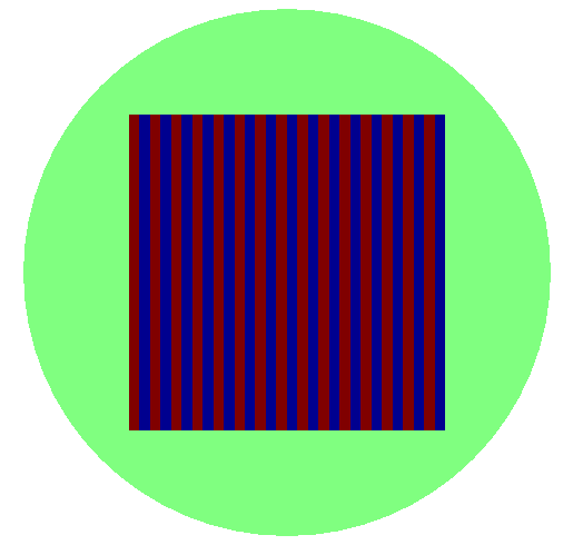
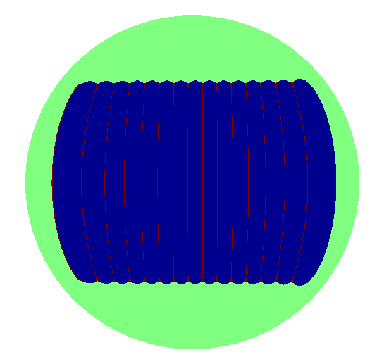
Figure 2.2: The left-hand image shows the original scalar conductivity $\sigma(x)=a(x)\operatorname{Id}$. In blue regions a=0.05, in red regions a=1.95, and in green regions, a = 1.0. The right-hand image gives $\sqrt{\det(Q)}=\sigma\circ F^{-1}$, showing how harmonic coordinates distort $\sigma(x)$.

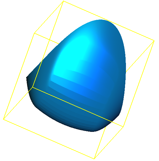
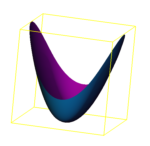
Figure 2.3: Two views of the fine-scale function $s(x)$ represented as a height field surface for the laminated conductivity of Figure 2.2. The left-hand view shows the fine-scale pattern in $\sigma(x)$, and the right-hand view highlights the coarse-scale anisotropy in the curvature.

3 Discrete geometric homogenization

We now apply the results of Section 2 to show that in our framework, homogenization can be represented either as volume averaging, or as interpolation. Thus, unlike direct homogenization of $\sigma\in\mathcal{M}$, homogenization in $\mathcal{M}_{\operatorname{div}}$ or $\mathcal{S}$ is a linear operation. Moreover, in this framework, homogenization inherits the semi-group property enjoyed by volume averaging and interpolation, giving a self-consistency to homogenization in our setting.

3.1 Homogenization by volume averaging

The operator $T_{q^{h},\sigma}$ defined in (2.6) is a non-linear operator on $\mathcal{M}$. However, its restriction to $\mathcal{M}_{\operatorname{div}}$, which is a subset of $\mathcal{M}$, is linear and equivalent to volume averaging as shown by Theorem 3.1, below. Using the notation of Section 2.1, we introduce the operator

$$\begin{split}T_{q^{h},Q}\,:\,\mathcal{M}_{\operatorname{div}}&\longrightarrow\mathcal{Q}_{h}\\ Q&\longrightarrow T_{q^{h},\sigma}[Q],\end{split}$$ (3.1)

where for $Q\in\mathcal{M}_{\operatorname{div}}$ and $(i,j)\in\mathcal{E}_{h}$, one has

$$\big{(}T_{q^{h},Q}[Q]\big{)}_{ij}=-\int_{\Omega}(\nabla\varphi_{i})^{T}Q\nabla\varphi_{j}.$$ (3.2)

Observe that $T_{q^{h},Q}$ is a volume averaging operator.

3.1 Theorem (Homogenization by volume averaging).

$T_{q^{h},Q}$ is a linear volume averaging operator on $\mathcal{M}_{\operatorname{div}}$. Moreover:

1. For $Q\in\mathcal{M}_{\operatorname{div}}$ one has

   $$T_{q^{h},\sigma}[Q]=T_{q^{h},Q}[Q].$$ (3.3)

2. For $\sigma\in\mathcal{M}$

   $$T_{q^{h},\sigma}[\sigma]=T_{q^{h},Q}\circ T_{Q,\sigma}[\sigma].$$ (3.4)

3. Writing $x_{j}$ the locations of the nodes of $\Omega_{h}$, for all $l\in\mathbb{R}^{2}$

   $$q_{ii}^{h}(l.x_{i})+\sum_{j\sim i}q_{ij}^{h}(l.x_{j})=0.$$ (3.5)

3.2 Remark.

Equation (3.3) states that $T_{q^{h},Q}$ is the restriction of the operator $T_{q^{h},\sigma}$ to the space of divergence-free matrices $\mathcal{M}_{\operatorname{div}}$. It follows from (3.4) that the homogenization operator $T_{q^{h},\sigma}$ is equal to the composition of the linear non-injective operator $T_{q^{h},Q}$, which acts on divergence-free matrices, with the non-linear operator $T_{Q,\sigma}$, which projects into the space of divergence-free matrices. Observe also that $T_{Q,\sigma}$ is injective as an operator from $\mathcal{M}_{\operatorname{iso}}$, the space of scalar conductivities, onto $\mathcal{M}_{\operatorname{div}}$.

3.3 Remark.

Equation (3.5) is essentially stating that $q^{h}$ is divergence free at a discrete level, see [35, Section 2.1] for details.

Proof.

Using the change of coordinates $y=F(x)$ we obtain that

$$\int_{\Omega}(\nabla(\varphi_{i}\circ F))^{T}\sigma(x)\nabla(\varphi_{j}\circ F)\,dx=\int_{\Omega}(\nabla\varphi_{i})^{T}Q\nabla\varphi_{j}$$ (3.6)

which implies (3.4). One obtains equation (3.3) by observing that since $Q$ is divergence-free its associated harmonic coordinates are just linear functions and $T_{\sigma,Q}[Q]=Q$. Since $Q$ is divergence-free, we have, for constant $l\in\mathbb{R}^{2}$,

$$\int_{\Omega}(\nabla\varphi_{i})^{T}Q(x).l\,dx=0.$$ (3.7)

Now, set $\mathcal{V}_{h}$ the set off all nodes in the triangulation $\Omega_{h}$ and set $x_{j}$ the location of node $j\in\mathcal{V}_{h}$. The function $z(x):=\sum_{j\in\mathcal{V}_{h}}x_{j}\varphi_{j}(x)$ is the identity map on $\Omega_{h}$, so we can write $l=\nabla\left(\sum_{j\in\mathcal{V}_{h}}(l.x_{j})\varphi_{j}(x)\right)$. Combining this with (3.7) gives (3.5). ∎

3.2 Homogenization by linear interpolation

Write $T_{s^{h},s}$ the linear interpolation operator over $\Omega_{h}$. Hence for $s\in\mathcal{S}$ and $s^{h}:=T_{s^{h},s}[s]$, we have, for $x\in\Omega$,

$$s^{h}(x)=\sum_{i}s(x_{i})\varphi_{i}(x),$$ (3.8)

where the sum in (3.8) is taken over all nodes of $\Omega_{h}$ and $x_{i}$ is the location of node $i$. Write $\mathcal{S}_{h}$ the space of linear interpolations of elements of $\mathcal{S}$ on $\Omega_{h}$. Hence,

$$\begin{split}T_{s^{h},s}\,:\,\mathcal{S}&\longrightarrow\mathcal{S}_{h}\\ s&\longrightarrow T_{s^{h},s}[s]:=\sum_{i}s(x_{i})\varphi_{i}(x).\end{split}$$ (3.9)

For $(i,j)\in\mathcal{E}_{h}$ write $\delta_{(i,j)}(x)$ the uniform Lebesgue (Dirac) measure on the edge $(i,j)$ (as a subset of $\mathbb{R}^{2}$). Let $R$ be the rotation matrix already introduced in (2.36). For $s^{h}\in\mathcal{S}_{h}$ observe that $R\operatorname{Hess}(s^{h})R^{T}$ is a Dirac measure on edges of $\Omega_{h}$. For $(i,j)\in\mathcal{E}_{h}$ define $\big{(}T_{q^{h},s^{h}}[s^{h}]\big{)}_{ij}$ as the curvature of $s^{h}$ in the direction orthogonal to the edge $(i,j)$, hence

$$\begin{split}T_{q^{h},s^{h}}\,:\,\mathcal{S}_{h}&\longrightarrow\mathcal{Q}_{h}\\ s^{h}&\longrightarrow T_{q^{h},s^{h}}[s^{h}]\end{split}$$ (3.10)

with

$$\sum_{(i,j)\in\mathcal{E}_{h}}\big{(}T_{q^{h},s^{h}}[s^{h}]\big{)}_{ij}\delta_{(i,j)}=R\operatorname{Hess}(s^{h})R^{T}.$$ (3.11)

Write $s_{i}=s(x_{i})$ where $s_{i}$ is the location of the node $i$. Referring to Figure 3.1,

Figure 3.1: Notation for computing $q_{ij}^{h}$ from $s_{i},s_{j},s_{k}$ and $s_{l}$.

$T_{q^{h},s^{h}}[s^{h}]$ defined as the trace of the $R$-rotated Hessian of $s^{h}$ on the edge $(i,j)$ is

$$\begin{split}\big{(}T_{q^{h},s^{h}}[s^{h}]\big{)}_{ij}=&-\dfrac{1}{\lvert e_{ij}\rvert^{2}}\left(\cot\theta_{ijk}+\cot\theta_{ijl}\right)s_{i}\\ &-\dfrac{1}{\lvert e_{ij}\rvert^{2}}\left(\cot\theta_{jik}+\cot\theta_{jil}\right)s_{j}\\ &+\dfrac{1}{2\lvert t_{ijk}\rvert}s_{k}+\dfrac{1}{2\lvert t_{ijl}\rvert}s_{l},\end{split}$$ (3.12)

while diagonal elements $\big{(}T_{q^{h},s^{h}}[s^{h}]\big{)}_{ii}$ are expressed as

$$\big{(}T_{q^{h},s^{h}}[s^{h}]\big{)}_{ii}=-\sum_{j\sim i}\big{(}T_{q^{h},s^{h}}[s^{h}]\big{)}_{ij},$$

where $j\sim i$ is the set of vertices distinct from $i$ and sharing an edge with vertex $i$, $\lvert e_{ij}\rvert$ is the length of edge $(i,j)$, $\lvert t_{ijk}\rvert$ is the area of the triangle with vertices $(i,j,k)$, and $\theta_{ijk}$ is the interior angle of triangle $t_{ijk}$ at vertex $j$ (see Figure 3.1).

Note that (3.12) is valid only for interior edges. Because of our choice to interpolate $s(x)$ by piecewise linear functions, we have concentrated all of the curvature of $s(x)$ on the edges of the mesh, and we need a complete hinge, an edge with two incident triangles, in order to approximate this curvature. Without values for $s(x)$ outside of $\Omega$ and hence exterior to the mesh, we do not have a complete hinge on boundary edges. This will become important where we apply our method to solve the inverse homogenization problem in EIT. However, for the homogenization problem, our homogeneous boundary conditions make irrelevant the values of $q_{ij}^{h}$ on boundary edges.

$T_{q^{h},s^{h}}$ defined through (3.12) has several nice properties. For example, direct calculation shows that $T_{q^{h},s^{h}}[s^{h}]$ computed using (3.12) is divergence-free in the discrete sense given by (3.5) for any values $s_{i}$. This fact allows us to parameterize the space of edge conductivities $q^{h}$ satisfying the discrete divergence-free condition (3.5) by linear interpolations of convex functions.

3.4 Proposition (Discrete divergence-free parameterization of conductivity).

$T_{q^{h},s^{h}}$ defined using (3.12) has the following properties:

1. Affine functions are exactly the nullspace of $T_{q^{h},s^{h}}$; in particular, $q^{h}:=T_{q^{h},s^{h}}[s^{h}]$ is divergence-free in the discrete sense of (3.5).

2. The dimension of the range of $T_{q^{h},s^{h}}$ is equal to the number of edges in the triangulation, minus the discrete divergence-free constraints (3.5).

3. $T_{q^{h},s^{h}}$ defines a bijection from $\mathcal{S}_{h}$ onto $\mathcal{Q}_{h}$ and for $s^{h}\in\mathcal{S}_{h}$

   $$T_{s^{h},q^{h}}^{-1}[s^{h}]=T_{s,Q}^{-1}[s^{h}].$$ (3.13)

Proof.

These properties can be confirmed in both volume-averaged and interpolation spaces:

1. The first property can be verified directly from the hinge formula (3.12).

2. For the Dirichlet problem in finite elements, the number of degrees of freedom in a stiffness matrix which is not necessarily divergence-free equals the number of interior edges on the triangle mesh. The divergence-free constraint imposes two constraints—one for each of the $x-$ and $y-$directions—at each interior vertex such that the left term of (2.7), namely $\sum_{j\sim i}q_{ij}^{h}(v_{i}-v_{j})$, is zero for affine functions. Thus, the divergence-free stiffness matrix has

   $$E_{I}-2V_{I}$$ (3.14)

   degrees of freedom, where $E_{I}$ is the number of interior edges, and $V_{I}$ is the number of interior vertices.

   The piecewise linear interpolation of $s(x)$ has $V-3$ degrees of freedom, where there are $V$ vertices in the mesh. The restriction of 3 degrees of freedom corresponds to the arbitrary addition of affine functions to $s(x)$ bearing no change to $Q$.

   Our triangulation $\Omega_{h}$ tessallates our domain $\Omega$, and so $\Omega_{h}$ is a simply connected domain of trivial topology. For this topology, it can be shown that the number of edges $E$ is

   $$E=2V+V_{I}-3.$$ (3.15)

   recalling that the number of boundary edges equals the number of boundary vertices, we have

   $$E_{I}-2V_{I}=V-3,$$ (3.16)

   In fact $s(x)$ and $Q(x)$ represented on the same mesh have the same degrees of freedom when $Q(x)$ is divergence-free.

This property can be easily checked from the previous ones. ∎

3.5 Theorem.

$T_{s^{h},s}$, a linear interpolation operator on $\mathcal{S}$, has the following properties:

1. For $Q\in\mathcal{M}_{\operatorname{div}}$,

   $$T_{q^{h},Q}[Q]=T_{q^{h},s^{h}}\circ T_{s^{h},s}\circ T_{s,Q}[Q].$$ (3.17)

2. For $\sigma\in\mathcal{M}$,

   $$T_{q^{h},\sigma}[\sigma]=T_{q^{h},s^{h}}\circ T_{s^{h},s}\circ T_{s,Q}\circ T_{Q,\sigma}[\sigma].$$ (3.18)

3.6 Remark.

It follows from equations (3.17) and (3.18) that homogenization is a linear interpolation operator acting on convex functions. Observe that $T_{q^{h},s^{h}}$, $T_{s^{h},s}$ and $T_{s,Q}$ are all linear operators. Hence, the non-linearity of the homogenization operator is confined to the non-linear projection operator $T_{Q,\sigma}$ in (3.18) whereas if $\sigma$ is scalar its non-injectivity is confined to the linear interpolation operator $T_{s^{h},s}$. Equation (3.13) is understood in terms of measures on edges of $\Omega_{h}$ and implies that the bijective operator mapping $q^{h}$ onto $s^{h}$ is a restriction of the bijective operator mapping $Q$ onto $s$ to the spaces $\mathcal{Q}_{h}$ and $\mathcal{S}_{h}$.

3.7 Remark.

Provided that the $s_{i}$ interpolate a convex function $s(x)$, the $q_{ij}^{h}=\big{(}T_{q^{h},s^{h}}[s^{h}]\big{)}_{ij}$ form a positive semi-definite stiffness matrix even if not all $q_{ij}^{h}$ are strictly positive. We discuss this further in the next section, where we show that even with this flexibility in the sign of the $q^{h}_{ij}$, it is always possible to triangulate a domain such that $q^{h}_{ij}>0$.

Proof.

Define a coordinate system $\xi$-$\eta$ such that edge $ij$ is parallel to the $\eta$-axis as illustrated in Figure 3.1. Using (2.15) to rewrite $T_{q^{h},Q}\circ T_{Q,s}[s]$ in this rotated coordinate system yields

$$q_{ij}^{h}=-\int_{\Omega}(\nabla\varphi_{i})^{T}\begin{pmatrix}s_{\eta\eta}&-s_{\xi\eta}\\ -s_{\xi\eta}&s_{\xi\xi}\end{pmatrix}\nabla\varphi_{j}.$$ (3.19)

A change of variables confirms that integral (3.19) is invariant under rotation and translation. We abuse notation in that the second derivatives are understood here in the sense of measures: we are about to interpolate $s(x)$ by piecewise linear functions, which do not have pointwise second derivatives everywhere. We are concerned with the values of $s(x)$ interpolated at $i,j,k,$ and $l$, as these are associated to only the corresponding hat basis functions sharing support with those at $i$ and $j$. The second derivatives of $\varphi$ are non-zero only on edges, and due to the support of the gradients of the $\varphi$, contributions of the second derivatives at edges $e_{ik}$, $e_{jk}$, $e_{il}$, and $e_{jl}$ are also zero. Finally, the $\partial_{\xi\eta}\varphi$ and $\partial_{\eta\eta}\varphi$ are zero along $ij$, so the only contributions of $s(x)$ to $T_{q^{h},Q}\circ T_{Q,s}[s]$ defined through the integral are its second derivatives with respect to $\xi$ along edge $e_{ij}$. The contributions of four integrals remain, and by symmetry, we have only two integrals to compute. Noting that the singularities in the first and second derivatives are not coincident, from direct computation of the gradients of the basis functions and integration by parts we have

$$\int_{t_{ijk}\cup t_{ijl}}\partial_{\eta}\varphi_{i}\partial_{\xi\xi}\varphi_{i}\partial_{\eta}\varphi_{j} =\frac{1}{\lvert e_{ij}\rvert^{2}}\left(\cot\theta_{ijk}+\cot\theta_{ijl}\right),$$ (3.20)

$$\int_{t_{ijk}\cup t_{ijl}}\partial_{\eta}\varphi_{i}\partial_{\xi\xi}\varphi_{k}\partial_{\eta}\varphi_{j} =-\frac{1}{2\lvert t_{ijk}\rvert},$$ (3.21)

where $\lvert e_{ij}\rvert$ is the length of the edge with vertices $(i,j)$, and $\lvert t_{ijk}\rvert$ is the area of the triangle with vertices $(i,j,k)$. $\theta_{ijk}$ is the interior angle of triangle $ijk$ at vertex $j$ (see Figure 3.1). The only contribution to these integrals is in the neighborhood of edge $e_{ij}$. Combining these results, we have that the elements of the stiffness matrix are given by formula (3.12). ∎

We refer to Figure 3.2 for a summary of the results of this subsection.

Figure 3.2: Summary of discrete homogenization, showing the relationships between the discrete spaces which approximate the spaces introduced in Section 2.

3.3 Semi-group properties in geometric homogenization

Consider, for example, three approximation scales $0<h_{1}<h_{2}<h_{3}$. We now show that homogenization from $h_{1}$ to $h_{3}$ is identical to homogenization from $h_{1}$ to $h_{2}$, then from $h_{2}$ to $h_{3}$. We identify this as a semi-group property.

Let $\Omega_{h_{C}}$ be a coarse triangulation of $\Omega$, and $\Omega_{h_{F}}$ be a finer, sub-triangulation of $\Omega_{h_{F}}$. Let $\varphi_{i}^{C},\varphi_{i}^{F}$ be the piecewise linear nodal basis functions centered on the interior nodes of $\Omega_{h_{C}}$ and $\Omega_{h_{F}}$. Observe that for each interior node of the coarse triangulation $i\in\mathcal{N}_{h_{C}}$, $\varphi_{i}^{C}$ can be written as a linear combination of $\varphi_{k}^{F}$, we write $\phi_{ik}$ the coefficients of that linear combination. Hence

$$\varphi_{i}^{C}=\sum_{k\in\mathcal{N}_{h_{F}}}\phi_{ik}\varphi_{k}^{F}.$$ (3.22)

Define $T_{q^{h_{C}},q^{h_{F}}}$ as the operator mapping the effective conductivities of the edges of fine triangulation onto the effective conductivities of the edges of the coarse triangulation. Hence

$$\begin{split}T_{q^{h_{C}},q^{h_{F}}}\,:\,\mathcal{Q}_{h_{F}}&\longrightarrow\mathcal{Q}_{h_{C}}\\ q^{h_{F}}&\longrightarrow T_{q^{h_{C}},q^{h_{F}}}[q^{h_{F}}]\end{split}$$ (3.23)

with, for $(i,j)\in\mathcal{E}_{h_{C}}$,

$$\big{(}T_{q^{h_{C}},q^{h_{F}}}[q^{h_{F}}]\big{)}_{ij}=\sum_{l,k\in\mathcal{N}_{h_{F}}\,:\,(l,k)\in\mathcal{E}_{h_{F}}}\phi_{ik}\phi_{jl}q^{h_{F}}_{kl}.$$ (3.24)

Let $T_{s^{h_{C}},s^{h_{F}}}$ be the linear interpolation operator mapping piecewise linear functions on $\Omega_{h_{F}}$ onto piecewise linear functions on $\Omega_{h_{C}}$. Hence

$$\begin{split}T_{s^{h_{C}},s^{h_{F}}}\,:\,\mathcal{S}_{h_{F}}&\longrightarrow\mathcal{S}_{h_{C}}\\ s^{h_{F}}&\longrightarrow T_{s^{h_{C}},s^{h_{F}}}[s^{h_{F}}],\end{split}$$ (3.25)

and as in (3.8), we have for $x\in\Omega$

$$T_{s^{h_{C}},s^{h_{F}}}[s^{h_{F}}](x)=\sum_{i\in\mathcal{N}_{h_{C}}}s^{h_{F}}(x_{i})\varphi_{i}^{C}(x).$$ (3.26)

3.8 Theorem (Semi-group properties in geometric homogenization).

The linear operators $T_{q^{h_{C}},q^{h_{F}}}$ and $T_{s^{h_{C}},s^{h_{F}}}$ satisfy the following properties:

1. $T_{s^{h_{C}},s^{h_{F}}}$ is the restriction of the interpolation operator $T_{s^{h_{C}},s}$ to piecewise linear functions on $\Omega_{h_{F}}$. That is, for $s^{h_{F}}\in\mathcal{S}_{h_{F}}$

   $$T_{s^{h_{C}},s^{h_{F}}}[s^{h_{F}}]=T_{s^{h_{C}},s}[s^{h_{F}}].$$ (3.27)

2. For $Q\in\mathcal{M}_{\operatorname{div}}$

   $$T_{q^{h_{C}},Q}[Q]=T_{q^{h_{C}},q^{h_{F}}}\circ T_{q^{h_{F}},Q}[Q].$$ (3.28)

3. For $s\in\mathcal{S}$

   $$T_{s^{h_{C}},s}[s]=T_{s^{h_{C}},s^{h_{F}}}\circ T_{s^{h_{F}},s}[s].$$ (3.29)

4. For $\sigma\in\mathcal{M}$

   $$T_{q^{h_{C}},\sigma}[\sigma]=T_{q^{h_{C}},q^{h_{F}}}\circ T_{q^{h_{F}},\sigma}[\sigma].$$ (3.30)

5. For $q^{h_{F}}\in\mathcal{Q}_{h_{F}}$

   $$T_{q^{h_{C}},q^{h_{F}}}[q^{h_{F}}]=T_{q^{h_{C}},s^{h_{C}}}\circ T_{s^{h_{C}},s^{h_{F}}}\circ T_{q^{h_{F}},s^{h_{F}}}^{-1}[q^{h_{F}}].$$ (3.31)

6. For $h_{1}<h_{2}<h_{3}$

   $$T_{s^{h_{3}},s^{h_{1}}}=T_{s^{h_{3}},s^{h_{2}}}\circ T_{s^{h_{2}},s^{h_{1}}}.$$ (3.32)

7. For $h_{1}<h_{2}<h_{3}$

   $$T_{q^{h_{3}},q^{h_{1}}}=T_{q^{h_{3}},q^{h_{2}}}\circ T_{q^{h_{2}},q^{h_{1}}}.$$ (3.33)

3.9 Remark.

As we will see below, if the triangulation $\Omega_{h_{F}}$ is not chosen properly $s^{h_{F}}=T_{s^{h_{F}},s}[s]$ may not be convex. In that situation $T_{s^{h_{C}},s}$ in (3.27), when acting on $s^{h_{F}}$, has to be interpreted as a linear interpolation operator over $\Omega_{h_{C}}$ acting on continuous functions of $\Omega$. We will show in the next section how to choose the triangulation $\Omega_{h_{F}}$ (resp. $\Omega_{h_{C}}$) to ensure the convexity of $s^{h_{F}}$ (resp. $s^{h_{C}}$).

3.10 Remark.

The semi-group properties obtained in Theorem 3.8 are essential to the self-consistency of any homogenization theory. The fact that homogenizing directly from scale $h_{1}$ to scale $h_{3}$ is equivalent to homogenizing from scale $h_{1}$ to scale $h_{2}$ then from $h_{2}$ onto $h_{3}$ is a property that is in general not satisfied by most numerical homogenization methods found in the literature when applied to PDEs with arbitrary coefficients, such as non-periodic or non-ergodic conductivities. Figure 3.3 illustrates the sequence of scales referred to by these semi-group properties.

Figure 3.3: Discrete geometric homogenization showing the sequence of scales referred to by the semi-group properties.

4 Optimal meshes based on convex functions

In this section, we use the convex function parameterization $s\in\mathcal{S}$ to construct triangulations of $\Omega$ which give matrices approximating the elliptic operator with optimal conditioning. In particular, we show that we can triangulate a given set of vertices such that the off-diagonal elements of the stiffness matrix $q^{h}_{ij}$ are always non-positive. In turn, this minimizes the radii of the Gershgorin disks containing the eigenvalues of $q^{h}_{ij}$. The argument directly uses the geometry of $s(x)$, constructing the triangulation from the convex hull of points projected up to $s(x)$. We show that this procedure, a general case of the convex hull projection method for producing the Delaunay triangulation from a paraboloid, produces a weighted Delaunay triangulation. That is, we provide a geometric interpretation of the weighted Delaunay triangulation as well as an efficient method for producing optimal $Q$-adapted meshes.

We remind the reader that throughout this paper, our triangulation $\Omega_{h}$ is a tessellation of the compact and simply-connected domain $\Omega$, and, as such, is itself simply connected and of trivial topology. Also, since $\Omega\subset\mathbb{R}^{2}$, we shall identify the arguments of scalar functions as in $s(x),x\in\mathbb{R}^{2}$, or $s(x,y),x,y\in\mathbb{R}$ interchangeably without further comment.

4.1 Construction of positive Dirichlet weights

The constant $C$ in (2.9) can be minimized by choosing the triangulation in a manner that ensures the positivity of the effective edge conductivities $q^{h}_{ij}$. The reason behind this observation lies in the fact that the discrete Dirichlet energy associated to the homogenized problem (2.7) is

$$E_{Q}(u)=\frac{1}{2}\sum_{i\sim j}q^{h}_{ij}\left(u_{i}-u_{j}\right)^{2}$$ (4.1)

where $i\sim j$ are the edges of the triangulation, and $u_{i}$ interpolate $u(x)$ at vertices.

We now show that for $Q$ divergence-free, we can use a parameterization $s(x)$ to build a triangulation such that $q^{h}_{ij}\geq 0$. $q^{h}_{ij}$, identified here as Dirichlet weights are typically computed as elements of the stiffness matrix, where $Q$ is known exactly. In this paper, we have introduced the parameterization $s(x)$ for divergence-free conductivities, and if we interpolate $s(x)$ by piecewise-linear functions, $q^{h}_{ij}$ is given by the hinge formula (3.12).

In the special case where $Q$ is the identity, it is well-known [70] that

$$q^{h}_{ij}=\frac{1}{2}\left(\cot\theta_{ikj}+\cot\theta_{ilj}\right),$$ (4.2)

and in such case, all $q^{h}_{ij}\geq 0$ when the vertices are connected by a Delaunay triangulation. Moreover, the Delaunay triangulation can be constructed geometrically. Starting with a set of vertices, the vertices are projected to the surface of any regular parabaloid

$$p(x,y)=a\left(x^{2}+y^{2}\right),$$ (4.3)

where $a>0$ is constant. The convex hull of these points forms a triangulation over the surface of $p(x,y)$, and the projection of this triangulation back to the $xy$-plane is Delaunay. See [66], for example. Our observation is that the correspondance

$$Q=\mbox{identity}\Rightarrow s(x,y)=\frac{1}{2}\left(x^{2}+y^{2}\right),$$ (4.4)

can be extended to all positive-definite and divergence-free $Q$. By constructing our triangulation as the projection of the convex hull of a set of points projected on to any convex $s(x,y)$, we have the following:

4.1 Theorem.

Given a set of points ${\cal V}$, there exists a triangulation of those points such that all $q^{h}_{ij}\geq 0$. We refer to this triangulation as a $Q$-adapted triangulation. If there exists no edge for which $q^{h}_{ij}=0$, this triangulation is unique.

4.2 Remark.

The points ${\cal V}\supset{\cal V}_{h}$, where ${\cal V}_{h}$ is the set of nodes in the resulting triangulation $\Omega_{h}$. That is, some points in ${\cal V}$ may be decimated by the triangulation. See also the remark following Proposition 4.5.

4.3 Remark.

$q^{h}_{ij}>0$ does not hold for arbitrary triangulations, as each triangulation, according to its connectivity, admits a different set of piecewise linear basis functions $\varphi_{i}$.

4.4 Remark.

While $s(x,y)$ may be convex, an arbitrary piecewise linear interpolation may not be. Figure 4.1 illustrates two interpolations of $s(x,y)$, one of which gives a $q^{h}_{ij}>0$, and the other of which does not. Moreover, we note that as long as the function $s(x,y)$ giving our interpolants $s_{i}$ is convex, the discrete Dirichlet operator is positive semi-definite, even if some individual elements $q^{h}_{ij}<0$. Figure 4.1 also illustrates how a $Q$-adapted triangulation can be non-unique: if four interpolants forming a hinge are co-planar, both diagonals give $q^{h}_{ij}=0$.

\begin{picture}(2866.0,2724.0)(2547.0,-4573.0)\end{picture}

Figure 4.1: Edge flips can replace non-convex edges, where $\Rightarrow q_{ab}<0$, with convex edges without changing the interpolated values $s_{i}$. For the given hinge, the diagonal giving a negative edge is on the left; a positive edge is on the right.

Proof of Theorem 4.1.

We proceed by constructing the triangulation as follows. Given ${\cal V}$, we orthogonally project each 2D point onto the surface $s(x)$ corresponding to $Q$. Take the convex hull of these points in 3D. Orient each convex hull normal so that it faces outward from the convex hull. Discard polyhedral faces of the convex hull with normals having positive $z$-components. Arbitrarily triangulate polyhedra on the convex hull which are not already triangles. The resulting triangulation, once projected back orthogonally onto the plane, is the $Q$-adapted triangulation. Indeed, it is simple to show by direct calculation that hinge formula (3.12) is invariant under the transformation $\{s_{i}\rightarrow s_{i}+ax_{i}+by_{i}+c\}$, where $a,b,c\in\mathbb{R}$ are constants independent of $i$. This is consistent with the invariance of $Q$ under the addition of affine functions to $s(x)$.

Now consider edge $ij$, referring to Figure 3.1. Due to the invariance under affine addition, we can add the affine function which results in $s_{i}=s_{j}=s_{k}=0$. Thus,

$$q^{h}_{ij}=\frac{1}{2\lvert t_{ijl}\rvert}s_{l}.$$ (4.5)

$\lvert t_{ijl}\rvert$ is the unsigned triangle area, and so the sign of $q_{ij}$ equals the sign of $s_{l}$. That is, when $s_{l}$ lies above the $xy$-plane, $q_{ij}>0$, showing that the hinge is convex if and only if $q_{ij}>0$, and the hinge is flat if and only if $q_{ij}=0$. All hinges on the convex hull of the interpolation of $s(x,y)$ are convex or flat, so all $q_{ij}\geq 0$, as expected. Moreover, $q^{h}_{ij}=0$ corresponds to a flat hinge, which in turn corresponds to an arbitrary triangulation of a polyhedron having four or more sides. This is the only manner in which the $Q$-adapted triangulation can be non-unique. ∎

4.2 Weighted Delaunay and $Q$-adapted triangulations

There is a connection between $s(x)$ and weighted Delaunay triangulations, the dual graphs of “power diagrams.” Glickenstein [41] studies the discrete Dirichlet energy in context of weighted Delaunay triangulations. In the notation of (3.12) and Figure 3.1, Glickenstein shows that for weights $w_{i}$, the coefficients of the discrete Dirichlet energy are

$$\begin{split}q^{h}_{ij}&=\frac{1}{2}\left(\cot\theta_{ikj}+\cot\theta_{ilj}\right)\\ &\quad+\dfrac{1}{2\lvert e_{ij}\rvert^{2}}\left(\cot\theta_{ijk}+\cot\theta_{ijl}\right)w_{i}\\ &\quad+\dfrac{1}{2\lvert e_{ij}\rvert^{2}}\left(\cot\theta_{jik}+\cot\theta_{jil}\right)w_{j}\\ &\quad-\dfrac{1}{4\lvert t_{ijk}\rvert}w_{k}-\dfrac{1}{4\lvert t_{ijl}\rvert}w_{l}.\end{split}$$ (4.6)

Comparison of this formula with (3.12) indicates that this is the discretization of

$$q^{h}_{ij}=-\int_{\Omega}\nabla\varphi_{i}^{T}\left(I_{2}-\frac{1}{2}Q_{w}\right)\nabla\varphi_{j},$$ (4.7)

where $I_{2}$ is the $2\times 2$ identity matrix, and

$$Q_{w}=\begin{pmatrix}w_{yy}&-w_{xy}\\ -w_{xy}&w_{xx}\end{pmatrix}.$$ (4.8)

So, modulo addition of an arbitrary affine function, the interpolants

$$s_{i}=\frac{1}{2}\left(x_{i}^{2}+y_{i}^{2}\right)-\frac{1}{2}w_{i}$$ (4.9)

can be used to compute Delaunay weights from interpolants of $s(x)$.

Thus, we have demonstrated the following connection between weighted Delaunay triangulations and $Q$-adapted triangulations:

4.5 Proposition.

Given a set of points ${\cal V}$, the weighted Delaunay triangulation of those points having weights

$$w_{i}=x_{i}^{2}+y_{i}^{2}-2s_{i}$$ (4.10)

gives the same triangulation as that obtained by projecting the convex hull of points $\left(x_{i},y_{i},s_{i}\right)$ onto the $xy$-plane, where $s_{i}=s(x_{i},y_{i})$ are interpolants of the convex interpolation function $s(x)$.

4.6 Remark.

Weighted Delaunay can be efficiently computed by current computational geometry tools, see for instance [2]. Thus, we use such a weighted Delaunay algorithm instead of the convex hull construction to generate $Q$-adapted triangulations in our numerical tests below.

4.7 Remark.

In contrast to Delaunay meshes, weighted Delaunay triangulations do not necessarily contain all of the original points ${\cal V}$. The “hidden” points correspond to values $s_{i}$ that lie inside the convex hull of the other interpolants of $s(x,y)$. In our setting, as long as we construct $w_{i}$ from $s_{i}$ interpolating a convex function $s(x,y)$ (that is, weights representing a positive-definite $Q$), our weighted Delaunay triangulations do contain all the points in ${\cal V}$.

4.8 Remark.

The triangulation is specific to $Q$, not to $s(x,y)$. The addition of an affine function to $s(x,y)$ does not alter the $q_{ij}$ given by the hinge formula, a fact which can be confirmed by direct calculation. This is consistent with the observation that modifying the weights by the addition of an affine function $\{w_{i}\rightarrow w_{i}+ax_{i}+by_{i}+c\}$, $a,b,c\in\mathbb{R}$ are constants independent of $i$, does not change the weighted Delaunay triangulation. This can be seen by considering the dual graph determined by the points and their Delaunay weights, whereby adding an affine function to each of the weights only translates the dual graph in space, thereby leaving the triangulation unchanged.

4.9 Remark (Global energy minimum).

The convex hull construction of a weighted Delaunay triangulation gives the global energy minimum result which is an extension of the result for the Delaunay triangulation. That is, the discrete Dirichlet energy (4.1) with $q_{ij}$ computed using hinge formula (3.12), where $s_{i}$ interpolate a convex $s(x)$, gives the minimum energy for any given function $u_{i}$ provided the $q^{h}_{ij}$ are computed over the weighted Delaunay triangulation determined by weights (4.10).

To see this, consider the set of all triangulations of a fixed set of points. Each element of this set can be reached from every other element by performing a finite sequence of edge-flips. The local result is that if two triangulations differ only in a single flip of an edge, and the triangulation is weighted Delaunay after the flip, then the latter triangulation gives the smaller Dirichlet energy.

A global result is not possible for general weighted Delaunay triangulations because the choice of weights can give points with non-positive dual areas, whereupon these points do not appear in the final triangulation. However, if the weights are computed from interpolation of a convex function, none of the points disappear, and the local result can be applied to arrive at the triangulation giving the global minimum of the Dirichlet norm.

Similarly, if an arbitrary set of weights is used to construct interpolants $s_{i}$ using (4.10), taking the convex hull of these points removes exactly those points which give non-positive dual areas. See comments in [41] for further discussion of this global minimum result.

4.3 Computing optimal meshes

Using the connection that we established between $s(x)$ and weighted Delaunay triangulations, we can design a numerical procedure to produce high quality Q-adapted meshes. Although limited to two-dimension, we extend the variational approach to isotropic meshing presented in [9] to anisotropic meshes. In our case, we seek a mesh that produces a matrix associated to the homogenized problem (2.7) having a small condition number, while still providing good interpolations of the solution.

The variational approach in [9] proceeds by moving points on a domain so as to improve triangulation quality. At each step, the strategy is to adjust points to minimize, for the current connectivity of the mesh, the cost function

$$E_{p}=\int_{\Omega}\lvert p(x,y)-p^{h}(x,y)\rvert,$$ (4.11)

where $p(x,y)=\frac{1}{2}(x^{2}+y^{2})$ and $p^{h}(x,y)$ is the piecewise linear interpolation of $p(x,y)$ at each of the points. That is, $p^{h}(x,y)$ inscribes $p(x,y)$, and $E_{p}$ represents the $L^{1}$ norm between the paraboloid and its piecewise linear interpolation based on the current point positions and connectivity. The variational approach proceeds by using the critical point of $E_{p}$ to update point locations iteratively [9].

Our extension consists of replacing the paraboloid $p(x,y)$ with the conductivity parameterization $s(x,y)$. Computing the critical point of

$$E_{s}=\int_{\Omega}\lvert s(x,y)-s^{h}(x,y)\rvert$$ (4.12)

with respect to point locations is found by solving

$$\operatorname{Hess}(s)(x_{i}^{\ast},y_{i}^{\ast})=\\ \operatorname{Hess}(s)(x_{i},y_{i})-\dfrac{1}{\lvert K_{i}\rvert}\sum_{t_{j}\in K_{i}}\left(\nabla_{(x_{i},y_{i})}\lvert t_{j}\rvert\Biggl{[}\sum_{k\in t_{j}}s(x_{k}-x_{i},y_{k}-y_{i})\Biggr{]}\right)$$ (4.13)

for the new position $(x_{i}^{\ast},y_{i}^{\ast})$. $\operatorname{Hess}(s)$ is the Hessian of $s(x,y)$, $K_{i}$ is the set of trinagles adjacent to point $i$, $t_{j}$ is a triangle that belongs to $K_{i}$, and $\lvert t_{j}\rvert$ is the unsigned area of $t_{j}$. Once the point positions have been updated in this fashion, we then recompute a new tessellation based on these points and the weights $s_{i}$ through a weighted Delaunay algorithm as detailed in the previous section.

4.10 Algorithm (Computing a $Q$-optimal mesh).

Following [9], our algorithm for producing triangulations that lead to well conditioned stiffness matrices for the homogenized problem (2.7) is as follows:

Read the interpolation function $s(x)$

Generate initial vertex positions $(x_{i},y_{i})$ inside $\Omega$

Do

Compute triangulation weights using (4.10)

Construct weighted Delaunay triangulation of the points

Move points to their optimal positions using (4.13)

Until (convergence or max iteration)

Figures 4.2 to 4.5 give the results of a numerical experiment illustrating the use of our algorithm for the case

$$Q=\begin{pmatrix}0.1&0\\ 0&10\end{pmatrix}.$$ (4.14)

Consistent with theory, the quality measures of interpolation and matrix condition number do not change at a greater rate than if an isotropic mesh is used with this conductivity. However the constants in the performance metrics of the anisotropic meshes are less than those for the isotropic meshes.

As a word of explanation, for a fixed number of points on the boundary of the domain, anisotropic meshes tend to have fewer interior points than isotropic meshes. Since the experimental meshes are specified by their number of boundary points, this explains why the range of the total number of vertices is greater for the isotropic meshes than the anisotropic meshes.

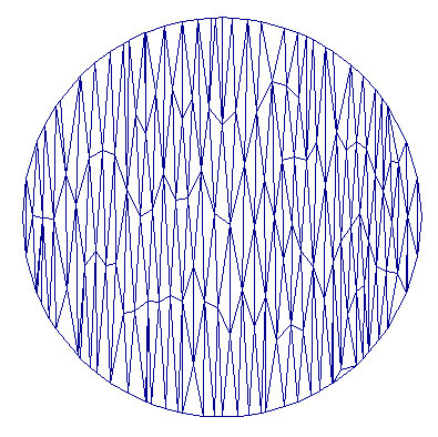
Figure 4.2: Comparison of an isotropic and an anisotropic mesh. The figure on the left shows the lack of directional bias expected for a mesh suitable for the isotropic problem, while the figure on the right is suitable for the case where the conductivity is greater in the $y$-direction then in the $x$-direction.

Figure 4.3: Interpolation quality of adapted meshes measured by the $L_{2}$-norm error in a linear interpolation of $s(x,y)$. Error diminishes as ${\cal O}(N^{-1})$ in both cases, but is offset by a factor of about 4 in the adapted anisotropic meshes.

Figure 4.4: Interpolation quality of adapted meshes measured by the $h^{1}$-semi-norm error in a linear interpolation of $s(x,y)$. Error diminishes as ${\cal O}(N^{-\frac{1}{2}})$ in both cases, but is offset by a factor of about 3 in the adapted anisotropic meshes.

Figure 4.5: Matrix conditioning quality of adapted meshes measured by the spectral condition number $\kappa_{2}$ of the stiffness matrix. The condition number grows as ${\cal O}(N)$ in both cases, but is offset by a factor of about 5 in the adapted anisotropic meshes.

5 Relation with inverse homogenization

Consider the following sequence of PDEs indexed by $\epsilon$.

$$\left\{\begin{aligned} -\operatorname{div}\left(\sigma(\frac{x}{\epsilon})\nabla u_{\epsilon}\right)&=f,\enspace&x\in\Omega,\\ u&=0,\enspace&x\in\partial\Omega.\end{aligned}\right.$$ (5.1)

Assuming that $y\rightarrow\sigma(y)$ is periodic (with in $L^{\infty}(\mathbb{T}^{d})$, where $\mathbb{T}^{d}$ is the $d$-dimensional unit torus) we know from classical homogenization theory [18] that $u_{\epsilon}$ converges towards $u_{0}$ as $\epsilon\downarrow 0$ where $u_{0}$ is the solution of the following PDE

$$\left\{\begin{aligned} -\operatorname{div}\left(\sigma_{e}\nabla u_{0}\right)&=f,\enspace&x\in\Omega,\\ u&=0,\enspace&x\in\partial\Omega.\end{aligned}\right.$$ (5.2)

Moreover $\sigma_{e}$ is constant positive definite $d\times d$ matrix defined by

$$\sigma_{e}:=\int_{\mathbb{T}^{d}}\sigma(y)(I_{d}+\nabla\chi(y))$$ (5.3)

where the entries of the vector field $\chi:=(\chi_{1},\ldots,\chi_{d})$ are solutions of the cell problems

$$\left\{\begin{aligned} -\operatorname{div}\left(\sigma(y)\nabla(y_{i}+\chi_{i}(y))\right)=0,\enspace&y\in\mathbb{T}^{d},\\ \chi_{i}\in H^{1}(\mathbb{T}^{d})\quad\int_{\mathbb{T}^{d}}\chi_{i}(y)=0\end{aligned}\right.$$ (5.4)

Consider the following problem:

Inverse homogenization problem:

Given the effective matrix $\sigma_{e}$ find $\sigma$.

This problem belongs to a class of problems in engineering called inverse homogenization, structural or shape optimization corresponding to the computation of the microstructure of a material from its effective or homogenized properties or the optimization of effective properties with respect to microstructures belonging to an “admissible set”. These problems are known to be ill posed in the sense that they don’t admit a solution but a minimizing sequence of designs. It is possible to characterize the limits of the sequences by following the theory of G-convergence [75] as observed in [57, 62]. For non-symmetric matrices the notion of H-convergence has been introduced [61, 62]. The modern theory for the optimal design of materials is the relaxation method through homogenization [62, 57, 29, 58, 79]. This theory has lead to numerical methods allowing for the design of nearly optimal micro-structures [17, 8, 56]. We also refer to [60, 81, 30] for the related theory of composite materials.

In this paper we observe that at least for the conductivity problem in dimension it is possible to transform the problem of looking for an optimal solution within a highly non-linear into the problem of looking for an optimal solution within a linear space, as illustrated by theorem 5.1 and Figure 5.1 for which efficient optimization algorithms could be developed.

Figure 5.1: Illustration of theorem 5.1.

Define $F(y):=y+\chi(y)$ where $\chi$ is defined by (5.4).

5.1 Theorem.

Let $Q$ be defined by (2.24), then

1. $Q$ is divergence-free, periodic and associated with a convex function $s$ on $[0,1]^{2}$ through (2.42).

2. $$\sigma_{e}=\int_{\mathbb{T}^{d}}Q(y)\,dy$$ (5.5)

3. If $\sigma$ is isotropic then

   $$\sigma=\sqrt{\det(Q)\circ G^{-1}}I_{d}$$ (5.6)

   where $G(y):=y+\bar{\chi}$, $\bar{\chi}:=(\bar{\chi}_{1},\bar{\chi}_{2})$ and

   $$\left\{\begin{aligned} -\operatorname{div}\left(\frac{Q}{\sqrt{\det(Q)}}(y)\nabla(y_{i}+\bar{\chi}_{i}(y))\right)=0,\enspace&y\in\mathbb{T}^{d},\\ \bar{\chi}_{i}\in H^{1}(\mathbb{T}^{d})\quad\int_{\mathbb{T}^{d}}\bar{\chi}_{i}(y)=0\end{aligned}\right.$$ (5.7)

The problem of the computation of the microstructure of a material from macroscopic information is not limited to inverse homogenization. Indeed in many ill posed inverse problems one can choose a scale coarse enough at which the problem admits a unique solution. Hence these problems can be formulated as the composition of a well posed (eventually non-linear) problem with an inverse homogenization problem. The approach proposed here can also used to transform these problems (looking for an optimal solution within a highly non-linear, non-convex space) into the problem of looking for an optimal solution within a linear space, as illustrated in Figure 5.2 for which efficient optimization algorithms can be used. As an example, we examine Electric Impedance Tomography (EIT) in subsection 6.1.

Figure 5.2: Relationships between spaces in inverse homogenization.

6 Electric Impedance Tomography

We now apply our new approach to the inverse problem referred to as Electric Impedance Tomography (EIT), which considers the electrical interpretation of (2.1). The goal is to determine electrical conductivity from boundary voltage and current measurements, whereupon $\sigma(x)$ is an image of the materials comprising the domain. Boundary data is given as the Dirichlet-to-Neumann (DtN) map, $\Lambda_{\sigma}:H^{\frac{1}{2}}(\partial\Omega)\rightarrow H^{-\frac{1}{2}}(\partial\Omega)$, where this operator returns the electrical current pattern at the boundary for a given boundary potential.

$\Lambda_{\sigma}$ can be sampled by solving the Dirichlet problem

$$\left\{\begin{aligned} -\operatorname{div}(\sigma\nabla u)&=0,\enspace&x\in\Omega,\\ u&=g,\enspace&x\in\partial\Omega,\end{aligned}\right.$$ (6.1)

and measuring the resulting Neumann data $f=\sigma\frac{\partial u}{\partial n},x\in\partial\Omega$. (In EIT, Neumann data is interpreted as electric current.) Although boundary value problem (6.1) is not identical to the basic problem (2.1), we can still appeal to the homogenization results in [68] provided we restrict $g\in W^{2-\frac{1}{p},p}$, in which case, we again have regular homogenization solutions $\hat{u}\in W^{2,p}$, that is, those obtained by applying conductivity $Q(x)$ or $s(x)$. If $p>2$, a Sobolev embedding theorem gives $\hat{u}\in C^{1,\alpha},\alpha>0$, already seen in Section 2.1, although this restriction is not necessary for this section.

The EIT problem was first identified in the mathematics literature in the seminal 1980 paper by Calderón [28], although the technique had been known in geophysics since the 1930s. We refer to [20] and references therein for simulated and experimental implementations of the method proposed by Calderón. From the work of Uhlmann, Sylvester, Kohn, Vogelius, Isakov and more recently, Alessandrini and Vessella, we know that complete knowledge of $\Lambda_{\sigma}$ uniquely determines an isotropic $\sigma(x)\in L^{\infty}(\Omega)$, where $\Omega\subset\mathbb{R}^{d},d\geq 2$  [7, 52, 78, 47].

For a given diffeomorphism $F$ from $\Omega$ onto $\Omega$, write

$$F_{\ast}\sigma:=\frac{(\nabla F)^{T}\sigma\nabla F}{\det(\nabla F)}\circ F^{-1}$$ (6.2)

It is known [43] (see also [42, 77, 64, 14]) that for any diffeomorphism $F:\Omega\rightarrow\Omega,\quad F\in H^{1}(\Omega)$, the transformed conductivity $\tilde{\sigma}(x)=F_{\ast}\sigma(x)$ has the same DtN map as the original conductivity. If $\sigma(x)$ is not isotropic, then $\tilde{\sigma}\neq\sigma$. However, as shown in [14], this is the only manner in which $\sigma(x)\in L^{\infty}(\Omega)$ can be non-unique.

Let $\Sigma(\Omega)$ be set of uniformly elliptic and bounded conductivities on $\Omega\in\mathbb{R}^{2}$, that is,

$$\Sigma(\Omega)=\{\sigma\in L^{\infty}(\Omega;\mathbb{R}^{2\times 2})\,\mid\,\sigma=\sigma^{T},0<\lambda_{\min}(\sigma)<\lambda_{\max}(\sigma)<\infty\}.$$ (6.3)

The main result of [14] is that $\Lambda_{\sigma}$ uniquely determines the equivalence class of conductivities

$$E_{\sigma}= \{\sigma_{1}\in\Sigma(\Omega)\mid\sigma_{1}=F_{\ast}\sigma,$$ (6.4)

$$F:\Omega\rightarrow\Omega\quad\text{is an $H^{1}$-diffeomorphism and $F\mid_{\partial\Omega}=x$}\}.$$

It has also been shown that there exists at most $\gamma\in E_{\sigma}$ such that $\gamma$ is isotropic [14].

Our contributions in this section are as follows:

• Proposition 6.1 gives an alternate and very simple proof of the uniqueness of an isotropic $\sigma\in E_{\sigma}$. This is in contrast to Lemma 3.1 of [14], which appeals to quasi-conformal mappings. Moreover, Proposition (6.1) identifies isotropic $\gamma$ by explicit construction from an abribitrary $M\in E_{\sigma}$.

• Proposition 6.2 shows that there exists equivalent classes $E_{\sigma}$ admitting no isotropic conductivities.

Proposition 6.3 shows that a given $\sigma\in\Sigma(\Omega)$ there exists a unique divergence-free matrix $Q$ such that $\Lambda_{Q}=\Lambda_{\sigma}$. It has been brought to our attention that proposition 6.3 has also been proven in [5]. Hence, although for a given DtN map there may not exist an isotropic $\sigma$ such that $\Lambda=\Lambda_{\sigma}$, there always exists a unique divergence-free $Q$ such that $\Lambda=\Lambda_{Q}$. This is of practical importance since the medium to be recovered in a real application may not be isotropic and the associated EIT problem may not admit an isotropic solution. Although the inverse of the map $\sigma\rightarrow\Lambda_{\sigma}$ is not continuous with respect to the topology of $G$-convergence when $\sigma$ is restricted to the set of isotropic matrices, it has also been shown in section 3 of [5] that this inverse is continuous with respect to the topology of $G$-convergence when $\sigma$ is restricted to the set of divergence-free matrices.

We suggest from the previous observations and from theorem 2.20 that the space of convex functions on $\Omega$ is a natural space in which to look for a parametrization of solutions of the EIT problem. In particular if an isotropic solution does exist, proposition (6.1) allows for its recovery through the resolution the PDE (6.6) involving the hessian of that convex function.

6.1 Proposition.

Let $\gamma\in E_{\sigma}$ such that $\gamma$ is isotropic. Then in dimension $d=2$,

1. $\gamma$ is unique.

2. For any $M\in E_{\sigma}$

   $$\gamma=\sqrt{\det(M)\circ G^{-1}}\,I_{d},$$ (6.5)

   where $G=(G_{1},G_{2})$ are the harmonic coordinates associated to $\frac{M}{\sqrt{\det(M)}}$, that is, $G$ is the solution of

   $$\left\{\begin{aligned} \operatorname{div}\Big{(}\frac{M}{\sqrt{\det(M)}}\nabla G_{i}\Big{)}&=0,\enspace&x\in\Omega,\\ G_{i}(x)&=x_{i},\enspace&x\in\partial\Omega.\end{aligned}\right.$$ (6.6)

3. $G=F^{-1}$ where $G$ is the transformation given by (6.6), and $F$ is the diffeomorphism mapping $\gamma$ onto $M$ through equation (6.2).

Proof.

The proof is identical to the proof of Theorem 2.15. ∎

6.2 Proposition.

If $\sigma$ is a non isotropic, symmetric, definite positive, constant $2\times 2$ matrix, then there exists no isotropic $\gamma\in E_{\sigma}$.

Proof.

Let us prove the proposition by contradiction. Assume that $\gamma$ exists. Then, it follows from Proposition 6.1 that $\gamma$ is constant and equal to $\sqrt{\det(\sigma)}I_{d}$. Moreover, it follows from (6.6) that $F^{-1}(x)=x$. Using

$$\sigma=\frac{(\nabla F)^{T}\gamma\nabla F}{\det(\nabla F)}\circ F^{-1}$$ (6.7)

we obtain that $\sigma$ is isotropic which is a contradiction. ∎

6.3 Proposition.

Let $\sigma\in E_{\sigma}$. Then in dimension $d=2$,

1. There exists a unique $Q$ such that $Q$ is a positive, symmetric divergence-free and $Q=F_{\ast}\sigma$. Moreover, $F$ are the harmonic coordinates associated to $\sigma$ given by (2.2).

2. $Q$ is bounded and uniformly elliptic if and only if the non-degeneracy condition (2.4) is satisfied for an arbitrary $M\in E_{\sigma}$.

3. $Q$ is the unique positive, symmetric, and divergence-free matrix such that $\Lambda_{Q}=\Lambda_{\sigma}$.

Proof.

The existence of $Q$ follows from Proposition 2.14. Let us prove the uniqueness of $Q$. If

$$Q=\frac{(\nabla F)^{T}\sigma\nabla F}{\det(\nabla F)}\circ F^{-1}$$ (6.8)

is divergence free, then for all $l\in\mathbb{R}^{d}$ and $\varphi\in C_{0}^{\infty}(\Omega)$

$$\int_{\Omega}(\nabla\varphi)^{T}Q\cdot l=0.$$ (6.9)

Using the change of variables $y=F(x)$ we obtain that

$$\int_{\Omega}(\nabla\varphi)^{T}Q\cdot l=\int_{\Omega}(\nabla(\varphi\circ F))^{T}\sigma\nabla F\cdot l.$$ (6.10)

It follows that $F$ are the harmonic coordinates associated to $\sigma$ which proves the uniqueness of $Q$. The second part of the proposition follows from Proposition 2.14. ∎

6.1 Numerical reconstructions with incomplete boundary measurements using geometric homogenization

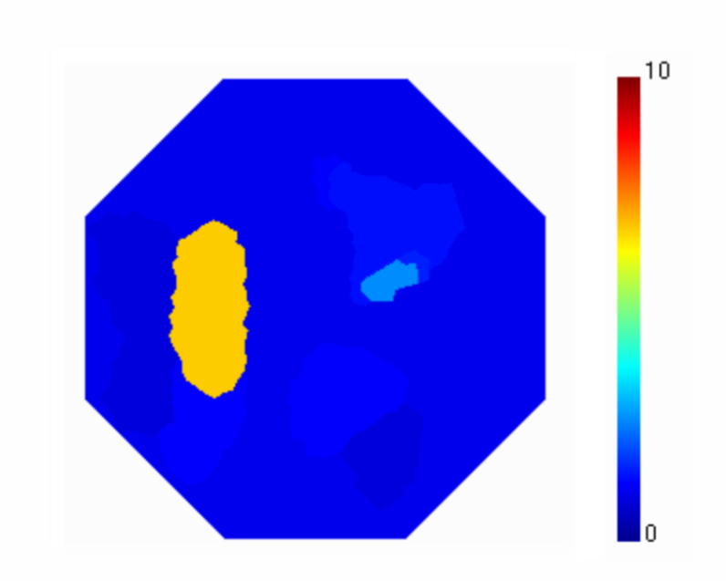
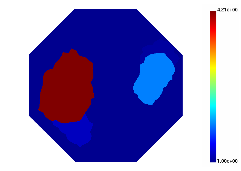
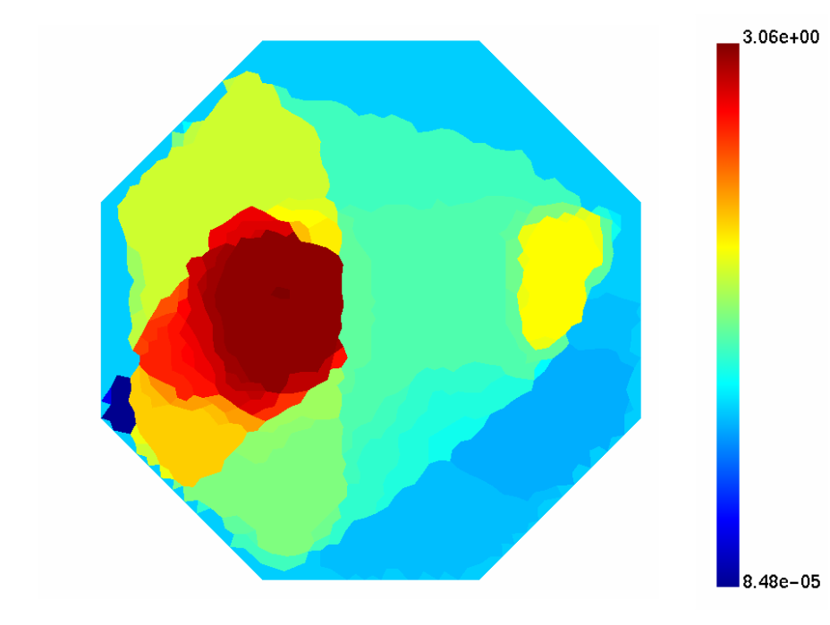
Figure 6.2: Output of the harmonic coordinate iteration. The figure on the top left is the coarse mesh produced by simulated annealing, the input to the harmonic coordinate iteration. Left to right, top to bottom, the remaining three images show the progression of the iteration at 1, 10, and 20 steps, showing its instability. The true conductivity is that of Figure 6.1.

We close by examining two numerical methods for recovering conductivities from incomplete boundary data using the ideas of geometric homogenization. By incomplete we mean that potentials and currents are measured at only a finite number of points of the boundary of the domain. (For example, we have data at $8$ points in Figure 6.2 for the medium shown in Figure 6.1.)

The first method is an iteration between the harmonic coordinates $F(x)$ and the conductivity $\sigma(x)$. The second recovers $s^{h}(x)$ from incomplete boundary data, and from $s^{h}(x)$ we compute $q^{h}(x)$, then $Q$. Both methods regularize the reconstruction in a natural way as to provide super-resolution of the conductivity in a sense we now make precise.

The inverse conductivity problem with an imperfectly known boundary has also been considered in [54]. We refer to [50] and reference therein for an analysis of the reconstruction of realistic conductivities from noisy EIT data (using the D-bar method by studying its application to piecewise smooth conductivities).

Even with complete boundary data this inverse problem is ill-posed with respect to the resolution of $\sigma(x)$. The Lipschitz stability estimate in [7] states

$$\lVert\sigma^{(1,N)}(x)-\sigma^{(2,N)}(x)\rVert_{L^{\infty}}\\ \leq C(N)\lVert\Lambda_{\sigma^{(1,N)}}-\Lambda_{\sigma^{(2,N)}}\rVert_{{\cal L}(H^{\frac{1}{2}}(\partial\Omega),H^{-\frac{1}{2}}(\partial\Omega))},$$ (6.11)

where ${\cal L}(H^{\frac{1}{2}}(\partial\Omega),H^{-\frac{1}{2}}(\partial\Omega))$ is the natural operator norm for the DtN map. $\sigma^{(j,N)}(x)$ are scalar conductivities satisfying the ellipticity condition $0<\lambda\leq\sigma(x)\leq\lambda^{-1}$ almost everywhere in $\Omega$ and belonging to a finite-dimensional space such that

$$\sigma^{(j,N)}(x)=\sum_{i=1}^{N}\sigma^{(j,N)}_{i}z_{i}^{(N)}(x)$$ (6.12)

for known basis functions $z_{i}^{(N)}(x)$. Thus, the inverse problem in this setting is to determine the real numbers $\sigma^{(j,N)}_{i}$ from the given DtN map $\Lambda_{\sigma^{(j,N)}}$.

The Lipschitz constant $C(N)$ depends on $\lambda,\Omega$ and $z_{i}^{(N)}$. As shown by construction in [71], when $z_{i}^{(N)}$ are characteristic functions of $N$ disjoint sets covering $\Omega\subset\mathbb{R}^{d}$, the bound

$$C(N)\geq A\exp\left(BN^{\frac{1}{2d-1}}\right)$$ (6.13)

for absolute constants $A,B>0$ is sharp. That is, the amplification of error in the recovered conductivity with respect to boundary data error increases exponentially with $N$.

From (6.13), we infer a resolution limit on the identification of $\sigma(x)$. Setting $\bar{C}$ our upper tolerance for the amplification of error in recovering $\sigma(x)$ with respect to boundary data error, and introducing resolution $\bar{r}=N^{-1/d}$, which scales with length, we have

$$\bar{r}\geq\left(\frac{1}{B}\log\frac{\bar{C}}{A}\right)^{-\frac{2d-1}{d}}.$$ (6.14)

We refer to any features of $\sigma(x)$ resolved at scales greater than this limit as stably-resolved and knowledge of features below this limit as super-resolved.

6.1.1 Harmonic coordinate iteration.

The first method provides super-resolution in two steps. First, we stably-resolve conductivity using a resistor-network interpretation. From this stable resolution, we super-resolve conductivity by computing a function $\sigma(x)$ and its harmonic coordinates $F(x)$ consistent with the stable resolution.

To solve for the conductivity at a stable resolution, we consider a coarse triangulation of $\Omega$. Assigning a piecewise linear basis over the triangulation gives the edge-wise conductivies

$$q_{ij}^{h}:=-\int_{\Omega}(\nabla\varphi_{i})^{T}Q(x)\nabla\varphi_{j}\,dx.$$ (2.15)

As we have already examined, when $\sigma(x)$ (hence $Q(x)$) is known, so too are the $q_{ij}^{h}$. The discretized inverse problem is, given data at boundary vertices, determine an appropriate triangulation of the domain and the $q_{ij}^{h}$ over the edges of the triangulation. We next specify our discrete model of conductivity in order to define what we mean by “boundary data.”

Let ${\cal V}_{I}$ be the set of interior vertices of a triangulation of $\Omega$, and let ${\cal V}_{B}$ be the boundary vertices, namely, the set of vertices on $\partial\Omega$. Let the cardinality of ${\cal V}_{B}$ be $V_{B}$. Suppose vector $u^{(k)}$ solves the matrix equation

$$\left\{\begin{aligned} \sum_{j\sim i}q^{h}_{ij}(u^{(k)}_{i}-u^{(k)}_{j})&=0,\enspace&i\in{\cal V}_{I},\\ u^{(k)}_{i}&=g^{(k)}_{i},\enspace&i\in{\cal V}_{B},\end{aligned}\right.$$ (6.15)

where $g^{(k)}$ is given discrete Dirichlet data. Then we define

$$f^{(k)}_{i}=\sum_{j\sim i}q^{h}_{ij}(u^{(k)}_{i}-u^{(k)}_{j}),\enspace i\in{\cal V}_{B}$$ (6.16)

as the discrete Neumann data. The $V_{B}$ linearly independent $g^{(k)}$ and their associated $f^{(k)}$ together determine the matrix $\Lambda^{{\cal V}_{B}}_{q^{h}}$, which we call the discrete Dirichlet-to-Neumann map. $\Lambda^{{\cal V}_{B}}_{q^{h}}$ is linear, symmetric, and has the vector $g=(1,1,\ldots,1)$ as its nullspace. Hence, $\Lambda^{{\cal V}_{B}}_{q^{h}}$ has $V_{B}(V_{B}-1)/2$ degrees of freedom.

In practise, the discrete DtN map is provided as problem data without a triangulation specified: only the boundary points where the Dirichlet and Neumann data are experimentally collected are given. We refer to this experimentally-determined discrete DtN map as $\Lambda^{{\cal V}_{B}}_{\sigma}$.

We are also aware that to make sense in the homogenization setting, the $q^{h}_{ij}$ must be discretely divergence-free. That is, we require that

$$\sum_{j\sim i}q^{h}_{ij}(x^{(p)}_{i}-x^{(p)}_{j})=0,\enspace i\in{\cal V}_{I},\enspace p=1,2,$$ (6.17)

where $(x^{(1)}_{i},x^{(2)}_{i})$ is the $xy$-location of vertex $i$.

Set ${\cal T}^{{\cal V}_{B}}$ the set of triangulations having boundary vertices ${\cal V}_{B}$ specified by $\Lambda^{{\cal V}_{B}}_{\sigma}$, and $\{q^{h}_{ij}\}$ the edge-values over ${\cal T}^{{\cal V}_{B}}$. The complete problem is

$$\left\{\begin{aligned} &\mathop{\text{minimise}}_{{\cal T}^{{\cal V}_{B}},\{q^{h}_{ij}\}}\enspace\lVert\Lambda^{{\cal V}_{B}}_{q^{h}}-\Lambda^{{\cal V}_{B}}_{\sigma}\rVert_{\ast},\\ &\text{subject to}\enspace\{q^{h}_{ij}\}\,\text{discretely divergence-free}.\end{aligned}\right.$$ (6.18)

The norm $\lVert\cdot\rVert_{\ast}$ is a suitable matrix norm—as a form of regularization, we use a thresholded spectral norm which under-weights error in the modes associated to the smallest eigenvalues. We solve this non-convex constrained problem using Constrained Simulated Annealing (CSA). See [82], for example, for details on the CSA method.

EIT has already been cast in a similar form in [22], where edge-based data was solved for using a finite-volume treatment, interpreting edges of the graph which connects adjacent cells as electrical conductances. They determine the edge values using a direct calculation provided by the inverse theory for resistor networks [31, 32]. Although our work shares some similarities with this prior art, we do not assume that a connectivity is known a priori.

An inversion algorithm for tomographic imaging of high contrast media based on a resistor network theory has also been introduced in [21]. The algorithm of [21] is based on the results of an asymptotic analysis of the forward problem showing that when the contrast of the conductivity is high, the current flow can be roughly approximated by that of a resistor network. Here our algorithm is based on geometric structures hidden in homogenization of divergence form elliptic equations with rough coefficients.

Given an optimal triangulation ${\cal T}^{\ast}$ and its associated stably-resolved $\{q^{h}_{ij}\}$ representing conductivity, we now compute a fine-scale conductivity $\sigma^{f}(x)$ consistent with our edge values, as well as its harmonic coordinates $F(x)$. To help us super-resolve the conductivity, we also regularize $\sigma^{f}(x)$.

Set ${\cal T}^{f}$ a triangulation which is a refinement of triangulation ${\cal T}^{\ast}$ from the solution to the stably-resolved problem. Let $\sigma^{f}(x)$ be constant on triangles of $T^{f}$. Suppose coordinates $F(x)$ are given, and solve

$$\left\{\begin{aligned} &\mathop{\text{minimise}}\enspace\lVert\sigma^{f}(x)\rVert_{\ast},\\ &\text{subject to}\enspace-\int_{\Omega}(\nabla(\varphi_{i}\circ F))^{T}\sigma^{f}(x)\nabla(\varphi_{j}\circ F)=q^{h}_{ij},\enspace i,j\in{\cal T}^{\ast}.\end{aligned}\right.$$ (6.19)

Here, $\lVert\cdot\rVert_{\ast}$ is some smoothness measure of $\sigma^{f}(x)$. Following the success of regularization by total variation norms in other contexts, see [51, 4] for example (in particular we refer to [72] and references therein for convergence results the regularization of the inverse conductivity problem with discontinuous conductivities using total variation and the Mumford-Shah functional.), we choose

$$\lVert z(x)\rVert_{\ast}=\lVert z(x)\rVert_{\text{TV}}:=\int_{\Omega}\lvert\nabla z(x)\rvert.$$ (6.20)

This norm makes particular sense for typical test cases, where the conductivity takes on a small number of constant values. This “cartoon-like” scenario is common where a small blob of unusual material is included within a constant background material. The constraints in (6.19) are linear in the values of $\sigma^{f}(x)$ on triangles of ${\cal T}^{f}$, and the norm is convex, so (6.19) is a convex optimization problem. In particular, it is possible to recast (6.19) as a linear program, see [24], for example. We then use the GNU Linear Programing Kit to do the optimization of this resulting linear program [3]. Note that we build our refined triangulation using Shewchuk’s Triangle program [73].

The harmonic coordinates $F(x)$ are not in general known. We set $F(x)=x$ initially, and following the solution of (6.19), we compute

$$\left\{\begin{aligned} -\operatorname{div}(\sigma^{f}\nabla F)&=0,\enspace&x\in\Omega,\\ F&=x,\enspace&x\in\partial\Omega,\end{aligned}\right.$$ (6.21)

using $\sigma^{f}(x)$ from the previous step. We can now iterate, returning to solve (6.19) with these new harmonic coordinates.

Figures 6.1 and 6.2 show the results of a numerical experiment illustrating the method. In particular, the harmonic coordinate iteration resolves details of the true conductivity at scales below that of the coarse mesh used to resolve $\{q^{h}_{ij}\}$. We observe numerically that this iteration can become unstable and fail to converge. However, before becoming unstable the algorithm indeed super-resolves the conductivity. We believe that this algorithm can be stabilized and plan to investigate its regularization in a future paper.

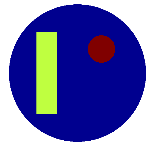
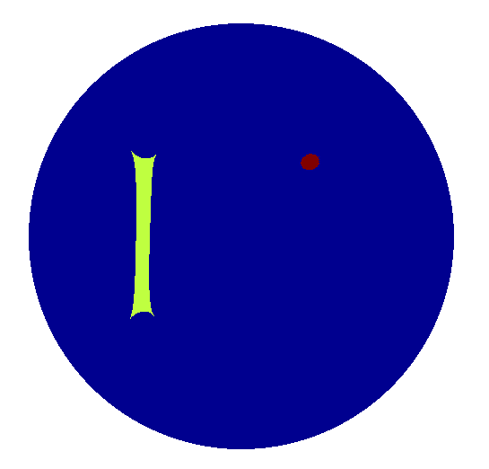
Figure 6.1: A sample isotropic conductivity for testing reconstruction. The image on the left is $\sigma$, while the image on the right is $\sqrt{\det Q}=\sigma\circ F^{-1}$. The dark blue background has conductivity 1.0, the red circle has conductivity 10.0 and the yellow bar has conductivity 5.0. In this case, all of the features shrink in harmonic coordinates.

6.1.2 Divergence-free parameterization recovery.

Our second numerical method computes $s(x)$ from boundary data in one step. In essence, we recover the divergence-free conductivity consistent with the boundary data, without concern for the fine-scale conductivity that gives rise to the coarse-scale anisotropy.

We begin by tessellating $\Omega$ by a fine-scale Delaunay triangulation, and we parameterize conductivity by $s^{h}_{i}$, the piecewise linear interpolants of $s(x)$ over vertices of the triangulation. From the $s^{h}_{i}$, we can compute $q^{h}_{ij}$ using the hinge formula in order to solve the discretized problem (6.15). This determines the discrete DtN map $\Lambda_{s^{h}}$ in this setting.

We shall also need a relationship between the $s^{h}_{i}$ and $Q^{h}_{ijk}$, an approximation of $Q(x)$ constant on triangles. One choice is to presume that $s(x)$ can be locally interpolated by a quadratic polynomial at the vertices of each triangle, and the opposite vertices of its three neighbours, see Figure 6.3. Taking second partial derivatives of this quadratic interpolant gives a linear relationship between $Q^{h}_{ijk}$ and the six nearest $s^{h}_{i}$. This quadratic interpolation presents a small difficulty, as triangles at the edge of $\Omega$ have at most two neighbours. Our solution is to place ghost vertices outside the domain near each boundary edge, thus extending the domain of $s(x)$ and adding points where $s^{h}_{i}$ must be determined.

Figure 6.3: Stencil for approximating $Q(x)$ on triangle $ijk$ from the interpolants $s^{h}_{i}$ at nearby vertices.

We solve for the $s^{h}_{i}$ using optimization by an interior point method. Although the algorithm we choose is intended for convex optimization—the non-linear relationship between $\Lambda_{s^{h}}$ and the $s^{h}_{i}$ makes the resulting problem non-convex—we follow the practise in the EIT literature of relying on regularization to make the algorithm stable [23, 34]. We thus solve

$$\left\{\begin{aligned} &\text{minimise}\enspace\frac{1}{2}\sum_{k=1}^{K}\lVert\Lambda_{s^{h}}g^{(k)}-f^{(k)}\rVert^{2}_{L^{2}(\partial\Omega)}+\alpha\lVert\text{tr}\,Q^{h}\rVert_{\text{TV}},\\ &\text{subject to}\enspace q^{h}_{ij}\geq 0.\end{aligned}\right.$$ (6.22)

We use IpOpt software package for the optimization [1].

The data are provided as $K$ measured Dirichlet-Neumann pairs of data, $\{(g^{(k)},f^{(k)})\}$, and the Tikhonov parameter $\alpha$ is determined experimentally (a common method is the L-curve method). Again, the total variation norm is used to evaluate the smoothness of the conductivity. We could just as well regularize using $\det Q$ rather than $\text{tr}\,Q$. Using the trace makes the problem more computationally tractable (the Jacobian is easier to compute), and our experience with such optimizations shows that regularizing with respect to the determinant does not improve our results. We compute the Jacobian of the objective’s “quadratic” term using a primal-adjoint method, see [34], for example.

We constrain $q^{h}_{ij}\geq 0$ on all edges, despite the possibility that our choice of triangulation may require that some edges should have negative values. Our reasons for this choice are practical: edge-flipping in this case de-stabilizes the interior point method. Moreover, numerical experiments using triangulations well-adapted to $\sigma(x)$ do not give qualitatively better results.

Figures 6.4 and 6.5 show reconstructions of the conductivities in Figures 6.1 and 2.2, respectively. We include the reconstruction of the conductivity in Figure 6.1 only to show that our parameterization can resolve this test case, a typical one in the EIT literature. For such tests recovering “cartoon blobs,” our method does not compete with existing methods such as variational approaches [23], or those based on quasi-conformal mappings [46, 49]. Our recovery of the conductivity in Figure 2.2, however, achieves a reconstruction, to our knowledge, which has not previously been realized. The pitch of the laminations in this test case are below a reasonable limit of stable resolution. Hencee do not aim to recover the laminations themselves, but we do recover their up-scaled representation. The anisotropy of this up-scaled representation is apparent in Figure 6.5. Admitting the possibility of recovering anisotropic, though divergence-free, conductivities by parameterizing conductivity by $s(x)$ gives a sensical recovered conductivity. Owing to the stable resolution limit, parameterizing $\sigma(x)$ directly, by a usual parameterization—such as the linear combination in (6.12), choosing $z_{i}(x)$ as characteristic functions—is not successful.

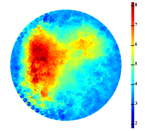
Figure 6.4: Reconstruction of the isotropic conductivity in Figure 6.1. The left-hand figure shows $\text{tr}\,Q$, while the right-hand figure shows $\sqrt{\det Q}$. The reconstruction blurs the original $\sigma$, similar to other methods in the literature, but does not underestimate the dynamic range of the large rectangle.

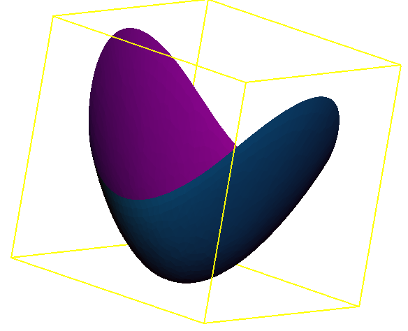
Figure 6.5: Anisotropic reconstruction showing the parameterisation $s(x)$ we recover using EIT (left image), and the pattern of anisotropy we see by rendering the orientation of the maximal eigenvalue of $Q$ (right image). The colour-bar in the right image indicates the strength of the anisotropy as $\lvert\lambda_{\max}-\lambda_{\min}\rvert/\text{tr}\,Q$.

References

- [1] IpOpt, Interior Point Optimizer, version 3.2.4, https://projects.coin-or.org/Ipopt.
- [2] Cgal, Computational Geometry Algorithms Library, version 3.3.1, http://www.cgal.org.
- [3] GNU Linear Programming Kit, http://www.gnu.org/software/glpk/.
- [4] R. Acar and C. R. Vogel, Analysis of bounded variation penalty methods for ill-posed problems, Inverse Problems 10 (1994), 1217–1229.
- [5] Giovanni Alessandrini and Elio Cabib, Determining the anisotropic traction state in a membrane by boundary measurements, Inverse Probl. Imaging 1 (2007), no. 3, 437–442. MR MR2308972 (2008h:35045)
- [6] Giovanni Alessandrini and Vincenzo Nesi, Univalent -harmonic mappings: connections with quasiconformal mappings, J. Anal. Math. 90 (2003), 197–215. MR MR2001070 (2004g:30032)
- [7] Giovanni Alessandrini and Sergio Vessella, Lipschitz stability for the inverse conductivity problem, Advances in Applied Mathematics 35 (2005), 207–241.
- [8] Grégoire Allaire, Shape optimization by the homogenization method, Applied Mathematical Sciences, vol. 146, Springer-Verlag, New York, 2002. MR MR1859696 (2002h:49001)
- [9] Pierre Alliez, David Cohen-Steiner, Mariette Yvinec, and Mathieu Desbrun, Variational tetrahedral meshing, ACM Transactions on Graphics (SIGGRAPH ’05) 24 (2005), no. 3, 617–625, http://www.geometry.caltech.edu/pubs/ACYD05.pdf.
- [10] Alano Ancona, Private communication between A. Ancona and H. Owhadi reported in subsection 6.6.2 of http://www.acm.caltech.edu/õwhadi/publications/phddownload.htm (1999).
- [11] Alano Ancona, Some results and examples about the behavior of harmonic functions and Green’s functions with respect to second order elliptic operators, Nagoya Math. J. 165 (2002), 123–158. MR MR1892102 (2002m:31012)
- [12] Todd Arbogast and Kirsten J. Boyd, Subgrid upscaling and mixed multiscale finite elements, SIAM J. Numer. Anal. 44 (2006), no. 3, 1150–1171 (electronic). MR MR2231859 (2007k:65165)
- [13] Todd Arbogast, Chieh-Sen Huang, and Song-Ming Yang, Improved accuracy for alternating-direction methods for parabolic equations based on regular and mixed finite elements, Math. Models Methods Appl. Sci. 17 (2007), no. 8, 1279–1305. MR MR2342991
- [14] Kari Astala, Matti Lassas, and Lassi Paivarinta, Calderon’s inverse problem for anisotropic conductivity in the plane, Communications in Partial Differential Equations 30 (2005), no. 2, 207–224, DOI http://arxiv.org/abs/math/0401410v1.
- [15] I. Babuška and J. E. Osborn, Generalized finite element methods: their performance and their relation to mixed methods, SIAM J. Numer. Anal. 20 (1983), no. 3, 510–536. MR MR701094 (84h:65076)
- [16] Ivo Babuška, Gabriel Caloz, and John E. Osborn, Special finite element methods for a class of second order elliptic problems with rough coefficients, SIAM J. Numer. Anal. 31 (1994), no. 4, 945–981. MR MR1286212 (95g:65146)
- [17] M. P. Bendsøe and O. Sigmund, Topology optimization, Springer-Verlag, Berlin, 2003, Theory, methods and applications. MR MR2008524 (2005e:74046)
- [18] A. Bensoussan, J. L. Lions, and G. Papanicolaou, Asymptotic analysis for periodic structure, North Holland, Amsterdam, 1978.
- [19] Leonid Berlyand and Houman Owhadi, A new approach to homogenization with arbitrarily rough coefficients for scalar and vectorial problems with localized and global pre-computing., to appear, http://arxiv.org/abs/0901.1463 (2009).
- [20] Jutta Bikowski and Jennifer L. Mueller, 2D EIT reconstructions using Calderón’s method, Inverse Probl. Imaging 2 (2008), no. 1, 43–61. MR MR2375322 (2009c:35469)
- [21] Liliana Borcea, James G. Berryman, and George C. Papanicolaou, High-contrast impedance tomography, Inverse Problems 12 (1996), no. 6, 835–858. MR MR1421651
- [22] Liliana Borcea, Vladimir Druskin, and Fernando Guevara Vasquez, Electrical impedance tomography with resistor networks, Inverse Problems 24 (2008), no. 3, 035013, 31. MR MR2421967 (2009e:78027)
- [23] Liliana Borcea, Genetha Anne Gray, and Yin Zhang, Variationally constrained numerical solution of electrical impedance tomography, Inverse Problems 19 (2003), 1159–1184.
- [24] Stephen Boyd and Lieven Vandenberghe, Convex optimization, Cambridge University Press, New York, 2004.
- [25] Andrea Braides, -convergence for beginners, Oxford Lecture Series in Mathematics and its Applications, vol. 22, Oxford University Press, Oxford, 2002. MR MR1968440 (2004e:49001)
- [26] Marc Briane, Graeme W. Milton, and Vincenzo Nesi, Change of sign of the corrector’s determinant for homogenization in three-dimensional conductivity, Arch. Ration. Mech. Anal. 173 (2004), no. 1, 133–150. MR MR2073507
- [27] Luis A. Caffarelli and Panagiotis E. Souganidis, A rate of convergence for monotone finite difference approximations to fully nonlinear, uniformly elliptic PDEs, Comm. Pure Appl. Math. 61 (2008), no. 1, 1–17. MR MR2361302
- [28] A. P. Calderón, On an inverse boundary value problem, Seminar on Numerical Analysis and its Applications to Continuum Physics (Rio de Janerio), Soc. Brasileira de Mathematica, 1980.
- [29] Andrej Cherkaev, Variational methods for structural optimization, Applied Mathematical Sciences, vol. 140, Springer-Verlag, New York, 2000. MR MR1763123 (2001e:74070)
- [30] Andrej Cherkaev and Robert Kohn (eds.), Topics in the mathematical modelling of composite materials, Progress in Nonlinear Differential Equations and their Applications, 31, Birkhäuser Boston Inc., Boston, MA, 1997. MR MR1493036 (98i:73001)
- [31] Edward B. Curtis and James A. Morrow, Determining the resistors in a network, SIAM Journal on Applied Mathematics 50 (1990), no. 3, 931–941.
- [32] , Inverse problems for electrical networks, World Scientific, 2000.
- [33] Ennio De Giorgi, New problems in -convergence and -convergence, Free boundary problems, Vol. II (Pavia, 1979), Ist. Naz. Alta Mat. Francesco Severi, Rome, 1980, pp. 183–194. MR MR630747 (83e:49023)
- [34] David C. Dobson, Convergence of a reconstruction method for the inverse conductivity problem, SIAM Journal on Applied Mathematics 52 (1992), no. 2, 442–458.
- [35] Roger D. Donaldson, Discrete geometric homogenisation and inverse homogenisation of an elliptic operator, Ph.D. thesis, California Institute of Technology, 2008, DOI http://resolver.caltech.edu/CaltechETD:etd-05212008-164705.
- [36] Weinan E, Bjorn Engquist, Xiantao Li, Weiqing Ren, and Eric Vanden-Eijnden, Heterogeneous multiscale methods: a review, Commun. Comput. Phys. 2 (2007), no. 3, 367–450. MR MR2314852 (2008f:74094)
- [37] Y. Efendiev, V. Ginting, T. Hou, and R. Ewing, Accurate multiscale finite element methods for two-phase flow simulations, J. Comput. Phys. 220 (2006), no. 1, 155–174. MR MR2281625 (2007g:76130)
- [38] Y. Efendiev and T. Hou, Multiscale finite element methods for porous media flows and their applications, Appl. Numer. Math. 57 (2007), no. 5-7, 577–596. MR MR2322432 (2008b:76114)
- [39] B. Engquist and P. E. Souganidis, Asymptotic and numerical homogenization, Acta Numerica 17 (2008), 147–190.
- [40] E. De Giorgi, Sulla convergenza di alcune successioni di integrali del tipo dell’aera, Rendi Conti di Mat. 8 (1975), 277–294.
- [41] David Glickenstein, A monotonicity property for weighted Delaunay triangulations, Discrete and Computational Geometry 38 (2007), no. 4, 651–664, http://math.arizona.edu/ glickenstein/monotonic.pdf.
- [42] Allan Greenleaf, Matti Lassas, and Gunther Uhlmann, Anisotropic conductivities that cannot be detected by EIT, Physiological Measurement 24 (2003), 412–420.
- [43] , On nonuniqueness for Calderón’s inverse problem, Mathematical Research Letters 10 (2003), no. 5, 685, DOI http://arxiv.org/abs/math/0302258v2.
- [44] Helmut Harbrecht, Reinhold Schneider, and Christoph Schwab, Sparse second moment analysis for elliptic problems in stochastic domains, Numer. Math. 109 (2008), no. 3, 385–414. MR MR2399150
- [45] Thomas Y. Hou and Xiao-Hui Wu, A multiscale finite element method for elliptic problems in composite materials and porous media, J. Comput. Phys. 134 (1997), no. 1, 169–189. MR MR1455261 (98e:73132)
- [46] D. Isaacson, J. L. Mueller, J. C. Newell, and S. Siltanen, Imaging cardiac activity by the D-bar method for electrical impedance tomography, Physiological Measurement 27 (2006), S43–S50.
- [47] Victor Isakov, Uniqueness and stability in multi-dimensional inverse problems, Inverse Problems 9 (1993), 579–621.
- [48] V. V. Jikov, S. M. Kozlov, and O. A. Oleinik, Homogenization of differential operators and integral functionals, Springer-Verlag, 1991.
- [49] K. Knudsen, J. L. Mueller, and Sl Siltanen, Numerical solution method for the dbar-equation in the plane, Journal of Computational Physics 198 (2004), 500–517.
- [50] Kim Knudsen, Matti Lassas, Jennifer L. Mueller, and Samuli Siltanen, D-bar method for electrical impedance tomography with discontinuous conductivities, SIAM J. Appl. Math. 67 (2007), no. 3, 893–913 (electronic). MR MR2300316 (2007m:35276)
- [51] Roger Koenker and Ivan Mizera, Penalized triograms: Total variation regularization for bivariate smoothing, Journal of the Royal Statistical Society. Series B. Statistical Methodology 66 (2004), no. 1, 145–163.
- [52] R. V. Kohn and M. Vogelius, Determining conductivity by boundary measurements, Communications on Pure and Applied Mathematics 37 (1984), 113–123.
- [53] Robert V. Kohn and Michael Vogelius, Identification of an unknown conductivity by means of measurements at the boundary, Inverse problems (New York, 1983), SIAM-AMS Proc., vol. 14, Amer. Math. Soc., Providence, RI, 1984, pp. 113–123. MR MR773707
- [54] Ville Kolehmainen, Matti Lassas, and Petri Ola, The inverse conductivity problem with an imperfectly known boundary, SIAM J. Appl. Math. 66 (2005), no. 2, 365–383 (electronic). MR MR2203860 (2007f:35298)
- [55] Houman Owhadi Lily Kharevych, Patrick Mullen and Mathieu Desbrun, Homogenization, model coarsening, model reduction, corotational methods., to appear (2009).
- [56] Robert Lipton and Michael Stuebner, Optimization of composite structures subject to local stress constraints, Comput. Methods Appl. Mech. Engrg. 196 (2006), no. 1-3, 66–75. MR MR2270127 (2007m:74106)
- [57] K. A. Lur′e and A. V. Cherkaev, Effective characteristics of composite materials and the optimal design of structural elements, Adv. in Mech. 9 (1986), no. 2, 3–81. MR MR885713 (88e:73019)
- [58] K. A. Lurie, Applied optimal control theory of distributed systems, Mathematical Concepts and Methods in Science and Engineering, vol. 43, Plenum Press, New York, 1993. MR MR1211415 (94d:49001)
- [59] A. Maugeri, D. K. Palagachev, and L. G. Softova, Elliptic and parabolic equations with discontinuous coefficients, Mathematical Research, vol. 109, Wiley-VCH, 2000.
- [60] Graeme W. Milton, The theory of composites, Cambridge Monographs on Applied and Computational Mathematics, vol. 6, Cambridge University Press, Cambridge, 2002. MR MR1899805 (2003d:74077)
- [61] F. Murat and L. Tartar, H-convergence, Séminaire d’Analyse Fonctionnelle et Numérique de l’Université d’Alger (1978).
- [62] F. Murat and L. Tartar, Calcul des variations et homogénéisation, Homogenization methods: theory and applications in physics (Bréau-sans-Nappe, 1983), Collect. Dir. Études Rech. Élec. France, vol. 57, Eyrolles, Paris, 1985, pp. 319–369. MR MR844873 (87i:73059)
- [63] François Murat, Compacité par compensation, Ann. Scuola Norm. Sup. Pisa Cl. Sci. (4) 5 (1978), no. 3, 489–507. MR MR506997 (80h:46043a)
- [64] Adrian I. Nachman, Global uniqueness for a two-dimensional inverse boundary value problem, Annals of Mathematics 142 (1995), 71–96.
- [65] James Nolen, George Papanicolaou, and Olivier Pironneau, A framework for adaptive multiscale methods for elliptic problems, Multiscale Model. Simul. 7 (2008), no. 1, 171–196. MR MR2399542
- [66] Joseph O’Rourke, Computational geometry in c, 2nd ed., Cambridge University Press, New York, 1998.
- [67] H. Owhadi and L. Zhang, Homogenization of the acoustic wave equation with a continuum of scales., Computer Methods in Applied Mechanics and Engineering 198 (2008), no. 2-4, 97–406, Arxiv math.NA/0604380.
- [68] Houman Owhadi and Lei Zhang, Metric-based upscaling, Comm. Pure Appl. Math. 60 (2007), no. 5, 675–723. MR MR2292954
- [69] , Homogenization of parabolic equations with a continuum of space and time scales, SIAM J. Numer. Anal. 46 (2007/08), no. 1, 1–36. MR MR2377253
- [70] Ulrich Pinkall and Konrad Polthier, Computing discrete minimal surfaces and their conjugates, Exp. Math. 2(1) (1993), 15–36.
- [71] Luca Rondi, A remark on a paper by alessandrini and vessella, Advances in Applied Mathematics 36 (2006), 67–69.
- [72] Luca Rondi, On the regularization of the inverse conductivity problem with discontinuous conductivities, Inverse Probl. Imaging 2 (2008), no. 3, 397–409. MR MR2424823
- [73] Jonathan Richard Shewchuk, Triangle: A two-dimensional quality mesh generator and delaunay triangulator, http://www.cs.cmu.edu/~quake/triangle.html.
- [74] S. Spagnolo, Sulla convergenza di soluzioni di equazioni paraboliche ed ellittiche., Ann. Scuola Norm. Sup. Pisa (3) 22 (1968), 571-597; errata, ibid. (3) 22 (1968), 673. MR MR0240443 (39 #1791)
- [75] Sergio Spagnolo, Convergence in energy for elliptic operators, Numerical solution of partial differential equations, III (Proc. Third Sympos. (SYNSPADE), Univ. Maryland, College Park, Md., 1975), Academic Press, New York, 1976, pp. 469–498. MR MR0477444 (57 #16971)
- [76] Theofanis Strouboulis, Lin Zhang, and Ivo Babuška, Assessment of the cost and accuracy of the generalized FEM, Internat. J. Numer. Methods Engrg. 69 (2007), no. 2, 250–283. MR MR2283892 (2008c:65348)
- [77] John Sylvester, An anisotropic inverse boundary value problem, Communications on Pure and Applied Mathematics 43 (1990), 201–232.
- [78] John Sylvester and Gunther Uhlmann, A global uniqueness theorem for an inverse boundary value problem, Annals of Mathematics 125 (1987), 153–169.
- [79] Luc Tartar, An introduction to the homogenization method in optimal design, Optimal shape design (Tróia, 1998), Lecture Notes in Math., vol. 1740, Springer, Berlin, 2000, pp. 47–156. MR MR1804685
- [80] Radu Alexandru Todor and Christoph Schwab, Convergence rates for sparse chaos approximations of elliptic problems with stochastic coefficients, IMA J. Numer. Anal. 27 (2007), no. 2, 232–261. MR MR2317004 (2008b:65016)
- [81] Salvatore Torquato, Random heterogeneous materials, Interdisciplinary Applied Mathematics, vol. 16, Springer-Verlag, New York, 2002, Microstructure and macroscopic properties. MR MR1862782 (2002k:82082)
- [82] Benjamin W Wah and Tao Wang, Simulated annealing with asymptotic convergence for nonlinear constrained global optimization, Proceedings of the 5th International Conference on Principles and Practice of Constraint Programming (London), Lecture Notes In Computer Science, vol. 1713, Springer, 1999, pp. 461–475.