Bayesian analysis of white noise levels in the 5-year WMAP data

Abstract

We develop a new Bayesian method for estimating white noise levels in CMB sky maps, and apply this algorithm to the 5-year WMAP data. We assume that the amplitude of the noise RMS is scaled by a constant value, $\alpha$, relative to a pre-specified noise level. We then derive the corresponding conditional density, $P(\alpha\,|\,s,C_{\ell},d)$, which is subsequently integrated into a general CMB Gibbs sampler. We first verify our code by analyzing simulated data sets, and then apply the framework to the WMAP data. For the foreground-reduced 5-year WMAP sky maps and the nominal noise levels initially provided in the 5-year data release, we find that the posterior means typically range between $\alpha=1.005\pm 0.001$ and $\alpha=1.010\pm 0.001$ depending on differencing assembly, indicating that the noise level of these maps are biased low by 0.5-1.0%. The same problem is not observed for the uncorrected WMAP sky maps. After the preprint version of this letter appeared on astro-ph., the WMAP team has corrected the values presented on their web page, noting that the initially provided values were in fact estimates from the 3-year data release, not from the 5-year estimates. However, internally in their 5-year analysis the correct noise values were used, and no cosmological results are therefore compromised by this error. Thus, our method has already been demonstrated in practice to be both useful and accurate.

1. Introduction

The cosmic microwave background (CMB) is probably the most valuable source of observational data in modern cosmology. Several experiments have been carried out to map its anisotropies, most notably the Wilkinson Microwave Anisotropy Map (WMAP) (Bennett et al., 2003; Hinshaw et al., 2007). The WMAP experiment has provided unique new insights in the workings of the universe, from large to small scales, and we now believe that we understand the main physical process from after inflation and up until today.

The theory of inflation was initially proposed as a solution to the horizon and flatness problem (Guth et al, 1981). Additionally, it established a highly successful theory for the formation of primordial density perturbations, thus providing the required seeds for the large-scale structures (LSS), later giving rise to the temperature anisotropies in the cosmic microwave background radiation that we observe today (Guth et al, 1981; Linde et al., 1982; Mukhanov et al., 1981; Starobinsky et al, 1982; Linde et al., 1983, 1994; Smoot et al., 1992; Ruhl et al, 2003; Runyan et al., 2003; Scott et al., 2003).

From this theory, we are able to predict what the statistical properties of the CMB map should be, given a set of cosmological parameters. The goal of the cosmological data analyst is then to determine how well this universe model fits real-life data, which is contaminated by foregrounds, systematics and various uncertainties. The end result may be summarized in terms of a joint posterior including all unknown quantities, from which the desired cosmological parameters may be obtained by marginalizing over any relevant nuisance parameters.

A long-time discussion within the field of cosmological data analysis has revolved around the process of optimally extracting the underlying cosmological signal from the data. One general and potentially optimal framework for doing this, based on a statistical algorithm called Gibbs sampling, was first described by Jewell et al. (2004), Wandelt et al. (2004) and Eriksen et al. (2004), and extended and applied to the WMAP data by O’Dwyer et al. (2004); Eriksen et al. (2007a, b); Larson et al. (2007); Eriksen et al. (2008a, b); Groeneboom & Eriksen (2009). This algorithm provides the user with samples drawn from a joint CMB posterior, which can also include a large number of external nuisance parameters. One well-known and important example of this is joint component separation and CMB power spectrum estimation.

We have developed an independent implementation of the CMB Gibbs sampler which we call “Slave”, corresponding to a lightweight C++ version of “Commander”, described by Eriksen et al. (2004). While Slave may lack advanced features such as foreground estimation and multi-band analysis, it does include all the basic features required for elementary CMB power spectrum analysis (e.g., support for cut-sky analysis, anisotropic noise distribution), and it also takes advantage of the object oriented design features available in C++. This is particularly useful when adding additional features into the Gibbs sampler, as exemplified in the present paper.

In this paper, we apply this new implementation to a new practical problem, and consider estimation of the white noise level of CMB sky maps directly from the data. Specifically, we develop the necessary machinery for including this operation into the CMB Gibbs sampler, and apply this tool to the 5-year WMAP data.

2. Methods

An observed CMB map may be modeled as:

$$d=As+n$$ (1)

where $A$ denotes the instrumental beam, $s$ is the desired CMB signal, and $n$ is instrumental noise. The noise is in this paper assumed to be uncorrelated, and the corresponding noise covariance matrix in pixel space is thus $N_{ij}=\sigma_{i}^{2}\delta_{ij}$, where $\sigma_{i}$ is the noise standard deviation for the $i$th pixel. Further, we assume that the CMB fluctuations are Gaussian and isotropic, so the signal covariance matrix simplifies to $C_{\ell m,\ell^{\prime}m^{\prime}}=C_{\ell}\delta_{\ell\ell^{\prime}}\delta_{mm^{\prime}}$.

In order to estimate the power spectrum $C_{\ell}$ and the signal $s$ given the data, we need to sample from the joint distribution $P(C_{\ell},s|d)$. The algorithm for sampling from this distribution by Gibbs sampling is described exstensivly by Jewell et al. (2004), Wandelt et al. (2004), citetchu:2005 and Eriksen et al. (2004). A self-contained pedagogical introduction to the Gibbs sampling algorithm is presented in Groeneboom (2009), together with a presentation of the “Slave” framework.

The standard Gibbs sampler draws samples from the joint distribution, $P(s,C_{\ell}|d)$, by alternately sampling from the conditional distributions $P(s|C_{\ell},d)$ and $P(C_{\ell}|s)$. If one wishes to introduce further parameters into the data model, all that is required for joint estimation with the existing parameters is a sampling algorithm for the corresponding conditional distribution.

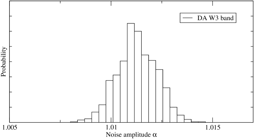
Figure 1.— Posterior distribution $P(\alpha|d)$ for the foreground-corrected W3 channel. This channel exhibits the strongest detection of $\alpha\neq 1$ of any DA.

Traditionally, the noise properties used in the Gibbs sampler (e.g., Eriksen et al., 2004) have been assumed known to infinite precision. In this paper, however, we relax this assumption, and introduce a new free parameter, $\alpha$, that scales the fiducial noise covariance matrix, $N^{\textrm{fid}}$,, such that $N=\alpha N^{\textrm{fid}}$. Thus, if there is no deviation between the assumed and real noise levels, then $\alpha$ should equal 1.

The full joint posterior, $P(s,C_{\ell},\alpha\,|\,d)$, now includes the amplitude $\alpha$. We can rewrite this as follows:

$$P(s,C_{\ell},\alpha\,|\,d)=P(d\,|\,s,\alpha)\cdot P(s,C_{\ell})\cdot P(\alpha)$$ (2)

where the first term is the likelihood,

$$P(d\,|\,s,\alpha)=\frac{e^{-\frac{1}{2}(d-s)(\alpha N)^{-1}(d-s)}}{\sqrt{|\alpha N|}},$$ (3)

the second term is a CMB prior, and the third term is a prior on $\alpha$. Note that the latter two are independent, given that these describe two a-priori independent objects. In this paper, we adopt a Gaussian prior centered on unity on $\alpha$, $P(\alpha)\sim N(1,\sigma_{\alpha}^{2})$. Typically, we choose a very loose prior, such that the posterior is completely data-driven.

The conditional distribution for $\alpha$ can now be expressed as

$$P(\alpha\,|\,s,C_{\ell},d)\propto\frac{e^{-\frac{\beta}{2\alpha}}}{\alpha^{n/2}}\cdot P(\alpha)$$ (4)

where $n=N_{\textrm{pix}}$ and $\beta=(d-s)N^{-1}(d-s)$ is the $\chi^{2}$. (Note that the $\chi^{2}$ is already calculated within the Gibbs sampler, as it is used to validate that the input noise maps and beams are within a correct range for each Gibbs iteration. Sampling from this distribution within the Gibbs sampler represent therefore a completely negligible extra computational cost.) For the Gaussian prior with unity mean and standard deviation $\sigma_{\alpha}$, we find that

$$P(\alpha\,|\,s,C_{\ell},d)\propto\frac{e^{-\frac{1}{2}(\frac{\beta}{\alpha}+\frac{(\alpha-1)^{2}}{\sigma_{\alpha}^{2}})}}{\alpha^{n/2}}$$ (5)

For large degrees of freedom, $n$, the inverse gamma function converges to a Gaussian distribution with mean $\mu=b/(k+1)$, where we have defined $k=n_{\textrm{pix}}/2-1$, and variance $\sigma^{2}=b^{2}/((k-1)(k-1)(k-2))$. A good approximation is therefore letting $\alpha_{i+1}$ be drawn from a product of two Gaussian distributions, which itself is a Gaussian, with mean and standard deviation

$$\mu=\frac{\mu_{1}\sigma_{2}^{2}+\mu_{2}\sigma_{1}^{2}}{\sigma_{1}^{2}+\sigma_{2}^{2}}$$ (6)

$$\sigma=\frac{\sigma_{1}^{2}\sigma_{2}^{2}}{\sigma_{1}^{2}+\sigma_{2}^{2}}.$$ (7)

This sampling step has been implemented in “Slave”, and we have successfully tested it on simulated maps. With $N_{\textrm{side}}=512$ and $l_{\textrm{max}}=1300$ and full sky coverage, we find $\alpha=1.000\pm 0.001$. Note that with such high resolution, the standard deviation on $\alpha$ is extremely low, and any deviation from the exact $\alpha=1.0$ will be detected.

3. Data

In this paper we analyze the 5-year WMAP data(Hinshaw et al., 2009), which is available from LAMBDA. We consider both the raw sky maps for each differencing assembly (DA), and the corresponding foreground-reduced maps (Gold et al., 2009). The nominal noise amplitudes are taken from the original 5-year data release as presented on LAMBDA. However, we note that after the initial publication of this paper, these have been corrected, as there was a discrepancy between the values presented on LAMBDA and those published in the WMAP Five Year Explanatory Supplement (Limon et al., 2009). The updated values agree very well with our results.

The foreground-reduced maps were produced from the raw maps by fitting and subtracting three fixed templates to each case. One of these templates was the (K-Ka) difference map, which mainly traces synchrotron, free-free and, possibly, spinning dust, and the other two were the H$\alpha$ template of Finkbeiner (2003) and the FDS8 thermal dust template of Finkbeiner et al. (1999). Here it is worth noting that the (K-Ka) difference map was smoothed to $1^{\circ}$ FWHM before fitting (Hinshaw et al., 2007); although this difference map is intrinsically noisy, it does not have power beyond $\ell\sim 400$, and, in effect, the raw and foreground-corrected maps are identical at high $\ell$’s. This will be explicitly demonstrated later.

In the low signal-to-noise regime, the estimated CMB signal will fluctuate greatly. In order to dampen the unruly behavior in this regime, we have chosen to bin the power spectrum for high $\ell$s. The $C_{\ell}$s are then generated from the binned signal power spectrum.

Unless explicitly noted, we apply the KQ85 WMAP sky cut (Gold et al., 2009), which removes 18% of the sky, including point source cuts. We also take into account the circular-symmetric beam profiles for each DA. Finally, the main analysis is carried out at a HEALPix resolution of $N_{\textrm{side}}=512$ and included harmonic space multipoles between $\ell=2$ and 1300. Including such high multipoles in the multipole expansion is acceptable in this case for two reasons; first, the WMAP beams fall off quickly in this regime, and the data becomes strongly noise dominated. Second, we bin the angular power spectrum heavily at high $\ell$’s.

4. Results

Table 1Noise estimation results

	$\alpha-1$ (in %)		$\sigma_{0}$ (mK)
Band	Direct	Bayesian	Nominal	Estimated	Updated
Raw maps
K1	$1.90$	$0.50$	$1.436$	$1.439$
Ka1	$0.10$	$0.10$	$1.470$	$1.471$
Q1	$0.23$	$0.15$	$2.254$	$2.256$
Q2	$0.16$	$-0.10$	$2.141$	$2.140$
V1	$0.08$	$-0.08$	$3.314$	$3.313$
V2	$-0.06$	$-0.03$	$2.953$	$2.953$
W1	$0.52$	$-0.37$	$5.899$	$5.889$
W2	$0.23$	$-0.43$	$6.565$	$6.550$
W3	$0.33$	$-0.30$	$6.926$	$6.916$
W4	$-0.45$	$-0.85$	$6.761$	$6.732$
Foreground-reduced sky maps
Q1	$0.83$	$0.51$	$2.2449$	$2.2542$	$2.254$
Q2	$0.87$	$1.02$	$2.1347$	$2.1455$	$2.141$
V1	$0.71$	$0.50$	$3.3040$	$3.3123$	$3.314$
V2	$0.63$	$0.62$	$2.9458$	$2.9549$	$2.953$
W1	$1.06$	$0.53$	$5.8833$	$5.8988$	$5.899$
W2	$1.27$	$0.71$	$6.5324$	$6.5555$	$6.565$
W3	$1.54$	$1.12$	$6.8849$	$6.9233$	$6.926$
W4	$0.04$	$-0.20$	$6.7441$	$6.7373$	$6.761$

Note. — Summary of 5-year WMAP noise amplitudes. Second column: Noise amplitudes estimated directly from high-$\ell$ power spectra, quoted in terms of $\alpha-1$ in percent. Third column: Noise amplitudes estimated by Gibbs sampling. The uncertainty on each of these numbers is $0.1\%$. Fourth column: Noise RMS per observation as quoted by the WMAP team on LAMBDA. Fifth column: Noise RMS per observation estimated by Gibbs sampling. sixth column: Noise RMS per observation as quoted by the WMAP team in the Five Year Explanatory Supplement, page 65.

The main results from our analysis are given in the third column of Table 1, where the posterior mean of $\alpha$ is given for each DA, both for raw and foreground-corrected maps. The numbers are quoted in terms of $\alpha-1$ in percent, and the corresponding posterior RMS is $0.1\%$.

For most of the raw DA sky maps, we find $\alpha=1$ to within a few sigma. The largest outlier is W4, with a negative amplitude of -0.85%. This DA is known to have the strongest correlated noise of any WMAP DA. In general, we find that the noise levels of the raw sky maps are in good agreement with the levels quoted by the WMAP team.

However, the situation is different for the foreground-corrected maps relative to the original noise amplitudes presented on LAMBDA. Specifically, in general the amplitudes of these maps are shifted high by $0.5-1.0\%$. The most extreme shift is seen for the W3 DA, with a posterior distribution centered on $\alpha=1.011\pm 0.001$.

With such significant discrepancies between the predicted and observed noise levels for the foreground-reduced sky maps, it should be possible to observe an absolute shift in the high-$\ell$ power spectra between simulated and the real sky maps. We therefore implemented a simple and approximate method to estimate $\alpha$ directly, without going through the Gibbs sampler: First, we calculate the angular power spectrum for each DA to high $\ell$’s, where the beam has killed all signal, and only noise is left. Any sky cut is ignored in this step. We then compute the average spectrum amplitude at $\ell>1300$, and define this as our noise amplitude estimate. Next, we simulate an ensemble of noise realizations from the RMS maps of each DA, and repeat the above calculation for each of these, and compute the corresponding average. The ratio between observed noise spectrum amplitude and the simulated average is then an estimate of $\alpha$, and can be compared to the values obtained from the Bayesian analysis. Again, note that this is only a rough cross-check on the our results, and should not be considered a proper stand-alone result because the sky cut is completely ignored.

The results from this exercise are tabulated in the second column of Table 1. In general, we see that these generally follow the same trends as those from the Bayesian analysis, although with systematically slightly higher amplitudes. This is likely due to neglecting of the galaxy cut, as foregrounds may obviously add to the total spectrum level.

In figure 2 we plot the power spectrum of the raw 5-year WMAP W3 sky map in $C_{l}$ units, together with the average W3 RMS $\sigma_{0}$ value, as given by the WMAP team. We also plot the estimated new W3 RMS, as estimated by Slave. Here it is clear that the Slave estimate fits the power spectrum better.

Finally, in Figure 3 we plot the same information, but to lower $\ell$’s and on a logarithmic scale. Notice how the high-$\ell$ W3 foreground reduced maps power spectrum equals the spectrum from the raw map. This implies that both the foreground-reduced and raw data have the same high-$\ell$ noise levels, and do not differ. We therefore conclude that the shift in the noise amplitude is not due to any shift in the actual data, but rather a difference in the WMAP5 noise models.

In the fourth column of Table 1, we tabulate for easy reference the noise RMS values for a single observations listed on LAMBDA. Here it is seen that the predicted noise levels for the foreground corrected maps is indeed lower than those for the raw maps. However, this does not seem to be the case, neither from looking at the raw power spectra, nor from the results from our Bayesian analysis.

Again, following the first publication of this letter, it was found that the foreground-correct noise RMS values on the LAMBDA website were not properly updated with the 5-year WMAP results. Therefore, the noise levels used in this analysis are known to be incorrect, and the reason is fully understood. Thus, this demonstrates the new method works well as the estimated values are fully consistent with the corrected 5-year values, shown in the sixth column of Table 1, column 6.

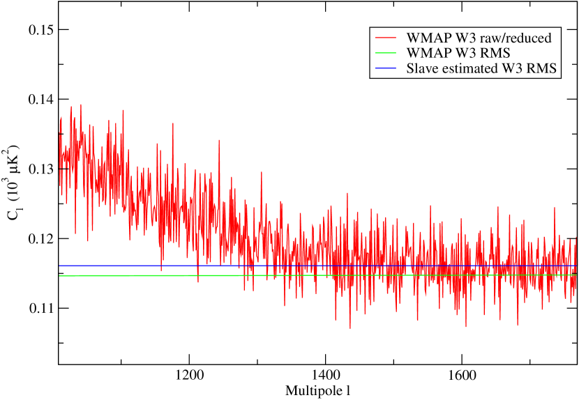
Figure 2.— The raw/foreground reduced power spectrum (red) plotted with the WMAP noise (green) and the Slave-estimated noise (blue). Note how Slave estimates a different noise level (blue) than the input noise level (green) .

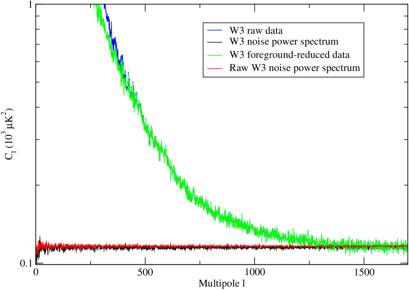
Figure 3.— A noise power spectrum realization for W3 RMS (black) and raw W3 RMS (red). The data power spectrum can be seen entering at high $\ell$ (blue and green), where the raw and foreground-corrected data converge.

5. Conclusion

We have introduced a new method for estimating white noise levels in CMB sky maps, using a Bayesian framework. We have then applied this method to the 5-year WMAP data, and re-estimated the noise levels of both the raw and foreground-reduced sky maps. In doing so, we found that the predicted noise levels for the raw maps are in acceptable agreement with the predictions, while the noise levels in the foreground-reduced maps are $0.5-1.0\%$ higher than the estimate initially provided by the WMAP team on LAMBDA.

The explanation for this effect has after the publication of this paper been found by the WMAP team simply to be an error in the results provided on LAMBDA: The quoted values were derived from the 3-year analysis instead of the 5-year analysis. However, the correct values were used in their cosmological analysis for the 5-year data, and no results are therefore compromised by this error.

Thus, the method has already been demonstrated to be both accurate and useful on a practical example. Further, it carries virtually no extra computational cost within a Gibbs sampler, since all required quantities are already computed within this algorithm. We therefore recommend this feature to be used as a standard part of the Gibbs sampling machinery, since it both provides additional robustness against noise mis-estimation, and also propagates the uncertainty in these estimates into the final CMB power spectrum.

Finally, we note that these noise estimates are very robust with respect to systematic issues such as foreground or CMB signal estimation. The reason is that the sky maps are well oversampled; with $\ell_{\textrm{max}}=1300$ there are $\sim 1.7$ million modes in the harmonic expansion, while at $N_{\textrm{side}}=512$ there are $\sim 3$ million pixels. Therefore, there are essentially 1.3 million modes available to estimate one single number, $\alpha$. If even greater precision is desired, one could simply consider increasing the pixel resolution one step further, which would leave the sky signal unchanged, because it is bandwidth limited, whereas the total number of modes in the map quadruples, thus decreasing the noise uncertainty.

References

- Bennett et al. (2003) Bennett, C. L., et al. 2003, ApJS, 148, 1
- Chu et al. (2005) Chu, M., Eriksen, H. K., Knox, L., Górski, K. M., Jewell, J. B., Larson, D. L., O’Dwyer, I. J., & Wandelt, B. D. 2005, Phys. Rev. D, 71, 103002
- Eriksen et al. (2004) Eriksen, H. K., et al. 2004b, ApJS, 155, 227
- Eriksen et al. (2007a) Eriksen, H. K., et al. 2007a, ApJ, 656, 641
- Eriksen et al. (2007b) Eriksen, H. K., Huey, G., Banday, A. J., Górski, K. M., Jewell, J. B., O’Dwyer, I. J., & Wandelt, B. D. 2007b, ApJ, 665, L1
- Eriksen et al. (2008a) Eriksen, H. K., Jewell, J. B., Dickinson, C., Banday, A. J., Górski, K. M., & Lawrence, C. R. 2008a, ApJ, 676, 10
- Eriksen et al. (2008b) Eriksen, H. K., Dickinson, C., Jewell, J. B., Banday, A. J., Górski, K. M., & Lawrence, C. R. 2008b, ApJ, 672, L87
- Finkbeiner et al. (1999) Finkbeiner D.P., Davis M., & Schlegel D.J. 1999, ApJ, 524, 867
- Finkbeiner (2003) Finkbeiner, D. P. 2003, ApJS, 146, 407
- Gold et al. (2009) Gold, B., et al. 2009, ApJS, 180, 265
- Górski et al. (2005) Górski, K. M., Hivon, E., Banday, A. J., Wandelt, B. D., Hansen, F. K., Reinecke, M., & Bartelmann, M. 2005, ApJ, 622, 759
- Groeneboom & Eriksen (2009) Groeneboom, N. E., & Eriksen, H. K. 2009, ApJ, 690, 1807
- Groeneboom (2009) Groeneboom, N. E. 2009, arXiv:0905.3823
- Guth et al (1981) Guth, A. H, 1981, Phys. Rev. D, 347
- Hinshaw et al. (2007) Hinshaw, G., et al. 2007, ApJS, 170, 288
- Hinshaw et al. (2009) Hinshaw, G., et al. 2009, ApJS, 180, 225
- Jewell et al. (2004) Jewell, J., Levin, S., & Anderson, C. H., 2004, ApJ, 609
- Larson et al. (2007) Larson, D. L., Eriksen, H. K., Wandelt, B. D., Górski, K. M., Huey, G., Jewell, J. B., & O’Dwyer, I. J. 2007, ApJ, 656, 653
- Limon et al. (2009) Limon, M. et al. 2009, Wilkinson Microwave Anisotropy Probe (WMAP): Five–Year Explanatory Supplement, Greenbelt, MD: NASA/GSFC
- Linde et al. (1982) Linde, A. D., 1982, Phys. Lett. B 108, 389
- Linde et al. (1983) Linde, A. D., 1983, Phys. Lett. B 155, 295
- Linde et al. (1994) Linde, A. D., 1994, Phys. Rev. D49, 748
- Mukhanov et al. (1981) Muhkanov, V. F., Chibishov, G. V., & Pis’mah Zh. 1981, Eskp. Teor. Fiz. 33, 549
- O’Dwyer et al. (2004) O’Dwyer, I. J., et al. 2004, ApJ, 617, L99
- Ruhl et al (2003) Ruhl et al., 2003, ApJ599, 786
- Runyan et al. (2003) Runyan et al., 2003, ApJ, J. Suppl. Ser. 149, 265
- Scott et al. (2003) Scott et al., 2003, MNRAS341, 1076
- Smoot et al. (1992) Smoot et al., 1992, ApJ396, L1
- Starobinsky et al (1982) Starobinsky, A. A., 1982, Phys. Lett. B 117, 175
- Wandelt et al. (2004) Wandelt, Benjamin D. and Larson, David L. and Lakshminarayanan, Arun Phys. Rev. D70,8