Fitting the Phenomenological MSSM
Abstract:
We perform a global Bayesian fit of the phenomenological minimal supersymmetric standard model (pMSSM) to current indirect collider and dark matter data. The pMSSM contains the most relevant 25 weak-scale MSSM parameters, which are simultaneously fit using ‘nested sampling’ Monte Carlo techniques in more than 15 years of CPU time. We calculate the Bayesian evidence for the pMSSM and constrain its parameters and observables in the context of two widely different, but reasonable, priors to determine which inferences are robust. We make inferences about sparticle masses, the sign of the parameter, the amount of fine tuning, dark matter properties and the prospects for direct dark matter detection without assuming a restrictive high-scale supersymmetry breaking model. We find the inferred lightest CP-even Higgs boson mass as an example of an approximately prior independent observable. This analysis constitutes the first statistically convergent pMSSM global fit to all current data.
CERN-PH-TH/2009-037
1 Introduction
There is currently an expectation that with the start of the Large Hadron Collider (LHC), high energy physics will soon enter a new phase highly dominated by new data that could imply physics beyond the Standard Model (SM). Over the past years, low energy supersymmetry (SUSY) has become the standard approach to study the potential physics beyond the SM, mostly because of its natural power to address the hierarchy problem. The Lagrangian parameters of the minimal supersymmetric extension of the SM (for a recent review, see [1]) makes its phenomenological study impractical. It may well be that the mechanism that mediates SUSY breaking to the observable sector provides relations between many of these parameters. Unfortunately, however, there are many different mediation mechanisms in the literature, with no one clearly preferred.
In order to extract computable information, many works have reduced the number of parameters by truncating to a handful of soft-breaking parameters at a high energy scale. The remaining set of parameters are used as boundary conditions for renormalisation group equations (RGE), which are run down to the weak-scale. A large amount of minimal supersymmetric standard model (MSSM) based studies have been carried out in the way described above. Most of them were performed in the context of the constrained MSSM (CMSSM, also sometimes called mSUGRA for minimal supergravity) set-up which have only independent non-SM parameters (and a sign choice). Many groups have been pursuing a programme to fit this model and identify regions in parameter space that might be of interest with the forthcoming LHC data. See for instance [2, 3, 4, 5, 6, 7]. Complete scans over up to free parameters of CMSSM with a combined treatment of likelihoods from different experimental constraints were possible with Markov Chain Monte Carlo (MCMC) sampling techniques [5, 8, 9, 10, 11, 12, 13, 14]. However, the truncation to a handful of parameters in the CMSSM, is at best a very strong assumption, and most likely over-restrictive.
There are two directions that can be followed to properly study low-energy supersymmetric models. The top-down approach has been tried over the years by deriving the otherwise free parameters from an ultraviolet extension of the MSSM. Models of unification, different sources of SUSY breaking, such as gravity and gauge mediation and classes of string compactifications [15, 16, 17, 18, 19, 20, 21, 22, 23] have been used to provide high energy expressions for the soft breaking parameters. Soft SUSY breaking terms can be computed at energies as high as the GUT scale of GeV, and renormalisation group running to the TeV scale allows contact to be made with potential quantities of interest such as sparticle masses. Recent progress in moduli stabilisation in string theory has made this approach more concrete and calculable with explicit results for some classes of models. This is very encouraging but usually the string derived models fill only a small subset of the full CMSSM parameter space, which could make them impossible to differentiate from the CMSSM. The proliferation of SUSY breaking mechanism set-ups mean that analyses where only one is picked tend to be very specific, with a rather limited range of applicability. It is desirable to side-step such extreme model dependence with a different approach.
Alternatively, one can use a bottom-up approach to low-energy SUSY. In this case the soft breaking parameters are considered at the SUSY scale without referring to their high energy origin. All the parameters can in principle be varied over the experimentally allowed range and compared with potential observations at the LHC and other experiments. It is a formidable task to consider all the 124 parameters, due mostly to computing limitations. An interesting compromise is the pMSSM [24] which we consider here. In this model, the number of free parameters is 20 soft-breaking parameters (and a parameter) plus 5 SM ones and are selected by the requirements of consistency with unobserved flavour changing and CP violating processes. However, even this simplified version of the MSSM requires a lot of computer power to be analysed in and details. The ability of future collider measurements to constrain the pMSSM has been estimated using MCMC methods in Refs. [25, 26].
At present, SUSY forecasts for the LHC necessarily contain large uncertainties. In particular, there is a strong model dependence on the mechanism for SUSY breaking. Realistic predictions need guidance from direct and precise (collider and other related) experimental data. Interestingly, the converse is also very important: the experiments need unbiased phenomenological guidance about the expected nature or properties of SUSY. This is what we aim to accomplish, eventually.
The purpose of this article is to perform a global fit of the pMSSM and make SUSY forecasts for collider and dark matter search experiments using Bayesian statistics methods. For given prior probability and likelihood densities, Bayes theorem provides the way to extract the posterior probability density for the parameters. It can also be used for model comparison when enough data is available. This formalism has been used in many fields of science, including cosmology (see [27, 28] for recent reviews). Markov Chain Monte Carlo (MCMC) and related techniques have recently begun to be used to perform Bayesian inference on supersymmetric models. The increasing access to large scale computing power and improved methods of calculation are making these techniques more manageable with time and we have been able to tackle the relevant parameters of the pMSSM.
The complete and simultaneous scan of the 25 parameters and a sign111Where we refer to 25 parameters, we shall really mean 25 continuously varying parameters plus the one discrete sign choice. for the pMSSM construction was performed using the MultiNest program [29, 30]. At the heart of the algorithm is the nested sampling technique [31] that revolutionised computational Bayesian inference by prioritising a computation of the Bayesian evidence rather than solely on computing the posterior probability distribution function (PDF) of model parameters (although the latter is obtained at no additional cost), as is the case in traditional Monte Carlo algorithms (e.g. MCMC). We will review the nested sampling method in an appendix. In simple terms, similar to the MCMC, nested sampling is an iterative Monte Carlo method that, starting with a relatively small number of points (a few thousand in our case), it produces a list of a large number of points ( in our case) ordered in increasing likelihood. We used it here because it computes both the evidence and the posterior PDF, as opposed to traditional MCMC methods which only calculate the posterior PDFs. Further the MultiNest algorithm is efficient in handling complicated problems with multimodal/degenerate posterior distributions.
We emphasise that the current situation with no direct sparticle measurement data yet from LHC makes the issue of prior dependence critical. For this reason, it is expected that extraction of prior independent information of our analysis will be difficult. Interestingly, however, we find some results with approximate prior independence. In order to illustrate the issue of prior dependence of results we consider priors that are flat in the parameters themselves (‘linear’) and flat in the logarithm of the parameters (‘log’) priors. As usual in Bayesian statistics prior dependence should not be understood as a drawback but as a positive feature that can be used to determine when enough data is available to unambiguously make inferences. It is expected that, if SUSY is discovered, the addition of LHC sparticle mass data will relax any prior dependence, and so an analysis along the lines of ours could be used to extract prior independent information.
The amount of work related to this project required very efficient algorithms and access to high performance computing. We used the University of Cambridge supercomputers: COSMOS from the Department of Applied Mathematics and Theoretical Physics (DAMTP) and the Darwin cluster from the High Performance Computing Service (HPC). The final run was made in terms of 60 12-hour jobs, each corresponding to a cluster of 128 CPUs on HPC and 40 8-hours jobs, each corresponding to a cluster of 64 CPUs, on COSMOS (making a total of more than 15-year standard CPU time). Some results of a complete and independent (from the one we present here) runs with fewer experimental constraints were presented by one of us (SSA) at the SUSY 2008 conference and reported in Ref. [32]. While we were upgrading our analysis, a study of randomly scanned pMSSM points appeared [33], similar in philosophy to Ref. [4]. In the conclusions, we contrast the aims and methodologies of our work with these.
In order to make a self-contained presentation we briefly describe Bayesian inference and relevant terminologies in Section 2. We construct the elements needed for inference in the context of the pMSSM in Section 3. The experimental constraints or observables used are described in Subsection 3.2. The sampling procedure and the different high energy physics software used to predict the observables are presented in Subsection 3.4. In Sections 4 and 5 we analyse our results and then conclude. In the Appendix we briefly review the nested sampling method and how the MultiNest program works.
2 Bayesian Inference
Bayesian inference fits and plays an important role in the scientific process of data collection and modelling. It particularly deals with the steps that involve model fitting to data and the technique of assigning preferences to alternative models (model comparison). This subject is very important especially with the imminent start of the LHC experiments. Here we will give a short review of the basics of Bayesian statistics that are useful in our work.
2.1 Bayes’ theorem
Consider a given model or hypothesis (we shall take to be the pMSSM) defined by some set of parameters (in our case, 25 parameters) . We wish to know the PDF of the parameters given the data and the model set-up, . , being the parameters’ PDF after confrontation with data, is called the posterior PDF. The likelihood, is a measure of how well a model point predicts data set . In order to calculate the posterior from the likelihood, one must assign some prior PDF to the parameters to parametrise our uncertainty in them before the model is confronted with data. Bayes’ theorem then describes how one may obtain the posterior from the other two PDFs and a normalisation constant , the Bayesian evidence for the model in light of the data:
| (1) |
The Bayesian evidence is given by
| (2) |
Here is the dimensionality of the parameter space; for the pMSSM. Since the Bayesian evidence does not depend on the parameter values , it is usually ignored in parameter estimation problems and posterior inferences are obtained by exploring the un–normalised posterior using standard MCMC sampling methods. However, the evidence plays a central role in our discussion.
A useful feature of Bayesian parameter estimation is that one can easily obtain the posterior PDF of any function, , of the model parameters . Since,
| (3) |
where the probability chain rule is employed for the second equality and is the Dirac delta function. Thus one simply needs to compute for every Monte Carlo sample and the resulting sample will be drawn from . We make use of this feature in Sections 4 and 5 where we present the posterior probability PDFs of various observables used in the analysis of the pMSSM.
Before proceeding to discuss prior distributions, we first briefly address 222We follow the description in:http://www.dsg.port.ac.uk/ valiviitaj/Lectures2006/CrittendenCMB2003.pdf, the difference between the Bayesian and the frequentist approaches to inference. Bayesian inference (using Bayes’ theorem) is a robust technique for updating prior knowledge or belief based on new data. It is unlike the frequentist approach where observations are viewed as random draws from some pool of possible observations such that the probability of an observation is the frequency observed with a large number of repeated measurements. Frequentists usually focus on the likelihood and argue that the Bayesian approach is too subjective because of the use of priors. Bayesians reply that when many examine frequentist statistics, they are actually implicitly using priors anyway. If one thinks of a region of parameter space with the lowest chi-squared values as being more likely than a region of parameter space with much higher chi-squared values, one is implicitly using some vague prior. The two approaches are asking different questions. Bayesians ask, “how likely is a given parameter value given the data?”, while frequentists ask, “how probable is the data, given certain parameters?” In situations where the data is very informative the two approaches give the same results. We are interested in PDFs of parameters and so we use Bayesian statistics. By comparing results from different but reasonable priors, we obtain an estimate of how robust an inference is given current data.
2.2 Priors
The prior probability of the model parameters is a PDF that gives a subjective measure of our initial knowledge/ignorance about the values of the parameters of the model before the data are taken. Symmetries and physical observations or expectations are usually a good guide to which priors to take. Information theory also provides a way of selecting priors by favouring those that maximise the entropy of the distributions. Some commonly used prior PDFs are:
| (4) | |||||
| (5) | |||||
| (6) |
The linear priors are often used for translational (like time and location) parameters, where there is no information to suggest that one value is preferred over others. The Jeffreys prior, also referred to as logarithmic (log) prior, is uniform in the logarithm of the parameter. These two priors are improper since they diverge when integrated over an infinite range. Our log and linear priors will be bounded by the requirements of perturbativity of the model, by passing previous direct sparticle search constraints and by the requirement of not too large fine-tuning in the Higgs potential parameters. These three criteria are sufficient to bound all 20 non-SM input parameters to a finite range. The Gaussian prior, on the other hand, is proper and integrable but requires previous experimental knowledge on and . This is indeed the case for our 5 SM input parameters, and we use Gaussian priors for them (see Section 3.1).
Assuming the parameters are independent, the resultant prior is obtained by the product of all the prior probability densities for each of the individual parameters. For instance, in the case of pMSSM with parameters, ,
| (7) |
For our construction and analysis we are going to choose a linear prior measure for the pMSSM parameters described in Section 3.1. This is because there are no observational evidence that hint to giving preference of some parameter region over others. We are going to determine bounds on the parameters from the fact that the parameter values have to be not far away from the TeV-scale in order avoid the little hierarchy problem. We are going to call such case/scenario as the linear prior. We then check the dependence of the results in our analysis on prior change by performing another analysis with a log prior. When we refer to a log prior, in fact the Jeffreys prior is only used for all parameters which only have positive bounds. Parameters which are allowed to take either sign present a problem with Jeffreys priors since the prior diverges at the origin. Therefore, the priors of such parameters are always taken to be linear.
For parameter estimation, the priors become irrelevant once the data employed are powerful enough. This is already in evidence by comparing Bayesian CMSSM fits [34] with those in similar supersymmetric models which have a lower number of free parameters, for example the large volume string compactification (LVS) scenario [23]. The LVS scenario has two less free parameters than the CMSSM and current indirect data are already enough to make the result approximately prior independent. We may expect the addition of two precise, constraining, non-degenerate measurements (such as sparticle mass measurements from the LHC) to have the same effect upon the CMSSM.
For model comparison, the dependence on priors always remains (although with more informative data the degree of dependence on the priors is expected to decrease, see e.g. [27]). Indeed this explicit dependence on priors is one of the most attractive features of Bayesian model selection. Refs. [13, 35] identified prior distributions in high-scale CMSSM Lagrangian parameters. In particular, a Jacobian was defined to transform between derived parameters (such as ) and more fundamental Lagrangian parameters from which they are derived. It is not our purpose here to find the ‘most natural’ prior because any such choice is necessarily subjective. Instead, we shall check the robustness of any inference under a reasonable variation of the priors. Such a check is especially required in model comparison hypothesis tests, which may be particularly sensitive to the particular choice of prior and its associated metric in parameter space [36].
2.3 Model comparison
In order to evaluate and rank two alternative models and in the light of data one needs to compare their respective posterior probabilities given the observed data set , as follows333Here we follow the description by [37].: use Bayes’ theorem to relate the plausibility of given the data, , to the predictions made by the model about the data, , and the prior plausibility of , . With this procedure one could construct the following probability ratio
| (8) |
is the prior probability ratio for the two models, it measures how much our initial beliefs favour over . It is often set to unity but may occasionally require further consideration. The other ratio, measure how well the observed data were predicted by and . It can be seen from 8 that the Bayesian evidence takes the centre stage in Bayesian model comparison. As the average of likelihood over the prior, the Bayesian evidence is higher for a model if more of its parameter space is likely over some region of significant integrated prior (‘prior mass’) and smaller for a model with highly peaked likelihood but has a large prior mass associated with low likelihood values. Hence, Bayesian model selection automatically implements Occam’s razor, since the prior PDF decreases for models with higher numbers of parameters. A more complicated theory will only have a higher evidence if it is significantly better at explaining the data than a simpler theory with less parameters. This technique was applied in [34] to compare two CMSSM models: versus . We shall perform a similar comparison for the pMSSM in Subsection 4.4. The comparison of different GUT scale SUSY breaking models is also interesting [38].
Another perspective on model comparison is in quantifying the consistency between two or more data sets or constraints [39, 40]. Different experimental constraints may ‘pull’ the model parameters to different directions and consequently favour different regions of the parameter space. Any obvious conflicts between the observables are likely to be noticed by the ‘chi by eye’ method commonly employed to-date, but it is imperative for forthcoming high–quality data to have a method that can quantify such discrepancies. The simplest method for analysing different constraints on a particular model is to assume that all constraints and data provide information on the same set of parameter values. This can be considered as one hypothesis or model, . This is the assumption which underlies the joint analysis of the constraints. However, if we are interested in accuracy as well as precision then any systematic differences between constraints or data should also be taken into account. In the most extreme case they could be in conflict to the extent that each of them would require its own set of parameter values, since they are in different regions of parameter space. This scenario can be considered as another hypothesis or model, , to be compared with the other, . Bayesian inference provides a very easy method of distinguishing between the scenarios and . This technique was illustrated in Refs. [34, 41] by examining the compatibility between branching ratios and the anomalous magnetic moment of the muon in the CMSSM.
The natural logarithm of the ratio of posterior model probabilities provides a useful guide to what constitutes a significant difference between two models:
| (9) |
In Tab. 1 we summarise the conventions we use in this paper to separate between different levels of evidence.
| Odds, | Probability | Remark | |
|---|---|---|---|
| Inconclusive | |||
| Weak Evidence | |||
| Moderate Evidence | |||
| Strong Evidence |
The evaluation of the multi-dimensional integral (2) is a challenging numerical task. Standard techniques like thermodynamic integration [42] are extremely computationally expensive which makes evidence evaluation typically at least an order of magnitude more costly than parameter estimation. Some fast approximate methods have been used for evidence evaluation, such as treating the posterior as a multivariate Gaussian centred at its peak (see e.g. [39]), but this approximation is clearly a poor one for multi–modal posteriors (except perhaps if one performs a separate Gaussian approximation at each mode). The Savage–Dickey density ratio has also been proposed [43] as an exact, and potentially faster, means of evaluating evidences, but is restricted to the special case of nested hypotheses and a separable prior on the model parameters. Bridge sampling [44, 45, 46] allows the evaluation of the ratio of Bayesian evidence of two models and was implemented in fits to the CMSSM in Ref. [10]. Bank sampling [47] (a particular implementation of the MCMC technique) also allows evidence ratios to be calculated with half the number of points than required for bridge sampling, and was used in CMSSM fits in Ref. [13]. It is not yet clear how accurately bank sampling can calculate these evidence ratios, and both bridge and bank sampling have the disadvantages of only being able to calculate evidence ratios, not the evidence itself. When comparing models, this introduces an inefficiency of a factor of compared to the latter case. Various alternative information criteria for model selection are discussed by [28], but the evidence remains the preferred method.
The nested sampling approach, introduced by Skilling [31], is a Monte Carlo method targeted at the efficient calculation of the evidence. It also produces posterior inferences as a by–product. Feroz & Hobson [29, 30] built on this nested sampling framework and have recently introduced the MultiNest algorithm which is efficient in sampling from multi–modal posteriors exhibiting curving degeneracies, producing posterior samples and calculating the evidence value and its uncertainty. This technique has greatly reduced the computational cost of model selection and the exploration of highly degenerate multi–modal posterior PDFs. We employ this technique in this paper.
3 The pMSSM
The MSSM Lagrangian has the form where contains all of the kinetic terms, gauge and Yukawa interactions while preserving SUSY invariance. It is based on the gauge group and superpotential, , constructed with a particle content in the following chiral superfields shown with their corresponding charges:
| (10) |
The superpotential is given by
| (11) |
Here we use the convention in [48] and denote the colour index of the fundamental representation by ; the fundamental representation indices by and the generation indices by is the totally antisymmetric tensor, with .
The soft SUSY-breaking part of the Lagrangian consists of different mass and coupling terms:
| (12) |
where the part including the SUSY breaking sfermion masses is
| (13) | |||||
Each mass parameter in Eq. 13 is a hermitian matrix in generation space.
| (14) |
gives the SUSY breaking higgs masses and bi-linear coupling terms. The SUSY breaking scalar trilinear couplings are
| (15) |
where fields with a tilde represent the scalar components of the corresponding capital letter superfield and the soft SUSY-breaking A-terms, each a complex matrix in generation space, are defined (no summation on is inferred) as
| (16) |
Finally, writing the bino as , as the unbroken- gauginos and as the gluinos, then the gaugino-mass part of the Lagrangian is
| (17) |
The parameters together make a total of free parameters in , before re-phasing and higgs potential minimisation [49, 50, 24]. In the CMSSM, the SUSY breaking scalar masses the gaugino masses and trilinear couplings are collapsed to the flavour independent parameters , and respectively, at grand unification scales GeV. and are related to the boson mass through higgs potential minimisation conditions. and , the ratio of the Higgs vacuum expectation values (vevs) remain as free parameters. However in this paper we instead explore the parameters at the weak-scale in its phenomenologically most relevant directions and following Ref. [51] call the set-up the pMSSM. In Subsection 3.1 we describes how the parameters in the pMSSM set-up are derived from the much larger parameter space of the parent MSSM.
3.1 Parameters
Sources of CP-violation in the MSSM are tightly constrained by experimental limits on the electron and neutron electric dipole moments and from results on K-meson system experiments. Assuming that the MSSM soft SUSY-breaking parameters are real is consistent with such tight bounds, indeed significant departures from this assumption usually require a specific cancellation or suppression mechanism in order to pass the constraints. To suppress flavour changing neutral current (FCNC) processes, all off-diagonal elements in the sfermions masses and trilinear couplings are set to zero and the first and second generation soft terms are set to be equal. , , may all change the likelihood significantly, and we also include because it is relevant for the computation of the anomalous magnetic moment of the muon [52]. We set since these are proportional to the SM Yukawa couplings which are very tiny and so they will have negligible effect on the likelihood. All the other trilinear couplings are set to zero. Our Higgs-sector parameters are specified by , and as discussed above, we must add and to the list of parameters.
All of the parameters mentioned so far are purely non-SM. However, some of the SM parameters significantly affect the likelihood. The relevant SM parameters include the electromagnetic coupling constant and the strong coupling constant . The values of these two couplings are taken at the -boson pole mass energy scale evaluated in the renormalisation scheme. The tau lepton mass and , the Fermi constant have been so precisely determined that their uncertainty has negligible error on the likelihood and so they are fixed at their global average values: GeV and GeV-2[53]. The top and bottom quark masses are not as precisely known and can have significant effects on predictions of supersymmetric models. They are therefore included as parameters with, using the experimental measurements of their central values and uncertainties, Gaussian priors. Despite the fact that the -boson mass, , is precisely determined, we include its uncertainty because one of the observables used for the analysis (the total decay width of the -boson ) is proportional to and the pMSSM predicted values can fall outside the expected experimentally determined range with a sigma variation in . So adding the SM parameters,
| (18) |
makes a total of continuously varying parameters in the pMSSM. These are listed together with their ranges or Gaussian prior distributions in Tab. 2. These pMSSM directions make up its parameter-space. Our aim is to eventually construct a detailed map of the parameter-space that could be of help to or guide for collider and other SUSY-related experiments. In Subsection 3.2 we briefly describe the observables considered and summarise the experimental constraints coming from each.
| Parameter | Description | Prior range |
|---|---|---|
| Bino mass | [ TeV, TeV] | |
| Wino mass | [ TeV, TeV] | |
| Gluino mass | [ TeV, TeV] | |
| 1st/2nd generation slepton | [ GeV, TeV] | |
| 3rd generation slepton | [ GeV, TeV] | |
| 1st/2nd generation slepton | [ GeV, TeV] | |
| 3rd generation slepton | [ GeV, TeV] | |
| 1st/2nd generation squark | [ GeV, TeV] | |
| 3rd generation squark | [ GeV, TeV] | |
| 1st/2nd generation squark | [ GeV, TeV] | |
| 3rd generation squark | [ GeV, TeV] | |
| 1st/2nd generation squark | [ GeV, TeV] | |
| 3rd generation squark | [ GeV, TeV] | |
| Trilinear coupling for top quark | [- TeV, TeV] | |
| Trilinear coupling for b-quark | [- TeV, TeV] | |
| Trilinear coupling for -quark | [- TeV, TeV] | |
| Trilinear coupling for -quark | [- TeV, TeV] | |
| up-type Higgs doublet mass | [ GeV, TeV] | |
| down-type Higgs doublet mass | [ GeV, TeV] | |
| scalar doublets vevs ratio | [2, 60] | |
| top quark mass [54] | 172.6 1.4 | |
| Z-boson mass | 91.187 0.021 | |
| b-quark mass | 4.20 0.07 | |
| 1/ | electromagnetic coupling constant | 127.918 0.018 |
| strong coupling constant | 0.117 0.002 |
3.2 Observables and experimental constraints
The SM fits high precision electroweak data well [55]. However, on the one hand, there are some observables whose SM predicted values significantly differ from the corresponding experimental indications. The discrepancies could be explained by the direct or indirect presence of supersymmetric particles (or sparticles) in the interactions. On the other hand the very precise agreement between the SM prediction and the experimentally determined values of some other set of observables could be altered by the presence of non-SM particles. The absence of any significant such deviation puts tight constraints on possible new physics beyond the SM (SUSY in our case); see for instance [56, 57] and references therein. The values of the sparticle masses affects these tendencies. For instance, the effect of sparticles in loop corrections to electroweak physics observables (EWPO) decouple if their masses are much heavier than (300 GeV and above according to Ref. [58]). Lighter sparticles with masses just above current experimental limits will alter the agreement between the electroweak data and SM predictions – hence the preference for low energy (weak-scale) SUSY.
For the pMSSM set-up we use observables and constraints from high precision collider measurements that are sensitive to effects of new physics via virtual loops. These include five EWPO: the -boson mass, , the effective leptonic weak mixing angle, , the total -boson decay width, , the anomalous magnetic moment of the muon, and the mass of the lightest MSSM Higgs boson, ; five B-physics observables: branching ratios , , , and the mass-mixing parameter ; and the cosmological observable, dark matter relic density from WMAP5 results. We next briefly describe each of these physical observables and state the corresponding experimental constraints. We first discuss constraints from EWPO and end the Section with discussion of sparticle mass limits.
-
•
-boson mass, :
The CDF Run II electroweak public results cited the -boson mass measurement as the single most precise measurement to date and quotes [59](19) Theoretically the mass can be calculated from
(20) where is the fine structure constant at the renormalisation energy scale, is the Fermi weak coupling constant and includes all radiative corrections to the mass (see e.g. [60, 61] and references therein). The high precision in this measured quantity constrain any radiative corrections from new physics effects. The experimental precision is very high to the extent that measurements can be sensitive even to two-loop effects involving sparticles. We include a theoretical uncertainty of 10 MeV on by adding it in quadrature with the experimental uncertainty. We use SUSYPOPE [62, 63] to calculate the -boson mass and the other EWPO. The most complete available SM two loop corrections and the dominant results for two loop SUSY corrections as implemented in SUSYPOPE currently give the most accurate predictions within the MSSM.
-
•
-boson decay width, :
The partial -boson decay width in the massless fermion limit () is given by [64](21) where are the neutral weak coupling constants modified to include electroweak (EW) radiative effects, parametrises the QCD corrections and includes some non-factorisable EW contributions. The colour factor is 1 for leptons and 3 for quarks. The current experimental value for the total decay width is [59]
(22) Theoretically
(23) where are the decay widths into SM leptons and quarks. is for the decays into invisible particles (neutrinos and possibly, if they are light enough, neutralinos). Supersymmetric contributions enter via virtual corrections to the partial decay widths into lepton and quarks.
-
•
Effective mixing angle, :
The effective electro-weak mixing angle depends only on the ratio of the effective weak couplings(24) for the vertex that couples the -boson and leptons in the Lagrangian: . It is determined from various asymmetry measurements around the -boson peak from colliders after removing QED effects [65]. We use the experimental estimate [59]
(25) -
•
Z-pole asymmetry parameters from processes:
The results from the LEP and SLC colliders on Z-boson properties (its mass, partial and total widths, and couplings to fermion pairs) are in good agreement with the SM predictions [65]. The precision is high enough to probe loop-level predictions where both SM and beyond the SM corrections are absorbed into effective coupling constants. The LEP data consist of hadronic and leptonic cross sections, leptonic forward-backward asymmetries, polarisation asymmetries, and partial widths and forward-backward asymmetries. The Z-boson parameters derived from the data which we employ for our analysis include the ratios (which we assume to be the average of , and ), and . These are defined as(26) and are constrained to be
The Z-boson interacts with fermions through a mixture of vector and axial-vector couplings. This makes the strength of the interaction between left- and right-handed fermions unequal and leads to the production of polarised Z-bosons at the colliders. As result there are measurable asymmetries (such as a forward-backward asymmetry) in the angular distributions of the final-state fermions . The forward-backward asymmetry is related to the probability that the travels in the same (forward) or opposite (backward) direction to the incident direction and is quantified by
(27) where is the cross section in the forward(backward) directions. In terms of the effective vector and axial-vector neutral current couplings, and respectively, other Z-pole asymmetries are:
(28) Here gives a measure of the asymmetry for the different possible final state fermions. At LEP the Z-pole forward-backward asymmetries and were precisely measured for the final states and respectively. We impose and for our analysis.
Using polarised beams, the SLD experiment made a direct and precise measurement of the parameter from the left-right asymmetry
(29) were and are the production cross sections for Z bosons produced with left- and right-handed electrons respectively. The same parameter, , is also indirectly constrained by LEP experiments. Using the measurements of the parameters and can then be inferred from measurements at LEP. Hence, the LEP and SLC results form a complete set of the parameter measurements. The asymmetry parameter constraints we use are , and .
-
•
Muon anomalous magnetic moment, :
The world average for the muon anomalous magnetic moment as determined from hadrons-based experiment at Brookhaven [66] is . Other results from experiments based on the lepton decay to hadrons [67, 68, 69] differ slightly and we are not using those here444See [70] for a recent review.. The experimental results are around deviation from the SM prediction [71] giving(30) SUSY is a good new physics candidate that can explain this deviation. For sparticles all of mass , their contribution to is of order [72]
(31) We use micrOMEGAs [73, 74, 75, 76] to predict , correcting it with , which includes contributions from the dominant QED-logarithmic piece, some dominant two-loop corrections [70] and the recently computed -enhanced term (see [77] and references therein)
(32) For our analysis we add in quadrature a theoretical error of to the error above and use the average value .
-
•
Lightest Higgs boson mass, :
The SM higgs mass is constrained to GeV by LEP direct search experiment (see e.g. [78] and references therein). The predicted higgs mass can be parametrised by , the ratio of the MSSM higgs coupling to two neutral -bosons to the equivalent SM coupling. In the MSSM so we use the above LEP mass limit for and use the MSSM higgs mass limit for . -
•
Branching ratio ():
The experimental value of the decay rate of the flavour changing process agrees to high precision with the SM prediction. This stringently constrains new physics models that may contribute to the process. For SUSY the leading contributions come from loops with charged Higgs bosons (these interfere constructively with the SM contributions) and charginos. Loops with neutralinos are small (see for instance, [79]). A recent theoretical estimate for the SM contribution to the branching ratio of which we call at next-to-next-to leading order (NNLO) in QCD is [80, 81, 82, 83] , where a 1.6 GeV lower energy cut is applied to the photon. The central value is lower than a world-average experimental value from the Heavy Flavor Averaging Group [84] (HFAG)555We note that the most recent central value has shifted slightly to 3.52: this small change would leave no significant imprint on our fits.(33) The values predicted for this observable at different parameter points are constrained by combining in quadrature the experimental and SM prediction errors:
(34) The branching ratio therefore constrains non-SM contributions. We use SuperIso2.0 [85] to predict the MSSM plus SM branching ratio666The program SusyBSG [86] now contains a more accurate prediction of this branching ratio to two-loops in MSSM parameters. It could lead to an estimated shift in the predicted branching ratio of , which may be considered to be included within our estimate of theoretical error..
-
•
Branching ratio ():
The branching fraction for the flavour changing process is predicted to be within the SM [87]. In the MSSM, interactions involving neutral Higgs bosons can enhance the branching fraction by several orders of magnitude at high . The branching ratio is experimentally bounded from above by recent CDF II results, implying(35) at CL [88]. We apply a continuous likelihood constraint derived from CDF II data upon the MSSM prediction [89]. The resulting penalty is shown in Fig. 1.
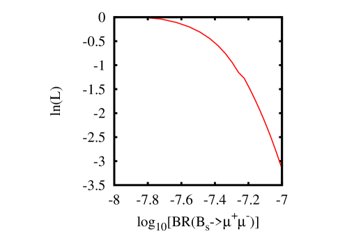
Figure 1: Likelihood penalty on the predicted value of . -
•
- mass difference, :
The neutral -meson oscillates between particle and antiparticle states via flavour changing processes. The frequency of oscillation is proportional to the mass difference It has been measured to be [90]. Its SM prediction can be obtained from an overall unitarity triangle fit: [91]. We use the ratio of the experimental constraint to the SM prediction(36) to constrain the predicted frequencies. Our pMSSM predicted values are based on the results in [92] and references therein:
where are the bottom- and strange-quark masses evaluated at the scale ;
(38) are the effective couplings that parametrise the correction to the down-type Yukawa couplings,
(39) is the supersymmetric Higgs mass terms and is the trilinear soft breaking term involving the stops. is given by
-
•
Branching ratio :
The purely leptonic decay proceeds via the annihilation of - and -quarks into . The SM prediction for the branching ratio of the process is given by(40) where and are the meson and pole masses, respectively, and is the -meson lifetime. For the SM prediction we use the average of the result from unitarity triangle fits () and the result obtained from the experimental determination of and () 777See “New Constraints from B and K rare decays” at http://www.utfit.org/ adding the errors in quadrature to:
(41) . For the experimental constraint upon the branching ratio, we use the average of the Belle and BaBar experiments, adding their errors in quadrature:
(42) Eqs. (41), (42) are then used to form the constraint
(43) For the pMSSM predictions we follow [57] and predict
(44) where is the effective coupling defined in Eq. 38, is the the B-meson mass and the charged higgs boson mass.
-
•
: Isospin asymmetry: Isospin symmetry predicts the amplitudes for the decays and to be equal at leading order in perturbation theory. Isospin-breaking effects in the process [93] may therefore provide a sensitive probe of physics beyond the SM. The isospin asymmetry for the exclusive process is defined as
(45) The world average experimental value is [53]
(46) In order to fit this, we use the MSSM prediction from SuperIso2.0 [85] which contains the available next-to-leading-order (NLO) contributions to , including the complete supersymmetric QCD corrections to Wilson coefficient operators. It also includes some partial next-to-NLO (NNLO) SM QCD corrections.
-
•
Dark Matter relic density:
The Wilkinson Microwave Anisotropy Probe (WMAP) fits to a cosmological constant plus cold dark matter model (CDM) imply a dark matter relic density of , where is the reduced Hubble constant [94]. We assume -parity, resulting in a stable lightest supersymmetric particle (LSP). The neutralino, , LSP then has the correct properties to make up the cold dark matter, being massive, stable and neutral and we constrain the prediction of its relic density to lie on the WMAP5 central value, but inflate the uncertainties with an assumed error on the theoretical prediction:(47)
We summarise the experimental constraints used in our fits in Tab. 3, listing the relevant references with each.
| Observable | Constraint | Th. Source | Ex. Source |
|---|---|---|---|
| [GeV] | [63] | [95] | |
| [GeV] | [62] | [65] | |
| [63] | [65] | ||
| [96, 97, 98, 99] | [66, 67, 69] | ||
| [62] | [65] | ||
| [62] | [65] | ||
| [62] | [65] | ||
| [62] | [65] | ||
| [62] | [65] | ||
| [62] | [65] | ||
| [62] | [65] | ||
| [62] | [65] | ||
| [80, 81, 82, 100] | [84] | ||
| see Fig. 1 | [73, 74, 75, 76] | [88] | |
| [91] | [90] | ||
| [92, 101, 102] | [103, 104, 105] | ||
| [85] | [53] | ||
| [73, 74, 75, 76] | [94] |
3.3 Direct search mass limits
The absence of sparticle or Higgs boson production at current collider searches for supersymmetric particles puts lower bounds on their possible masses [53]. We veto any pMSSM points that violate the limits. The limits are derived from various experiments that usually a priori assume the validity of a chosen model (usually the CMSSM). Where possible, we use more appropriate model independent limits upon sparticle masses coming from searches. SUSY particles may be pair produced at colliders that have sufficient energy, then undergo subsequent decay into SM particles and neutralino LSP. Hard jets or leptons associated with missing energy coming from the neutralino then constitute SUSY direct search signatures. Constraints on sparticle of mass often dependent upon the mass difference which is correlated with the energy of visible sparticle decay products [106, 24]. The sparticle mass limits derived then depend on this energy; depending upon whether is low (5 - 10 GeV) or higher. The mass limits we impose on the sparticles and the lightest Higgs boson are summarised in Tab. 4 [53].
| condition | sparticle mass | lower bound/GeV |
|---|---|---|
| 114 | ||
| 89.7 | ||
| GeV | 87 | |
| GeV | 73 | |
| GeV | 100 | |
| GeV | 73 | |
| GeV | 95 | |
| GeV | 73 | |
| GeV | 94 | |
| GeV | 43 | |
| GeV | 43 | |
| GeV | 92.4 | |
| - | 50 | |
| GeV | 95 | |
| GeV | 65 | |
| GeV | 95 | |
| GeV | 59 | |
| - | 318 | |
| - | 195 |
A recent random scan study of the pMSSM [33] found that a CDF/D0 bound [107, 108] was quite restrictive on their pMSSM parameter-space random sample points when the relic density constraint was only applied as an upper bound (i.e. allowing for additional extra-MSSM sources of dark matter). The bound states that, for MeV, GeV at 95% confidence level . Here , are the Wino and Higgsino content of the lightest chargino, respectively. We did not use this bound in our MultiNest sampling procedure, but we have checked retrospectively that it would not have significantly changed our fits since only less than 1 of the posterior probability density fails this constraint.
3.4 Sampling procedure
In this Subsection we summarise the Bayesian inference elements (briefly reviewed in Section 2) for the pMSSM and the sampling procedure we employ for fitting it to the indirect collider and cosmological data. All of the pMSSM parameters, , listed in Tab. 2, are varied simultaneously, our calculation being driven by MultiNest and the high energy physics software mentioned in the following paragraphs. MultiNest is described in Appendix A. Each point is passed in SUSY Les Houches Accord (SLHA) format [109] to the different particle physics software we use to predict the observables described in Subsection 3.2. For each set of parameters MultiNest selects, the following steps are followed:
-
1.
The (input) parameters are passed to SOFTSUSY2.0.18 [48] which produces the MSSM sparticle masses and couplings. Unphysical points are flagged by the program to have one or some combination of the following properties: absence of electroweak symmetry breaking, the presence of a tachyon, a non-perturbative point where the calculation can no longer be trusted or the lack of numerical convergence (which usually occurs close to a boundary of good electroweak symmetry breaking). If any of these properties are flagged then the point is discarded before any further computations and the parameter point is given a zero likelihood. In addition to this, sparticle spectra that violate mass limits, shown in Tab. 4, from sparticle searches or that have a non-neutralino LSP are also discarded.
-
2.
Physical parameter points are passed in SLHA format to micrOMEGAs3.2 [73, 74, 75, 76] which calculates the neutralino dark matter relic density, the branching ratio and the anomalous magnetic moment of the muon . The physical point is then passed to the computer program SuperIso2.0 [85] and other subroutines. The former calculates and the isospin asymmetry in meson decays while the latter computes the B-physics ratios and .
- 3.
The various physical observables described in Subsection 3.2, which are derived from the input parameters, form the data set, , :
For each predicted value of observable , the corresponding likelihood is
| (49) |
where and are the experimental central values and errors given in Tab. 3. We assume that the observables are independent and combined the likelihoods to
| (50) |
where is the likelihood value for the indicated observable (see Fig. 1). The predictions from the physical points, as enumerated above, are checked against experimental values and the deviations from this are quantified by the individual likelihood functions Eq. 49. The likelihoods from the different observables are combined into one overall likelihood, Eq. 50, which is then multiplied by the prior probability density Eq. 7 to produce posterior probability density Eq. 1.
3.5 Computer resources
We end this Section with the presentation of an estimate of the computing resources used. In the MultiNest1.3 algorithm we used 4,000 live points (see the Appendix and [29, 30] for details) and more than likelihood evaluations for the linear prior and more than for the log prior case. The overall number of likelihood evaluations in this work is more than . The computing was performed by 79 12-hour jobs at the Darwin cluster of the high performance computing service (HPC) at the University of Cambridge. Each run used 128 threads or CPUs. We also used around 40 8-hour jobs at COSMOS (the UK Cosmology supercomputer at DAMTP). At COSMOS each run used 64 CPUs. The total run time adds to more than 15 CPU years. However the efficiency of the more recent version of MultiNest has improved and these computations could take about half of the stated time.
4 Results and Analysis
We now present the results of the global fit for the weak-scale pMSSM parameters to indirect collider and cosmological data. We first give the marginalised 1-dimensional posterior probability distributions for the 25 parameters and sparticle masses in Section 4.1. We also give, see Tab. 6, a good fit point in the pMSSM parameter space (i.e. the sampled point with maximum likelihood) and the corresponding sparticle spectrum in Tab. 7. The observables posterior PDFs are discussed in Section 4.3. The values which each of the observables take, together with corresponding deviations from experimental values, at the good fit point are given in Fig.s 4 and 5. In Section 4.4 we present an implementation of Bayesian model selection by comparing two different pMSSM hypothesis each with either sign of the parameter. We applied the ‘gaugino code’ prescription to the pMSSM in Section 4.5. This is connected with the gluino-neutralino mass ratio and its role in discriminating different SUSY-breaking phenomenology models. We address the case of fine-tuning in the pMSSM parameters in Section 4.6.
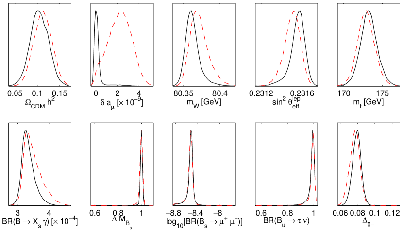
Results and analysis on neutralino dark matter and its direct detection prospects are presented in Section 5. A general feature of the results is that they exhibit some amount of prior dependence. This is clearly shown for the case of gluino-neutralino mass ratio in Subsection 4.5, the amount of fine-tuning in the parameters in Subsection 4.6, the muon anomalous magnetic moment (see the plots in Fig. 6), and the dominant neutralino dark matter annihilation/co-annihilation channels addressed in in Section 5. It is expected that with more precise and direct data from the Tevatron and/or the LHC would lift the prior dependence. However interestingly enough, some of the results, such as the mass of the lightest CP-even Higgs boson mass, are very similar for the different priors considered.
4.1 Parameters and sparticle mass posterior PDFs
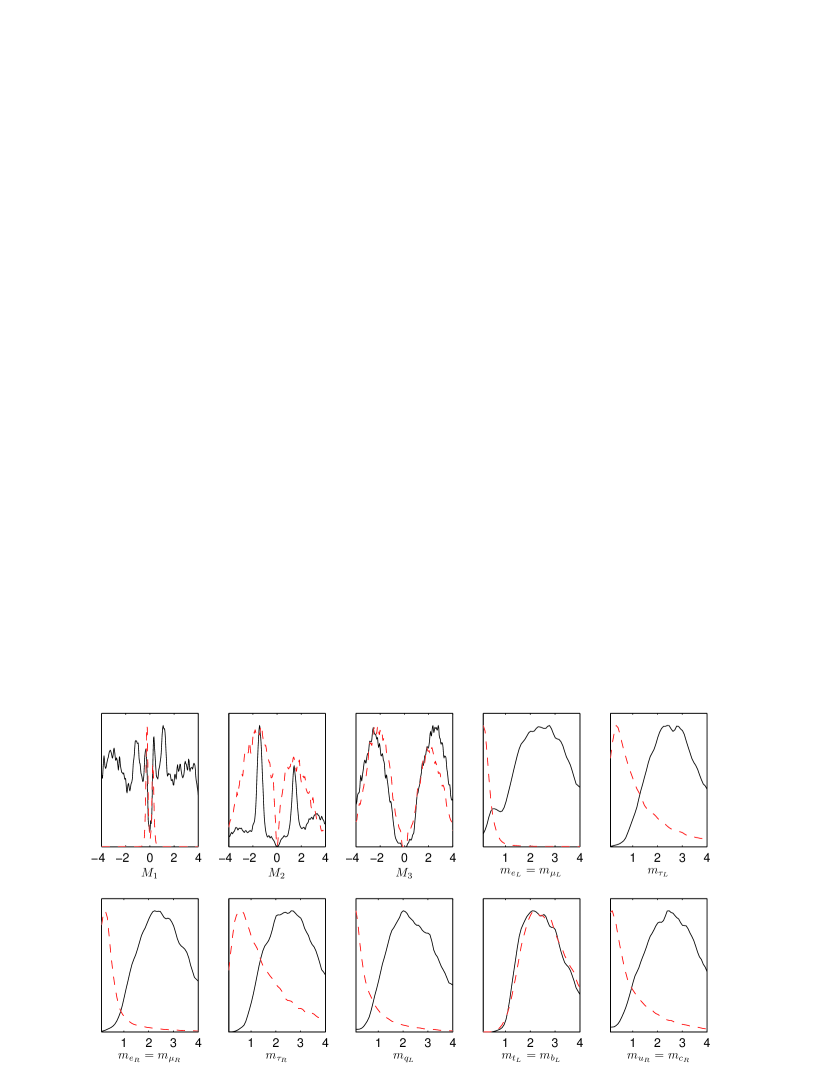
Our assumptions about the pMSSM priors are presented in Section 3.1. The priors are updated using the set of different experimental measurements explained in Section 3.2 via Bayes’ theorem (see Section 2.1). A measure of the amount of information in the likelihood can be seen from the results of the sampling procedure in the form of posterior PDFs. One dimensional marginalised posterior PDFs of the parameters are shown in Fig. 2.
 |
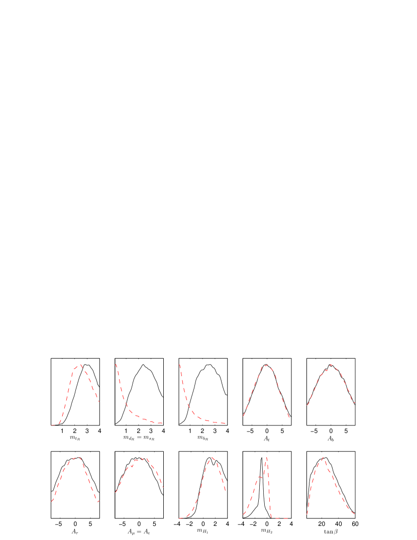 |
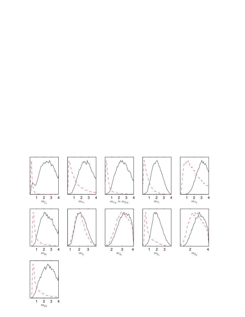
Most of the scalar mass terms in the log prior scenario are much reduced with respect to the corresponding mass term in the linear prior scenario, as expected. Changes to the scalar mass priors (in the log prior case) do change the posterior PDFs of and . This is because the dark matter likelihood is driving the fit, and dark matter co-annihilation requires the mass of the lightest neutralino (controlled by the smaller of and ) to be close to that of the scalar that it is co-annihilating with (see Subsection 5.2 for discussion on the co-annihilations in the pMSSM). On the other hand, shows approximate prior independence. For linear priors, upper bounds on the parameters come only from our constraint upon the prior range, there not being sufficient power in the data yet to constrain the parameters from becoming very large. , and have PDFs that tend to zero as the parameter tends to zero, but a finite bin-size means that this may not be evident in plots. Since and may take negative values, no logarithm was applied to them in the log priors case. Thus the apparent prior independence of is no surprise. The terms show a peak structure because if their magnitudes are too large, the squark mass becomes tachyonic and thus disallowed. Radiative corrections to the lightest CP-even higgs mass involving the stops imply that they must be quite heavy, above TeV in order to push the higgs mass above its direct search bound. Thus, the log prior only disfavours points at TeV by a factor of 1/2 compared to the lower values. In contrast, other sfermion masses which may be as low as 200 GeV obtain a log prior suppression of 1/20 at 4 TeV masses, i.e. the difference between log and linear priors is much more evident in that case. Thus there is no large enhancement of the posterior for small , which shows approximately identical posterior PDFs for the two different prior choices.
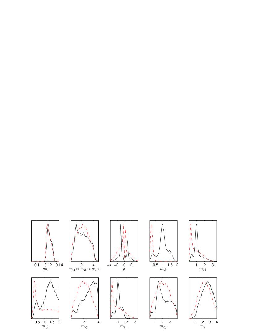
We display the posterior PDFs of the pole sparticle masses in Fig. 3 along with the posterior PDF of the parameter; and the 68 and 95 Bayesian credibility ranges for the sparticle masses in Tab. 5. The mass distributions can be understood from the parameters PDFs discussed above, since there is a rough one to one correspondence between the tree-level mass and a mass parameter for many of the sparticles. For the third family sparticles, the -terms and parameter contribute via the large mixing, which is proportional to the analogous SM fermion mass. The first and second generation sfermion masses are approximately degenerate, since the degeneracy is only broken by terms of order the second generation fermion mass, negligible compared to the sfermion masses. We see approximate prior independence of , , , and . Other sfermion masses show the expected log prior suppression at high masses.
 |
 |
| pMSSM fit (linear) | pMSSM fit (log) | |||
| Mass [TeV] | % interval | % interval | % interval | % interval |
The MSSM lightest CP-even higgs mass at tree level is,
| (51) |
but it receives large radiative corrections from third generation particles, of order 30 of its mass. Since the posterior is similar for both priors, then the tree-level value of will also be similar. An additional small prior dependence comes mainly from and prior dependence, but really the model itself constrains the higgs masses to be largely prior independent. The approximate mass degeneracy in the heavy Higgs masses and little dependence on priors can be seen to originate from the relationships between them. The tree-level MSSM pseudo-scalar CP odd higgs mass is given by
| (52) |
and it receives quite large radiative corrections. There is only a small prior dependence of , and Eq. 52 shows that the approximate prior independence of is something of an accident since and show some prior dependence, but this largely cancels in its effect on . Notice that
| (53) |
and since is usually far greater than and then holds, although loop corrections contribute to a small non-degeneracy, which however is not visible to the eye.
4.2 Good-fit points
For a given prior, the point with the highest likelihood is termed the best-fit point. We estimate a ‘good-fit point’ by picking the point with the highest likelihood out of the many millions sampled by the MultiNest algorithm. We shall see below that our under constrained fits exhibit parameter degeneracies, and so we should not expect the particular values of the good-fit parameters to be unique. Monte Carlo sampling methods are also ill suited to finding best-fit points, which are much better determined by hill climbing algorithms, for example. On the other hand, the properties of such a point are instructive to view in order to get a feel for which observables are pulling in which direction. The values of the parameters at the good-fit points are given in Tab. 6. The good-fit point of the linear prior has quite large SUSY breaking mass parameters, of the order of a couple of TeV in most cases, and large . On the other hand, the log prior sampling found a good-fit point with a mixture of sub-TeV and several TeV masses, because it spent more time exploring points with lower sfermion masses. It also has a moderate value of . Interestingly, both good-fit points have a negative parameter. This is in contrast to the CMSSM case, where the anomalous magnetic moment of the muon prefers positive . We shall discuss the sign of further in Subsection 4.4 below.
| Parameter | Description | Linear prior fit | Log prior fit |
|---|---|---|---|
| Bino mass | -2947 | -250 | |
| Wino mass | -1297 | -3017 | |
| Gluino mass | -2397 | -642 | |
| 1st/2nd gen. slepton | 1040 | 174 | |
| 3rd gen. slepton | 2640 | 993 | |
| 1st/2nd gen. slepton | 2301 | 201 | |
| 3rd gen. slepton | 3748 | 3530 | |
| 1st/2nd gen. squark | 878 | 165 | |
| 3rd gen. squark | 2301 | 2321 | |
| 1st/2nd gen. squark | 3027 | 1515 | |
| 3rd gen. squark | 2618 | 2905 | |
| 1st/2nd gen. squark | 1368 | 329 | |
| 3rd gen. squark | 1054 | 1268 | |
| top quark trilinear | -1963 | 651 | |
| b-quark trilinear | -3541 | 5727 | |
| -quark trilinear | 4725 | 3196 | |
| -quark trilinear | 2154 | 2951 | |
| down-type Higgs doublet | 2548 | 3445 | |
| up-type Higgs doublet | 882 | 669 | |
| Higgs vevs ratio | 52.0 | 21.0 | |
| top quark mass | 173.4 | 175.3 | |
| Z-boson mass | 91.186 | 91.190 | |
| b-quark mass | 4.16 | 4.26 | |
| 1/ | e-coupling constant | 127.95 | 127.91 |
| s-coupling constant | 0.1168 | 0.1161 | |
| higgs parameter | -942 | -770 |
We see the resulting MSSM spectra in Tab. 7, where the log prior good-fit point has some light sleptons and squarks. For the linear prior, all of the sparticles have masses around the TeV scale or higher.
|
![[Uncaptioned image]](/html/0904.2548/assets/x6.png) ![[Uncaptioned image]](/html/0904.2548/assets/x7.png)
|
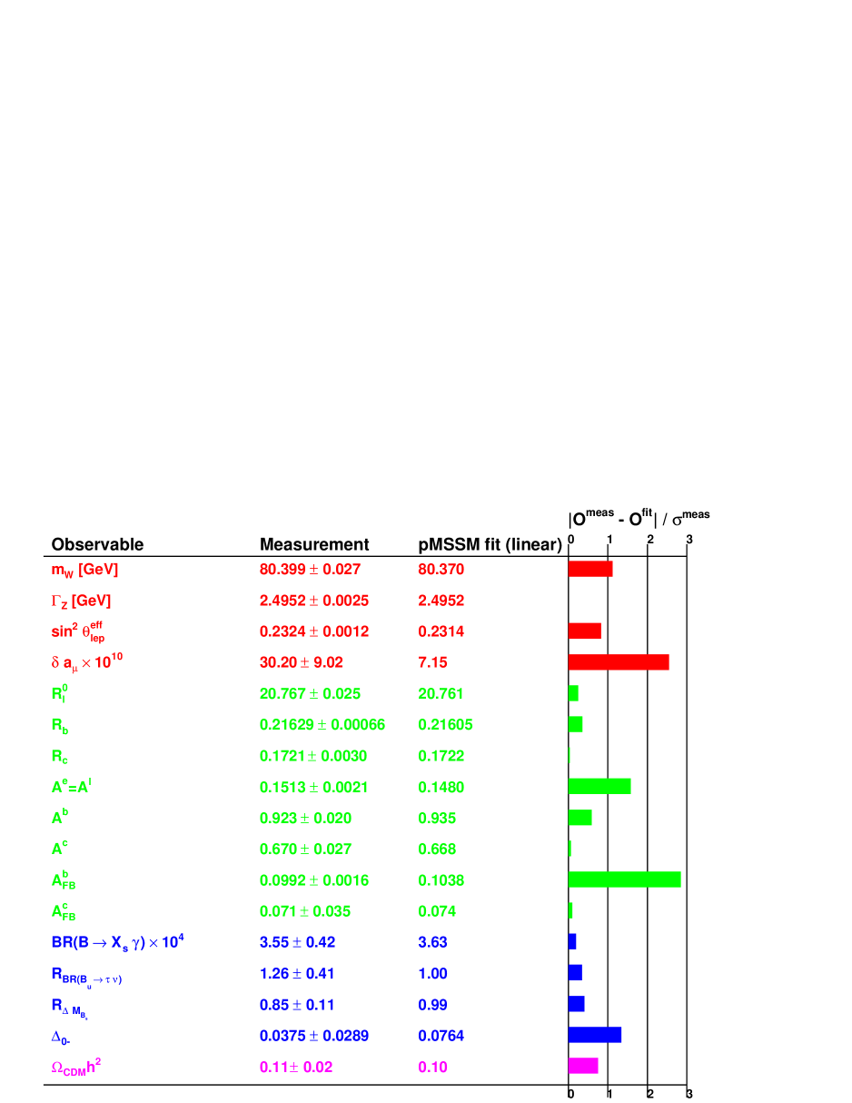
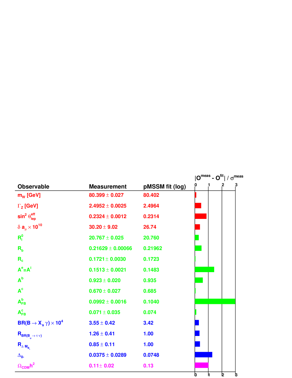
The statistical pulls of the various observables are shown in Figs. 4 and 5. We see that the observable that most discriminates between our two good-fit points is the anomalous magnetic moment of the muon, which is much better fit for the log prior point, where it receives large corrections from lighter slepton and gaugino masses. and also show a large difference between the two points, whereas most of the other observables display only a small difference in statistical pull between these two points. In fact, the log prior good-fit point has a significantly lower value (and therefore, a better likelihood). Were nested sampling perfect for finding the good fit point, the likelihood (or equivalently, the total ) values would be the same for both priors. This difference is therefore due to the finite sampling resolution of the posterior distributions.
4.3 Observables’ PDFs
The posterior PDFs for the observables used to constrain the pMSSM are given in Fig. 6. Differences between the two prior cases are mostly due to the fact that the sparticle mass PDFs are larger in the linear prior, leading to a suppression of SUSY effects in the loops of most observables. The -physics observables tend to have similar posterior PDFs in the two prior cases. In most of the EWPO, there are larger differences in the posteriors. For , there is a particularly large difference between the central values of the linear and log prior PDFs. The leading one-loop gaugino contribution at large is given by [96]
| (54) |
where and are positive loop functions proportional to for the case of degenerate sparticles in the loops. The dominant contributions coming from gauginos and sleptons therefore lead to an enhanced value of when they are lighter, as is evident for the log prior fits.
 |
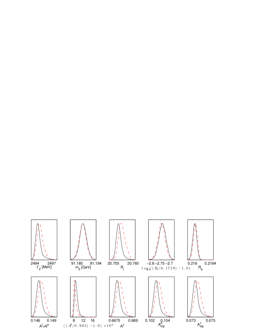 |
As we shall see in Section 5.2 and Tab. 10, the linear prior fits prefer Higgsino exchange to be the dominant LSP annihilation process, as opposed to slepton co-annihilation in the log prior case. This occurs at heavier neutralino LSP masses, and hence heavier smuon masses (which are always constrained to be heavier than the neutralino LSP). is then relatively badly fit as can be seen in the good fit point example where the statistical pull is more than .
4.4 Sign() comparison
The posterior PDFs in Fig. 3 indicates that the pMSSM prefers compared to . This is interesting since in the previous studies of CMSSM was seen to be preferred by the combination of and . One of the statistical tests (a predictive likelihood ratio test) in Ref. [41] found that the two measurements are incompatible in the CMSSM, but the other found no strong evidence for this and so the final conclusion of the analysis remains unclear. The sign of the SUSY contribution to is dependent upon the sign of . There are two dominant SUSY contributions to consider: the first comes from diagrams involving a charged Higgs boson and up-type quarks. The second, involving a chargino and up-type squarks, depends upon the sign of the product . Eq. 34 indicates that there is a preference for a positive total contribution at the 1- level. In the CMSSM, is typically negative due to RGE effects. Eq. 54 shows that the sign of the non-SM contribution to the muon anomalous magnetic moment depends upon the sign of and . In the CMSSM, and are positive and so the combination of the and constraints implies a preference for a definite sign of . Bayesian analyses [13, 34] demonstrated that the current statistical evidence for in the CMSSM is weaker than many may pre-suppose.
We have not used the freedom to re-define the phases of the fields and make positive for example, and so negative appears in our fits. As such, in the pMSSM both and , may take either sign and so the preference for is broken and we may expect that the dominant contributions to the observables do not prefer either sign. On the other hand, there may be some residual dependence from the sub-dominant contributions, as well as sub-dominant radiative corrections to other observables. Thus it is still important to check the relative probabilities for . For the pMSSM with a linear prior measure we find the following probability for the two signs of :
| (55) |
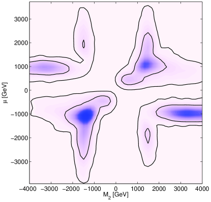
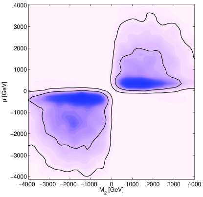
Fig. 7 shows the posterior PDF marginalised on the plane. The figure shows that, although opposite signs for are allowed, it is constrained to have the same sign as , especially for log priors where is well fit. For linear priors, the large volume of parameter space leading to heavy sparticle masses mean that this tendency is reduced and there is a small amount of probability that , predicting a small negative . Fig. 7 clearly shows a symmetry of the fits when one simultaneously flips the signs of and , as should be the case due to phase re-definition freedom.
 |
 |
The SM prediction of remains somewhat controversial. The hadronic contributions that are extracted from and data disagree, and one obtains quite different constraints depending upon which data set is used. To quantify the extent to which our mild preference for depends on the observable, we made a separate sampling with all except the constraints. We found that is still more probable with:
| (56) |
Thus, contributes around 0.06 to the probability of , the other observables including contributing around 0.04. However, computing the Bayesian evidence ratios in the two scenarios indicate that there are no conclusive evidence, based on Jeffrey’s scale (see Tab. 1), for one particular sign() over the other. The odds and logarithm of the evidence ratios are summarised in Tab. 8.
| Data Considered | Odds, | Remark | |
|---|---|---|---|
| All constraints | Inconclusive | ||
| All minus constraints | Inconclusive |
4.5 The gaugino code
The LHC being a proton-proton scattering machine, is going to be producing a large number of strongly interacting particles. If TeV-scale SUSY is nature’s choice of physics then the LHC machine would eventually be a gluino factory. The gluinos would cascade-decay down to the neutralino LSP. Thus the visible energy of the decay products of the gluino is determined by the gluino-LSP mass splitting. If the ratio of these two masses is large, there will be high visible energy and it should be easier to pick SUSY out from underneath backgrounds. The nature of the gluino and neutralino sparticles could also be important in discriminating the different models of SUSY. As recently emphasised [110], patterns of gaugino masses can be used as an early discriminant of models of SUSY breaking at the LHC. The argument for this goes as follows. In, for instance, the CMSSM or minimal gauge-mediated SUSY-breaking, the boundary conditions of the values of the gauge coupling constants take the form around the TeV scale. Here , or respectively represent the electromagnetic, weak or strong interactions couplings. Unification of the gauge couplings at a GUT scale, gives a prediction on the pattern of gaugino mass terms since the ratio does not run at one loop [111]. If the neutralino is gaugino dominated, this translates into some gluino-to-neutralino mass ratio pattern.
Already there are distinct ratios coming from viable SUSY breaking scenarios. For instance, the CMSSM (and AMSB) if it has a predominantly bino (and wino) LSP predicts (and 9, respectively) [110]. Mirage mediation [112] with predominantly bino LSP and the large volume scenario (LVS [113, 114, 115, 116]) have a characteristic ratio less than 6 and between 3 to 4, respectively (with the LVS having the most compact gaugino mass pattern). Higgsino components of the neutralino LSP spoil a strict prediction of the mass ratio coming from gaugino mass ratios, however. By construction, the pMSSM set-up is the most generic and natural approach for MSSM phenomenology. We show the pMSSM posterior PDF for the gluino-to-neutralino mass ratio in Fig. 8 which provides a clear discrimination between the pMSSM and the other models. The figure 8 shows a sharp dependence of the gluino-to-neutralino mass ratio posterior PDF on the choice of prior. The linear prior predicts a compact gaugino mass ratio with888See [32] for similar results from a pMSSM analysis done with a different set of observables than in this work. . For the log prior case a much broader distribution of mass ratios centred around results from the fits.
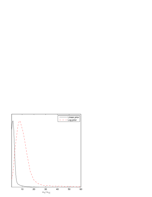
It is worthwhile to point out the source of the difference between the peak positions in Fig. 8. The gluino mass, , PDF is roughly the same for both priors. This implies that the numerator is fixed with respect to the two different priors. So the shift is solely due to the different properties of which is much lighter for the log prior choice.
4.6 Fine-tuning
The main motivation of weak-scale SUSY is to solve the technical hierarchy problem, explaining why the Higgs boson remains at the weak scale despite quantum corrections which are as large as the largest mass scale in the theory (e.g. the Planck scale). In order for softly broken SUSY to still provide a resolution of the technical hierarchy problem, the SUSY breaking terms should not be much larger than the TeV scale, otherwise an a priori un-natural cancellations between radiative corrections are required in order to keep the Higgs boson mass low. Direct SUSY search limits imply lower bounds on sparticle masses, which already start to imply that the MSSM parameters must cancel somewhat in order to separate the electroweak and SUSY breaking scales. This is termed the ‘little hierarchy problem’ [117, 118], (see a recent discussion in [119]). We wish to quantify the necessary amount of fine-tuning in the pMSSM parameters needed to make the set-up consistent with the imposed sparticle mass bounds.
We follow the approach in [120], quantifying the amount of fine-tuning in the Z-boson mass prediction coming from Higgs potential minimisation conditions. We consider this as a measure of fine-tuning in the pMSSM. The tree-level Z-boson mass is given by
| (57) |
where
| (58) |
The amount of fine-tuning is quantified by considering the sensitivity of to a variation of a parameter [121]:
| (59) |
where and are the relevant parameters in the pMSSM. Assuming , from Eqs. 57, 58 and 59, one derives:
| (60) |
, , and are added in quadrature to obtain an over-all measure of fine-tuning, :
| (61) |
Values of far greater than unity indicate large fine-tuning.
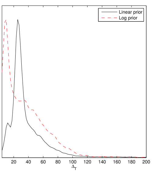
The posterior PDF for the amount of fine-tuning in the pMSSM is shown in Fig. 9. The logarithmic prior scenario have lower than in the linear prior. This is not surprising since the SUSY breaking terms are much reduced in the former scenarios than in the latter. We see from the figure that the fine-tuning is most likely low at around , but there is a tail extending beyond . One could use a prior of , to encode a belief in less fine-tuned points in our global fits [11]. Alternatively, one could place a cut on , but the value of such a cut is of course subjective. 82 of the high posterior PDF points, around of samples, have , so a hard cut placed at 10 would have a drastic effect on the fits. Here we decline to change the prior or place cuts, since we are content with observing that, for most of the probability mass in the fits, it is not unacceptably large. For the highest likelihood models the fine-tuning is reduced from its average. For example, for the good-fit point in the linear prior sample, , whereas for the good-fit point in the log prior sample, .
Notice that in general the amount of fine-tuning we find is small compared to previous studies of the MSSM that start at a high scale, running down to the TeV scale using the RG equations. The reasons for this include, as explained in Refs. [122, 118], that the amount of fine-tuning is a function of the cut-off scale and tends to decrease with this scale because the interval of RG running of the soft parameters induces EWSB at tree level and the cross-talk (through RG running) between parameters in the Higgs sector and those from the squarks, gluinos, etc sectors is drastically reduced such that the latter parameters can be much heavier than without disturbing the naturalness of the electroweak scale999We thank J. R. Espinosa for interesting conversations on this point and on fine-tuning in general.. Ref. [122] found some approximate semi-numerical solutions of the RGEs for the case that the boundary conditions on SUSY breaking parameters are set at the GUT scale GeV. The dominant term in typically comes from cross-talk with the GUT scale gluino mass :
| (62) |
where the authors determined the coefficient numerically: and , for example. This is to be contrasted with the pMSSM in Eq. 60, where the terms in are set at the SUSY breaking scale and are , and do not involve the gluino mass, upon which there are strong empirical lower bounds.
5 Neutralino Dark Matter
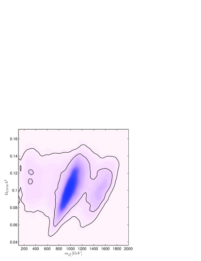
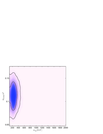
Assuming R-parity conservation the lightest supersymmetric particle (LSP) may be a good dark matter (DM) candidate. In Ref. [25], a pMSSM study of the ability of SUSY measurements at future colliders to constrain dark matter properties was considered. We assume that the neutralino LSP constitutes the DM in the universe. The DM relic density then depends upon the LSP mass and, through its composition in terms of gauginos and Higgsino, its interactions. 2-D marginalised posterior PDFs showing preferred regions in the relic density versus LSP mass are shown in Fig. 10. There is a mild positive correlation between the preferred mass and the dark matter relic density for linear priors which is not evident for the log priors. It is clear that the LSP mass is not well constrained by current data, since it is highly prior dependent. The nature of the neutralino LSP in the pMSSM is addressed in Section 5.1. The mass difference between the LSP and the next to lightest supersymmetric particle (NLSP) is important because if it is small, the LSP may efficiently co-annihilate, in the early universe, with the NLSP, significantly reducing the relic density. The different possible NLSPs in the pMSSM with the corresponding posterior probabilities are listed in Section 5.2. The dominant (co-)annihilation channels are presented in Section 5.2. We present the prospects of direct dark matter detection in Section 5.3.
 |
 |
5.1 Neutralino dark matter composition
The nature of the neutralino LSP determines the (dominant) processes by which it (co-)annihilates into SM particles and therefore affects its present number density. This was illustrated using the randomly scanned pMSSM samples in [4] where it was shown that the nature of the neutralino LSP depends upon whether one assumes that the LSP makes up all or only some of the DM relic density. The neutralino mass matrix is given by where and,
| (63) |
and . The neutralino mass eigenstates are where N is a unitary transformation that diagonalises . The LSP neutralino mass eigenstate is therefore a mixture of bino, wino and Higgsino:
| (64) |
Different regions of parameter space give different neutralino LSP compositions. When , and the LSP is dominantly bino. Bino LSPs give a relic density that is too high for most of the parameter space unless some specific mechanism (such as efficient co-annihilations or annihilations through a resonance) is working. When , dominates, i.e. the LSP is dominantly wino and is quasi mass degenerate with the lightest chargino. This leads to strong co-annihilations between the LSP and the chargino, and typically the relic density much smaller than the WMAP constraint for wino LSPs. For , and are of order one and the LSP is dominantly Higgsino and there may be efficient annihilations into top and weak gauge boson pairs. In the Higgsino-dominated LSP scenario, , , are almost all mass degenerate and are Higgsino-like. Of course, there exist mixed cases which include several of these limiting behaviours.
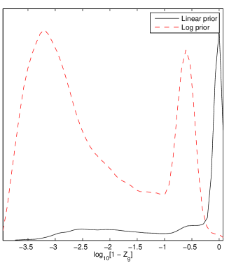
The gaugino/Higgsino mixture PDF of the LSP is shown in Fig. 11 constructed from the fraction
following [123]. is unity if the neutralino LSP is fully Higgsino-like and zero if fully gaugino-like. The plot shows that LSP is mostly Higgsino in the linear prior case, similar to the non-universal higgs mass scenario [124], and mostly gaugino for the log prior scenario. Thus, current data do not unambiguously constrain the LSP content. Referring to Tab. 6, we see that the good-fit point from the linear prior sample has a mixed wino-Higgsino LSP (more precisely, the point has and ). The log prior sample good-fit point has a bino dominated LSP (), but there are several light sparticles, allowing sufficient annihilation.
5.2 (Co-)Annihilations
At early times of the universe the LSP is in thermal equilibrium with other particles and, ignoring for now co-annihilations, its number density evolution is governed by the Boltzmann equation
| (65) |
Here is the Hubble expansion rate of the universe, is the number density and is the thermally averaged annihilation cross sections of the neutralino LSP. is the relative velocity of the annihilating pair. The LSP annihilation rate is given by . At a freeze-out temperature , the neutralino decouples, . Substituting into Eq. 65 predicts that the LSP relic density is inversely proportional to the thermally averaged annihilation cross section, . This means that for the LSP relic abundance today to be in the WMAP-5 range Eq. 47 there must be a significant number of annihilations of the neutralino LSP at earlier times. The possible processes are mostly two-particle final states which could be fermion anti-fermion pair, combinations of the weak gauge-bosons or combinations of the Higgs bosons (see e.g. [125]). The discussion becomes much more involved once co-annihilation processes are taken into account, since coupled Boltzmann equations are required for each relevant SUSY particle species.
Co-annihilation processes dominate in parameter space points where next-to-lightest supersymmetric particle (NLSP) that are almost mass degenerate with the LSP. At such points the neutralino abundance also depends strongly on the annihilations of the NLSPs [126, 127] and the number densities of the LSPs and NLSPs are coupled. A review of different co-annihilation studies was presented in [4]. Here we present and analyse the outcome of the pMSSM annihilation and co-annihilation results for our two different prior measures. We shall only discuss processes that contribute 1 or more of the annihilation cross section.
In Tab. 9 we give a list of possible NLSPs and corresponding posterior probabilities for each. The probabilities indicates that neutralino-chargino co-annihilations are most likely to be dominant in the pMSSM with a linear prior measure. For the log prior measure, neutralino-slepton co-annihilations are the most probable. We illustrate the abundance and complexity of the annihilation channels by presenting the dominant ones at the good fit points in Tab. 10. The dominant channels for the linear prior sample good-fit point are direct neutralino-chargino co-annihilation and neutralino annihilation via chargino exchange into - and -boson pairs. For the log prior measure good-fit point, the dominating channels are neutralino co-annihilations with various sleptons. Many different processes contribute at the percent level. We present the identities of the dominant channel, along with its posterior probability in Tab. 11. The most likely channel is neutralino-chargino co-annihilation for the linear prior and neutralino annihilation for the log prior. From the large prior dependence in the results, we deduce that current data are not sufficient to constrain the dark matter annihilation properties of the LSP.
| NLSP | ||
|---|---|---|
| 14% | 1% | |
| 77% | 15% | |
| 1% | 0% | |
| 2% | 39% | |
| 0% | 4% | |
| 0% | 2% | |
| 0% | 27% | |
| 0% | 7% | |
| 1% | 1% | |
| 1% | 1% | |
| 1% | 1% | |
| 1% | 0% | |
| 1% | 1% |
| Linear Prior | Log Prior | ||||||
|---|---|---|---|---|---|---|---|
| Event | Event | Event | Event | ||||
| 3 | 2 | 2 | 2 | ||||
| 3 | 5 | 4 | 14 | ||||
| 10 | 10 | 4 | 14 | ||||
| 3 | 3 | 2 | 3 | ||||
| 3 | 2 | 2 | 3 | ||||
| 2 | 1 | 9 | 1 | ||||
| 1 | 1 | 2 | 9 | ||||
| 1 | 2 | 1 | 1 | ||||
| 1 | 2 | 9 | 1 | ||||
| 3 | 3 | 2 | 1 | ||||
| 2 | 1 | 1 | 1 | ||||
| 1 | 1 | 1 | 1 | ||||
| 3 | 1 | 1 | - | - | |||
| 1 | 2 | - | - | - | - | ||
| 4 | 4 | - | - | - | - | ||
| 1 | 1 | - | - | - | - | ||
| 1 | 1 | - | - | - | - | ||
| (Co-)annihilation | Linear prior case | Log prior case |
|---|---|---|
| 35% | 5% | |
| 20% | 28% | |
| 0% | 7% | |
| sleptons | 0% | 23% |
5.3 Direct detection
Many different experiments search for the nature of dark matter (e.g. see [128] and references therein). Indirect detection experiments are designed to observe the annihilation products of dark matter particles. We do not address indirect detection here and save it for future consideration. Here, we consider direct detection experiments such as XENON [129], CDMS [130, 131], ZEPLIN [132, 133], Edelweiss [134], CRESST [135], WARP [136, 137] or COUPP [138]. Such experiments are designed to observe the elastic scattering of dark matter particles with nuclei. The LSP may interact with quarks in target nuclei via -channel CP-even Higgs exchange or -channel squark exchange and with gluons via squark loop contributions. DM direct detection rates also depend on the local neighbourhood DM density and velocity distribution. The density, which is estimated to lie between and ( GeV/), is inferred by fitting observations to models of galactic halo [139, 140]. The velocity is expected to be around km/s [141].
The elastic scattering cross section is partitioned into spin-dependent and spin-independent components. The spin independent part is currently the most constraining, and we concentrate on it. It is proportional to the square of the target nucleus atomic number, . This enhancement is because the dark matter wavelength is of same order as the size of a nucleus and hence the scattering amplitudes on individual nucleons add coherently. There is one experimental claim in direct detection experiments of a signal in the annual modulation rate [142]. This result has not been confirmed by other experiments and would be incompatible with a neutralino LSP candidate, so we do not use it to constrain the pMSSM. Aside from this, no positive signal has been detected to date in dark matter detection experiments. A positive signal would constrain SUSY parameter space if one assumed a particular local neighbourhood DM density and velocity distribution.
The spin-independent neutralino-nucleus elastic scattering cross section is given by
| (66) |
where is the mass of the target nucleus and and are the atomic number and atomic mass of the nucleus, respectively. and are the neutralino’s couplings to protons and neutrons, given by [143]
| (67) |
where are the neutralino-quark couplings [143, 144, 145, 146, 147, 148] and denote the quark content of the nucleon. They have been experimentally bounded to be: , , , , and [149, 150, 151]. The first term in Eq. 67 corresponds to interactions with the quarks in the target, which can occur through either -channel CP-even Higgs exchange, or -channel squark exchange. The second term corresponds to interactions with gluons in the target through a quark/squark loop. is given by , and analogously, .
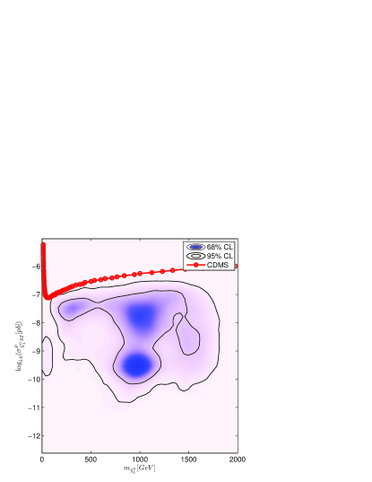
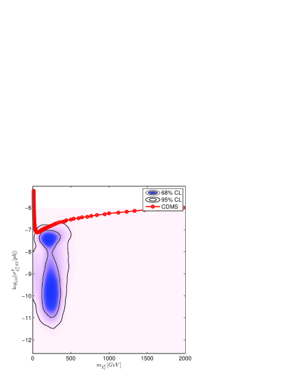
|
The direct detection constraints from the cryogenic cold dark matter search (CDMS) experiments on the pMSSM is shown in Fig. 12. The large prior dependence of the results indicates that current data are insufficient to constrain the direct detection cross sections. One can say that there is clearly a wide allowed range for the direct detection cross sections.
5.4 Relaxing the purely LSP dark matter assumption
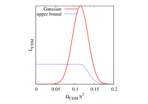
The analysis presented above was done assuming that the neutralino LSP is the only source of dark matter. It is known that the LSP relic density is sensitive to the assumed cosmology. For example, Big Bang Nucleosynthesis (BBN) expansion rates can enhance the calculated relic density without affecting other important cosmological quantities [152]. The inclusion of right-handed neutrinos could change the relic density prediction, see for instance [153]. One could also allow for additional non-neutralino dark matter components. In order to see the potential effect of such model changes, we relax the constraint from the DM relic density to the case where only predictions larger than the central values are penalised according to the likelihoods:
| (68) |
where is the experimental central value quoted above and is an inflated error on relic density that includes theoretical uncertainties in its prediction.
We have made an independent run using Eq. 68, i.e. relaxing the purely LSP DM assumption, i.e. implicitly assuming some other component of dark matter. We wish to examine the amount of DM that comes from the LSP. These runs were performed in Ref. [32], where the relevant constraints can be found. Linear priors were used on the parameters, which had a 2 TeV upper bound. We find in Fig. 14 that the preferred relic density is low compared with the purely LSP DM assumption: around . Thus once one allows for an additional component of DM to the LSP, the model prefers the additional component to dominate the relic density 101010Some of us hope to return to this issue in future work. We thank Bryan Webber for suggesting this comparison..
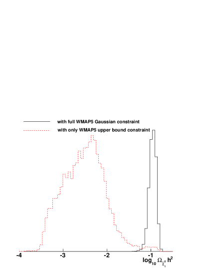
6 Conclusions and Outlook
We have presented the first statistically convergent global fit of the pMSSM model with its 25 independent continuous parameters plus a discrete parameter, , to the dark matter relic density, indirect observables and direct sparticle search constraints. We have used the entire set of relevant electroweak precision observables and -physics data, as well as the anomalous magnetic moment of the muon as indirect observables. The evidence for the linear and log prior measure pMSSM in light of the data is and respectively. We have presented a good-fit point in the pMSSM parameter-space which is not unique since the minimum is degenerate. All the different parameter-space points with maximal likelihood are equally interesting for phenomenological studies.
This work constitutes a technical demonstration that statistically convergent global fits in high dimensions involving curving degeneracies and several modes are now feasible. This feasibility is due to new sampling algorithms and improvements in the speed of computation and access to it. It allows more complete phenomenological studies of multi-parameter models beyond the standard model that could not have been completed in the past. In particular, the set-up and techniques employed here provide an unbiased approach to MSSM phenomenology – independent of the underlying theory, the mechanism to break SUSY or its mediation – hence it could lead to more robust SUSY phenomenological studies and guides for LHC SUSY searches and for dark matter search experiments. As expected the results of this exercise differs significantly from those of the more studied CMSSM/mSUGRA and thus the pMSSM parameter space provides a much richer and appropriate arena for LHC studies of the MSSM.
For the analysis we consider prior measures flat in either the parameters (a linear prior) or flat in the logarithm of the parameters (a log prior) in order to check robustness of inferences. Given the large number of (the pMSSM) parameters compared with the (weak constraining power of the) data available at the moment it is very interesting that indeed there are some prior-independent results or inferences. The lightest CP-even Higgs boson mass and the stop masses fall into this category of robust and prior independent results. The other sparticle masses and all dark matter properties exhibit significant prior dependence and require more direct and precise data (or more constrained models) to make their prediction robust. We emphasise that prior dependence is present and it is a positive feature of Bayesian methods, since its absence signals when there is enough data to make the fits robust. This can be used as a guideline for future studies of the experimental implications of the MSSM. In particular, if SUSY is discovered via sparticle production at collider and many sparticle properties are precisely measured, it will be possible to use the techniques show-cased in the present work to extract pMSSM information. Such information can then be checked for consistency with more constrained models.
We now contrast our methods with the recent random points scan analysis of the pMSSM in Ref. [33] and a similar earlier work in Ref. [4]. These works perform a pMSSM random parameter scan to find points which pass direct search and dark matter constraints while being within 2 of the central values of some indirect constraints. All such points are considered on an equal footing, and as such (as emphasised by the authors) are not a statistical global fit. We, on the other hand, allow a trade-off between different observables in a statistically correct fashion; one may tolerate a moderately bad fit in one observable if it fits the other observables particularly well. Our use of Gaussian distributions for the likelihoods (instead of the 2 top-hat function in [4, 33]) is justified by the central limit theorem and the maximum entropy principle [154]. Interesting points with LHC phenomenology not covered by previous studies of constrained models were found in Ref. [33], which was the main aim of the approach (a few thousand points passed the constraints, out of scanned). We aim to perform a complete and statistically convergent global fit of the pMSSM. To achieve this we take advantage of the power of the MultiNest algorithm, which provides samples in moderately high dimensional parameter spaces (with curving degeneracies and different modes) much more efficiently than in random/grid parameter scans. In [33] there was more emphasis on direct search limits, which are more sophisticated than the ones employed in the present paper. Since the sparticle masses implied by our fits are large, our results are insensitive to the exact form of the direct search limits. The density of points in Ref. [33] also shows prior dependence although the results were not interpreted statistically (and thus they were not Bayesian nor frequentist). Another major difference to our approach is that in Ref. [33], the WMAP constraint is used only as an upper bound (making viable points much easier to find) and so the existence of another non-MSSM dark matter particle is assumed. This changes the character of the points: allowing MSSM points which predict approximately zero LSP relic density means that a large number of sampled points have a wino dominated LSP. We, however, assume in most of our analysis that the neutralino constitutes all of the dark matter. In Section (5.4) we presented an independent run made using the WMAP constraint only as a lower bound and our results (as expected) agree with those of [4, 33] in the sense that, in that case, the LSP contribution tends to be only a small fraction of the total dark matter.
There are many directions in which this research could be extended. For each of the tens of thousands of preferred points in our sample, a detailed calculation of LHC observables such as inclusive counts of opposite sign dilepton and trilepton events, could be made using standard event generators and detector simulators, as has been done for more constrained models such as the CMSSM [155]. This would provide a portrait of the signature space that may eventually be useful in direct SUSY searches. On a simpler level, one could compute relative probabilities of various sparticle mass hierarchies. The indirect dark matter detection prospects could also be evaluated, although with current data, they are likely to be highly prior dependent. The impact of the inclusion of the fine-tuning into the prior could be analysed. Assuming a particular parameter point, the impact of LHC SUSY measurements on our fits could be evaluated and an estimate of how much luminosity would be required in order to make inferences approximately prior independent111111A Bayesian approach has recently been used to ameliorate the LHC inverse problem in the MSSM by combining LHC data with indirect observables [156].. In this case, model comparison between more constrained models and the pMSSM could be informative. One could determine, for a given LHC luminosity, which models could be made prior independent. The extension of the analysis to the full 124 MSSM parameter space may be still out of reach at the moment. Algorithms improving the MultiNest algorithm may be required before attempting it. Adding a small number of minimal flavor violating parameters could however be feasible. An extension of this work to include reasonable generalisations of the minimal flavour violation scenario adding a few extra parameters should be possible. Also, including R-parity violation to the pMSSM as well as a phenomenological NMSSM are within reach of the techniques we used here. Some of us hope to return to these issues in future work.
Appendix A Nested sampling and the MultiNest algorithm
For scanning parameter spaces of large dimensionality we have to use efficient modern approaches for sampling the posterior. In such problems, interesting parameter regions are often tiny in some directions and many directions are orthogonal to ones along which the likelihood is degenerately high. In this Section we present the procedure, in the context of the pMSSM, for the Monte Carlo technique called nested sampling developed by John Skilling [31] and implemented in MultiNest. It is a general method for evaluating the integral Eq. 2 from which representative samples from the posterior distribution Eq. 1 are obtained as by-product. The method differs from the traditional approach to inference dating back to Metropolis et. al. (1953) where the emphasis is more on evaluating the posterior density than in calculating the evidence. Skilling’s method goes as follows. Exploring the 25-dimensional co-ordinate to evaluate the evidence integral is impractical. Instead, the prior mass can be used directly to convert the 25-dimensional into a 1-dimensional integral over a unit interval. Let be the prior mass enclosed within the likelihood contour, in the parameter space. That is,
| (69) |
As increases from zero to infinity the enclosed prior mass decreases from to . The inverse function is the contour value (a likelihood value) such that the volume enclosed is (see Fig. 15 for an illustration). Eq. 69 and the definition of its inverse implies that the evidence Eq. 2 can be expressed as
| (70) |
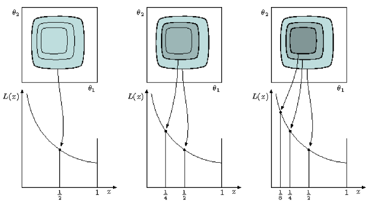
Given the likelihood values at a sequence of points the evidence is estimated as a weighted sum,
| (71) |
where for the trapezoidal rule .
A.1 Evidence evaluation
The nested sampling procedure for evaluating the evidence starts with the accumulation of points uniformly drawn from the prior, the initialisation of the evidence, , and the initialisation of the prior volume, . The number, , of “live” points, is preserved throughout the procedure and every point is associated with its corresponding likelihood value: . Each step over the iterations is associated with the lowest likelihood (or the largest prior mass, ) that defines the contour line (or shell) over parameter space. For moving from the th to the th iteration a new point is drawn from the set of points uniformly distributed in , the parameter space region with likelihoods . This is illustrated in Fig. 16. The new point replaces the one with lowest likelihood. is set to , the weight to and the evidence incremented by . This procedure is repeated for the subsequent iterations.
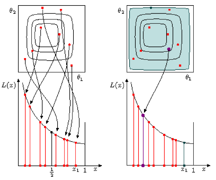
The prior volume shrinkage ratios are distributed according to in where is the largest of random numbers uniformly distributed in . Sampling over represents a geometrical exploration of the parameter space. The mean and standard deviation of are
| (72) |
respectively. This justifies the assignment since each draw of is independent and after iterations of the sampling procedure the prior volume will shrink down according to
| (73) |
A.2 Stopping criterion
The nested sampling procedure is terminated after a preset number of the iterations (as described in Subsection A.1) or when the largest likelihood taken over the whole currently (at the instance of check for termination, say the th iteration) available prior mass would not increase the evidence value by more than some preset fraction (we use 0.5 in log-evidence). That is, the procedure is terminated if
The integration, , is dominated around the region , wherever the bulk of the posterior mass is to be found. Here
| (74) |
and is the compression ratio representing the fraction of the prior mass that contains the bulk of the posterior. . Recalling that we expect the integration procedure to take steps (iterations) before reaching covering the bulk of the posterior. Hence another termination condition could be to continue iterating until the count is significantly greater than .
The uncertainty in translates to a geometrical uncertainty factor in the weights of the dominating iterates. This in turn gives the uncertainty in the evidence via Eq. 71 as so that
| (75) |
A.3 Posterior inferences
The posterior distribution is simply the prior distribution weighed by the likelihood. This can be trivially extracted from the evidence calculation since the set of sampled points is already a posterior representative provided it is assigned the appropriate importance weight and normalised by the evidence, , to produce probability density with unit total. That is at the th iteration the posterior probability density is
| (76) |
These are generated from the sequences of discarded points (the points with the lowest likelihood value at each iteration) during the sampling procedure. From these posterior sequence properties such as the mean and standard deviation of some are easily computable:
| (77) |
Equally-weighed samples selected proportionally to can be used to construct marginalised posterior distributions in .
For completeness, it is worth mentioning that there are alternative
methods for evaluating the evidence with other advanced MCMC
algorithms like thermodynamic integration and it is not
clear yet which method is best for high dimensional problems:
dimensions greater than 121212We thank David Mackay for
interesting discussions about
this. See for example
http://www.inference.phy.cam.ac.uk/mackay/presentations/nested06/ 10.
However, for this paper we implement the nested sampling algorithm for
our purpose using the MultiNest code [29] which has
additional quality of being efficient in sampling multi-modal
posteriors exhibiting curving degeneracies (see a summarised account
in Subsection A.4).
A.4 MultiNest
The most challenging task in implementing the nested sampling algorithm is drawing samples from the prior within the hard constraint at each iteration . Employing a naive approach that draws blindly from the prior would result in a steady decrease in the acceptance rate of new samples with decreasing prior volume (and increasing likelihood). MultiNest algorithm [29, 30] tackles this problem through an ellipsoidal rejection sampling scheme by enclosing the live point set into a set of (possibly overlapping) ellipsoids and a new point is then drawn uniformly from the region enclosed by these ellipsoids. The number of points in an individual ellipsoid and the total number of ellipsoids is decided by a an ‘expectation–maximisation’ algorithm so that the total sampling volume, which is equal to the sum of volumes of the ellipsoids, is minimised. This allows maximum flexibility and efficiency by breaking up a mode resembling a Gaussian into relatively fewer number of ellipsoids, and if the posterior mode possesses a pronounced curving degeneracy so that it more closely resembles a (multi–dimensional) ‘banana’ then it is broken into a relatively large number of small ‘overlapping’ ellipsoids (see Fig. 17). With enough live points, this approach allows the detection of all the modes simultaneously resulting in typically two orders of magnitude improvement in efficiency and accuracy over standard methods for inference problems in cosmology and particle physics phenomenology (see e.g.[157, 158, 34, 32, 159]). The MultiNest procedure as applied to our pMSSM fits is summarised by the flow charts in Fig. 18.


|
 |
Acknowledgments.
We would like to thank Arne Weber for help with fixes to the code SUSYPOPE, A. Pukhov for help with micrOMEGAs, N. Mahmoudi for her help with SuperIso, and M. Dolan for checks with the likelihood code. We thank S. Abel, J. Conlon, D. J. C. MacKay, J. R. Espinosa, S. Krippendorf, C. Lester, M. Gomez-Reino, F. Marchesano, P. Slavich, K. Suruliz, A. Uranga, B. Webber and E. Witten for useful discussions. The calculations performed in this paper were done using the Cambridge High Performance Computing Cluster (HPC) Darwin and COSMOS, the UK National Cosmology Supercomputer. We thank Andrey Kaliazin, Stuart Rankin and Victor Travieso for assistance in setting and running the codes on these computing facilities and John Turner and the HPC group for important assistance regarding the rights to use HPC. This research was partially funded by STFC. SSA is supported by The Gates Cambridge Trust and thank the African Institute for Mathematical Sciences (AIMS) for hospitality during the early stages of this work. FQ thanks the organisers of the Cooks Branch 2009 meeting for hospitality during the last stages of this work.References
- [1] D. J. H. Chung et. al., The soft supersymmetry-breaking Lagrangian: Theory and applications, Phys. Rept. 407 (2005) 1–203, [hep-ph/0312378].
- [2] R. L. Arnowitt and P. Nath, Cosmological constraints and SU(5) supergravity grand unification, Phys. Lett. B299 (1993) 58–63, [hep-ph/9302317].
- [3] J. R. Ellis, K. A. Olive, Y. Santoso, and V. C. Spanos, Likelihood analysis of the CMSSM parameter space, Phys. Rev. D69 (2004) 095004, [hep-ph/0310356].
- [4] S. Profumo and C. E. Yaguna, A statistical analysis of supersymmetric dark matter in the MSSM after WMAP, Phys. Rev. D70 (2004) 095004, [hep-ph/0407036].
- [5] E. A. Baltz and P. Gondolo, Markov chain Monte Carlo exploration of minimal supergravity with implications for dark matter, JHEP 10 (2004) 052, [hep-ph/0407039].
- [6] J. R. Ellis, S. Heinemeyer, K. A. Olive, and G. Weiglein, Indirect sensitivities to the scale of supersymmetry, JHEP 02 (2005) 013, [hep-ph/0411216].
- [7] L. S. Stark, P. Hafliger, A. Biland, and F. Pauss, New allowed mSUGRA parameter space from variations of the trilinear scalar coupling A0, JHEP 08 (2005) 059, [hep-ph/0502197].
- [8] B. C. Allanach and C. G. Lester, Multi-Dimensional mSUGRA Likelihood Maps, Phys. Rev. D73 (2006) 015013, [hep-ph/0507283].
- [9] R. R. de Austri, R. Trotta, and L. Roszkowski, A Markov chain Monte Carlo analysis of the CMSSM, JHEP 05 (2006) 002, [hep-ph/0602028].
- [10] B. C. Allanach, C. G. Lester, and A. M. Weber, The Dark Side of mSUGRA, JHEP 12 (2006) 065, [hep-ph/0609295].
- [11] B. C. Allanach, Naturalness priors and fits to the constrained minimal supersymmetric standard model, Phys. Lett. B635 (2006) 123–130, [hep-ph/0601089].
- [12] L. Roszkowski, R. Ruiz de Austri, and R. Trotta, Implications for the Constrained MSSM from a new prediction for , JHEP 07 (2007) 075, [arXiv:0705.2012].
- [13] B. C. Allanach, K. Cranmer, C. G. Lester, and A. M. Weber, Natural Priors, CMSSM Fits and LHC Weather Forecasts, JHEP 08 (2007) 023, [arXiv:0705.0487].
- [14] O. Buchmueller et. al., Predictions for Supersymmetric Particle Masses in the CMSSM using Indirect Experimental and Cosmological Constraints, JHEP 09 (2008) 117, [arXiv:0808.4128].
- [15] V. S. Kaplunovsky and J. Louis, Model independent analysis of soft terms in effective supergravity and in string theory, Phys. Lett. B306 (1993) 269–275, [hep-th/9303040].
- [16] A. Brignole, L. E. Ibanez, and C. Munoz, Soft supersymmetry-breaking terms from supergravity and superstring models, hep-ph/9707209.
- [17] B. C. Allanach, F. Quevedo, and K. Suruliz, Low-energy supersymmetry breaking from string flux compactifications: Benchmark scenarios, JHEP 04 (2006) 040, [hep-ph/0512081].
- [18] K. Choi, A. Falkowski, H. P. Nilles, and M. Olechowski, Soft supersymmetry breaking in KKLT flux compactification, Nucl. Phys. B718 (2005) 113–133, [hep-th/0503216].
- [19] S. S. AbdusSalam, J. P. Conlon, F. Quevedo, and K. Suruliz, Scanning the Landscape of Flux Compactifications: Vacuum Structure and Soft Supersymmetry Breaking, JHEP 12 (2007) 036, [arXiv:0709.0221].
- [20] B. S. Acharya, K. Bobkov, G. L. Kane, J. Shao, and P. Kumar, The -MSSM - An Theory motivated model of Particle Physics, Phys. Rev. D78 (2008) 065038, [arXiv:0801.0478].
- [21] L. Aparicio, D. G. Cerdeno, and L. E. Ibanez, Modulus-dominated SUSY-breaking soft terms in F-theory and their test at LHC, JHEP 07 (2008) 099, [arXiv:0805.2943].
- [22] S. Krippendorf and F. Quevedo, Metastable SUSY Breaking, de Sitter Moduli Stabilisation and Káhler Moduli Inflation, arXiv:0901.0683.
- [23] B. C. Allanach, M. J. Dolan, and A. M. Weber, Global Fits of the Large Volume String Scenario to WMAP5 and Other Indirect Constraints Using Markov Chain Monte Carlo, JHEP 08 (2008) 105, [arXiv:0806.1184].
- [24] MSSM Working Group Collaboration, A. Djouadi et. al., The Minimal supersymmetric standard model: Group summary report, hep-ph/9901246.
- [25] E. A. Baltz, M. Battaglia, M. E. Peskin, and T. Wizansky, Determination of dark matter properties at high-energy colliders, Phys. Rev. D74 (2006) 103521, [hep-ph/0602187].
- [26] R. Lafaye, T. Plehn, M. Rauch, and D. Zerwas, Measuring Supersymmetry, Eur. Phys. J. C54 (2008) 617–644, [arXiv:0709.3985].
- [27] R. Trotta, Bayes in the sky: Bayesian inference and model selection in cosmology, Contemp. Phys. 49 (2008) 71–104, [arXiv:0803.4089].
- [28] A. R. Liddle, Statistical methods for cosmological parameter selection and estimation, arXiv:0903.4210.
- [29] F. Feroz and M. P. Hobson, Multimodal nested sampling: an efficient and robust alternative to MCMC methods for astronomical data analysis, arXiv:0704.3704.
- [30] F. Feroz, M. P. Hobson, and M. Bridges, MultiNest: an efficient and robust Bayesian inference tool for cosmology and particle physics, arXiv:0809.3437.
- [31] J. Skilling, Nested Sampling, in American Institute of Physics Conference Series (R. Fischer, R. Preuss, and U. V. Toussaint, eds.), pp. 395–405, Nov., 2004.
- [32] S. S. AbdusSalam, The Full 24-Parameter MSSM Exploration, AIP Conf. Proc. 1078 (2009) 297–299, [arXiv:0809.0284].
- [33] C. F. Berger, J. S. Gainer, J. L. Hewett, and T. G. Rizzo, Supersymmetry Without Prejudice, JHEP 02 (2009) 023, [arXiv:0812.0980].
- [34] F. Feroz et. al., Bayesian Selection of sign(mu) within mSUGRA in Global Fits Including WMAP5 Results, JHEP 10 (2008) 064, [arXiv:0807.4512].
- [35] M. E. Cabrera, J. A. Casas, and R. Ruiz de Austri, Bayesian approach and Naturalness in MSSM analyses for the LHC, JHEP 03 (2009) 075, [arXiv:0812.0536].
- [36] R. D. Cousins, Comment on ’Bayesian Analysis of Pentaquark Signals from CLAS Data’, with Response to the Reply by Ireland and Protopopsecu, Phys. Rev. Lett. 101 (2008) 029101, [arXiv:0807.1330].
- [37] D. J. C. Mackay, Information Theory, Inference and Learning Algorithms. Information Theory, Inference and Learning Algorithms, by David J. C. MacKay, pp. 640. ISBN 0521642981. Cambridge, UK: Cambridge University Press, October 2003., Oct., 2003.
- [38] S. S. AbdusSalam, B. C. Allanach, M. J. Dolan, F. Feroz, and M. P. Hobson, Selecting a Model of Supersymmetry Breaking Mediation, Phys. Rev. D80 (2009) 035017, [arXiv:0906.0957].
- [39] M. P. Hobson, S. L. Bridle, and O. Lahav, Combining cosmological datasets: hyperparameters and Bayesian evidence, Mon. Not. Roy. Astron. Soc. 335 (2002) 377, [astro-ph/0203259].
- [40] P. Marshall, N. Rajguru, and A. Slosar, Bayesian evidence as a tool for comparing datasets, Phys. Rev. D73 (2006) 067302, [astro-ph/0412535].
- [41] F. Feroz, M. P. Hobson, L. Roszkowski, R. R. de Austri, and R. Trotta, Are BR(b-¿s gamma) and consistent within the Constrained MSSM?, arXiv:0903.2487.
- [42] J. Ó Ruanaidh and W. Fitzgerald, Numerical Bayesian Methods Applied to Signal Processing. Springer Verlag:New York, 1996.
- [43] R. Trotta, Applications of Bayesian model selection to cosmological parameters, Mon. Not. Roy. Astron. Soc. 378 (2007) 72–82, [astro-ph/0504022].
- [44] C. H. Bennett, Efficient estimation of free energy differences from Monte Carlo data, Journal of Computational Physics 22 (Oct., 1976) 245–268.
- [45] A. Gelman and X. Meng, Simulating normalizing constants: From importance sampling to bridge sampling to path sampling, 1998.
- [46] R. M. Neal, Estimating ratios of normalizing constants using linked importance sampling, 2005.
- [47] B. C. Allanach and C. G. Lester, Sampling using a ’bank’ of clues, Comput. Phys. Commun. 179 (2008) 256–266, [arXiv:0705.0486].
- [48] B. C. Allanach, SOFTSUSY: A C++ program for calculating supersymmetric spectra, Comput. Phys. Commun. 143 (2002) 305–331, [hep-ph/0104145].
- [49] S. Dimopoulos and D. W. Sutter, The Supersymmetric flavor problem, Nucl. Phys. B452 (1995) 496–512, [hep-ph/9504415].
- [50] H. E. Haber, The status of the minimal supersymmetric standard model and beyond, Nucl. Phys. Proc. Suppl. 62 (1998) 469–484, [hep-ph/9709450].
- [51] A. Djouadi, J.-L. Kneur, and G. Moultaka, SuSpect: A Fortran code for the supersymmetric and Higgs particle spectrum in the MSSM, Comput. Phys. Commun. 176 (2007) 426–455, [hep-ph/0211331].
- [52] S. P. Martin and J. D. Wells, Muon anomalous magnetic dipole moment in supersymmetric theories, Phys. Rev. D64 (2001) 035003, [hep-ph/0103067].
- [53] Particle Data Group Collaboration, C. Amsler et. al., Review of particle physics, Phys. Lett. B667 (2008) 1.
- [54] CDF Collaboration, A Combination of CDF and D0 results on the mass of the top quark, hep-ex/0703034.
- [55] ALEPH Collaboration, J. Alcaraz et. al., A Combination of preliminary electroweak measurements and constraints on the standard model, hep-ex/0612034.
- [56] M. J. Ramsey-Musolf and S. Su, Low energy precision test of supersymmetry, Phys. Rept. 456 (2008) 1–88, [hep-ph/0612057].
- [57] J. R. Ellis, S. Heinemeyer, K. A. Olive, A. M. Weber, and G. Weiglein, The Supersymmetric Parameter Space in Light of physics Observables and Electroweak Precision Data, JHEP 08 (2007) 083, [arXiv:0706.0652].
- [58] P. H. Chankowski and S. Pokorski in Perspectives on Supersymmetry (S. G. L. Kane (World Scientific, ed.), pp. 402 – 422, 1998.
- [59] LEP Collaboration, J. Alcaraz et. al., Precision Electroweak Measurements and Constraints on the Standard Model, arXiv:0712.0929.
- [60] A. Sirlin, Radiative Corrections in the SU(2)-L x U(1) Theory: A Simple Renormalization Framework, Phys. Rev. D22 (1980) 971–981.
- [61] W. J. Marciano and A. Sirlin, Radiative Corrections to Neutrino Induced Neutral Current Phenomena in the SU(2)-L x U(1) Theory, Phys. Rev. D22 (1980) 2695.
- [62] S. Heinemeyer, W. Hollik, A. M. Weber, and G. Weiglein, Pole Observables in the MSSM, JHEP 04 (2008) 039, [arXiv:0710.2972].
- [63] S. Heinemeyer, W. Hollik, D. Stockinger, A. M. Weber, and G. Weiglein, Precise prediction for M(W) in the MSSM, JHEP 08 (2006) 052, [hep-ph/0604147].
- [64] See the CERN Yellow Book, CERN 95-03.
- [65] ALEPH Collaboration, Precision electroweak measurements on the resonance, Phys. Rept. 427 (2006) 257, [hep-ex/0509008].
- [66] Muon G-2 Collaboration, G. W. Bennett et. al., Final report of the muon E821 anomalous magnetic moment measurement at BNL, Phys. Rev. D73 (2006) 072003, [hep-ex/0602035].
- [67] M. Davier, The hadronic contribution to (g-2)(mu), Nucl. Phys. Proc. Suppl. 169 (2007) 288–296, [hep-ph/0701163].
- [68] K. Hagiwara, A. D. Martin, D. Nomura, and T. Teubner, Improved predictions for g-2 of the muon and , Phys. Lett. B649 (2007) 173–179, [hep-ph/0611102].
- [69] D. W. Hertzog, J. P. Miller, E. de Rafael, B. Lee Roberts, and D. Stockinger, The Physics Case for the New Muon (g-2) Experiment, arXiv:0705.4617.
- [70] D. Stockinger, and supersymmetry: status and prospects, arXiv:0710.2429.
- [71] J. P. Miller, E. de Rafael, and B. L. Roberts, Muon g-2: Review of Theory and Experiment, Rept. Prog. Phys. 70 (2007) 795, [hep-ph/0703049].
- [72] D. Stockinger, The muon magnetic moment and supersymmetry, J. Phys. G34 (2007) R45–R92, [hep-ph/0609168].
- [73] G. Belanger, F. Boudjema, A. Pukhov, and A. Semenov, Dark matter direct detection rate in a generic model with micrOMEGAs2.1, arXiv:0803.2360.
- [74] G. Belanger, F. Boudjema, A. Pukhov, and A. Semenov, micrOMEGAs2.0: A program to calculate the relic density of dark matter in a generic model, Comput. Phys. Commun. 176 (2007) 367–382, [hep-ph/0607059].
- [75] G. Belanger, F. Boudjema, A. Pukhov, and A. Semenov, micrOMEGAs: Version 1.3, Comput. Phys. Commun. 174 (2006) 577–604, [hep-ph/0405253].
- [76] G. Belanger, F. Boudjema, A. Pukhov, and A. Semenov, micrOMEGAs: A program for calculating the relic density in the MSSM, Comput. Phys. Commun. 149 (2002) 103–120, [hep-ph/0112278].
- [77] S. Marchetti, S. Mertens, U. Nierste, and D. Stockinger, Tan(beta)-enhanced supersymmetric corrections to the anomalous magnetic moment of the muon, Phys. Rev. D79 (2009) 013010, [arXiv:0808.1530].
- [78] ALEPH Collaboration, S. Schael et. al., Search for neutral MSSM Higgs bosons at LEP, Eur. Phys. J. C47 (2006) 547–587, [hep-ex/0602042].
- [79] M. Wick and W. Altmannshofer, A Reconsideration of the b -¿ s gamma Decay in the Minimal Flavor Violating MSSM, AIP Conf. Proc. 1078 (2009) 348–353, [arXiv:0810.2874].
- [80] M. Misiak et. al., The first estimate of B(anti-B –¿ X/s gamma) at O(alpha(s)**2), Phys. Rev. Lett. 98 (2007) 022002, [hep-ph/0609232].
- [81] M. Misiak, NNLO QCD corrections to B –¿ X/s gamma, hep-ph/0609289.
- [82] M. Misiak and M. Steinhauser, NNLO QCD corrections to the B -¿ gamma matrix elements using interpolation in , Nucl. Phys. B764 (2007) 62–82, [hep-ph/0609241].
- [83] P. Gambino and P. Giordano, Normalizing inclusive rare B decays, Phys. Lett. B669 (2008) 69–73, [arXiv:0805.0271].
- [84] Heavy Flavor Averaging Group (HFAG) Collaboration, E. Barberio et. al., Averages of hadron properties at the end of 2006, arXiv:0704.3575.
- [85] F. Mahmoudi, SuperIso: A program for calculating the isospin asymmetry of B -¿ K* gamma in the MSSM, Comput. Phys. Commun. 178 (2008) 745–754, [arXiv:0710.2067].
- [86] G. Degrassi, P. Gambino, and P. Slavich, SusyBSG: a fortran code for BR[B -¿ Xs gamma] in the MSSM with Minimal Flavor Violation, Comput. Phys. Commun. 179 (2008) 759–771, [arXiv:0712.3265].
- [87] A. J. Buras, Relations between M(, and B(, in models with minimal flavor violation, Phys. Lett. B566 (2003) 115–119, [hep-ph/0303060].
- [88] CDF Collaboration, T. Aaltonen et. al., Search for and decays with of collisions, Phys. Rev. Lett. 100 (2008) 101802, [arXiv:0712.1708].
- [89] We thank C S Lin for providing us with the likelihoods.
- [90] CDF Collaboration, A. Abulencia et. al., Observation of B/s0 anti-B/s0 oscillations, Phys. Rev. Lett. 97 (2006) 242003, [hep-ex/0609040].
- [91] UTfit Collaboration, M. Bona et. al., The unitarity triangle fit in the standard model and hadronic parameters from lattice QCD: A reappraisal after the measurements of Delta(m(s)) and BR(B –¿ tau nu/tau), JHEP 10 (2006) 081, [hep-ph/0606167].
- [92] G. Isidori and P. Paradisi, Hints of large tan(beta) in flavour physics, Phys. Lett. B639 (2006) 499–507, [hep-ph/0605012].
- [93] M. R. Ahmady and F. Mahmoudi, Constraints on the mSUGRA parameter space from NLO calculation of isospin asymmetry in B -¿ K* gamma, Phys. Rev. D75 (2007) 015007, [hep-ph/0608212].
- [94] WMAP Collaboration, E. Komatsu et. al., Five-Year Wilkinson Microwave Anisotropy Probe (WMAP) Observations:Cosmological Interpretation, Astrophys. J. Suppl. 180 (2009) 330–376, [arXiv:0803.0547].
- [95] M. Verzocchi in talk at ICHEP 2008, 2008, Philadelphia, USA.
- [96] T. Moroi, The Muon Anomalous Magnetic Dipole Moment in the Minimal Supersymmetric Standard Model, Phys. Rev. D53 (1996) 6565–6575, [hep-ph/9512396].
- [97] G. Degrassi and G. F. Giudice, QED logarithms in the electroweak corrections to the muon anomalous magnetic moment, Phys. Rev. D58 (1998) 053007, [hep-ph/9803384].
- [98] S. Heinemeyer, D. Stockinger, and G. Weiglein, Two-loop SUSY corrections to the anomalous magnetic moment of the muon, Nucl. Phys. B690 (2004) 62–80, [hep-ph/0312264].
- [99] S. Heinemeyer, D. Stockinger, and G. Weiglein, Electroweak and supersymmetric two-loop corrections to (g- 2)(mu), Nucl. Phys. B699 (2004) 103–123, [hep-ph/0405255].
- [100] T. Becher and M. Neubert, Analysis of Br(B –¿ X/s gamma) at NNLO with a cut on photon energy, Phys. Rev. Lett. 98 (2007) 022003, [hep-ph/0610067].
- [101] G. Isidori, F. Mescia, P. Paradisi, and D. Temes, Flavour physics at large tan(beta) with a Bino-like LSP, Phys. Rev. D75 (2007) 115019, [hep-ph/0703035].
- [102] A. G. Akeroyd and S. Recksiegel, The effect of H+- on B+- –¿ tau+- nu/tau and B+- –¿ mu+- nu/mu, J. Phys. G29 (2003) 2311–2317, [hep-ph/0306037].
- [103] BABAR Collaboration, B. Aubert et. al., Search for the rare leptonic decay , Phys. Rev. Lett. 95 (2005) 041804, [hep-ex/0407038].
- [104] P. Chang in talk at ICHEP 2008, 2008, Philadelphia, USA.
- [105] HPQCD Collaboration, A. Gray et. al., The B Meson Decay Constant from Unquenched Lattice QCD, Phys. Rev. Lett. 95 (2005) 212001, [hep-lat/0507015].
- [106] J. F. Grivaz, Supersymmetric Particle searches at LEP, in Perpectives on Supersymmetry, World Scientific Publishing Company (G. L. Kane, ed.).
- [107] CDF Collaboration, F. Abe et. al., Limits on the production of massive stable charged particles, Phys. Rev. D46 (1992) 1889–1894.
- [108] D0 Collaboration, V. M. Abazov et. al., Search for charged massive stable particles with the D0 detector, arXiv:0809.4472.
- [109] P. Skands et. al., SUSY Les Houches accord: Interfacing SUSY spectrum calculators, decay packages, and event generators, JHEP 07 (2004) 036, [hep-ph/0311123].
- [110] H. P. Nilles in talk at SUSY 2008, 2008.
- [111] S. P. Martin, A Supersymmetry Primer, hep-ph/9709356.
- [112] O. Lebedev, H. P. Nilles, and M. Ratz, A note on fine-tuning in mirage mediation, hep-ph/0511320.
- [113] V. Balasubramanian, P. Berglund, J. P. Conlon, and F. Quevedo, Systematics of Moduli Stabilisation in Calabi-Yau Flux Compactifications, JHEP 03 (2005) 007, [hep-th/0502058].
- [114] J. P. Conlon, F. Quevedo, and K. Suruliz, Large-volume flux compactifications: Moduli spectrum and D3/D7 soft supersymmetry breaking, JHEP 08 (2005) 007, [hep-th/0505076].
- [115] J. P. Conlon, S. S. Abdussalam, F. Quevedo, and K. Suruliz, Soft SUSY breaking terms for chiral matter in IIB string compactifications, JHEP 01 (2007) 032, [hep-th/0610129].
- [116] J. P. Conlon, C. H. Kom, K. Suruliz, B. C. Allanach, and F. Quevedo, Sparticle Spectra and LHC Signatures for Large Volume String Compactifications, JHEP 08 (2007) 061, [arXiv:0704.3403].
- [117] R. Barbieri and A. Strumia, The ’LEP paradox’, hep-ph/0007265.
- [118] J. A. Casas, J. R. Espinosa, and I. Hidalgo, The MSSM fine tuning problem: A Way out, JHEP 01 (2004) 008, [hep-ph/0310137].
- [119] S. Cassel, D. M. Ghilencea, and G. G. Ross, Fine tuning as an indication of physics beyond the MSSM, arXiv:0903.1115.
- [120] J. Kasahara, K. Freese, and P. Gondolo, Dark Matter in the MSSM Golden Region, Phys. Rev. D79 (2009) 045020, [arXiv:0805.0999].
- [121] R. Barbieri and G. F. Giudice, Upper Bounds on Supersymmetric Particle Masses, Nucl. Phys. B306 (1988) 63.
- [122] G. L. Kane and S. F. King, Naturalness implications of LEP results, Phys. Lett. B451 (1999) 113–122, [hep-ph/9810374].
- [123] V. Barger et. al., Recoil detection of the lightest neutralino in MSSM singlet extensions, Phys. Rev. D75 (2007) 115002, [hep-ph/0702036].
- [124] L. Roszkowski, R. Ruiz de Austri, R. Trotta, Y.-L. S. Tsai, and T. A. Varley, Some novel features of the Non-Universal Higgs Model, arXiv:0903.1279.
- [125] T. Stefaniak, Neutralino annihilation processes in the minimal supergravity model, arXiv:0806.2214.
- [126] K. Griest and D. Seckel, Three exceptions in the calculation of relic abundances, Phys. Rev. D43 (1991) 3191–3203.
- [127] J. Edsjo and P. Gondolo, Neutralino Relic Density including Coannihilations, Phys. Rev. D56 (1997) 1879–1894, [hep-ph/9704361].
- [128] D. Hooper and E. A. Baltz, Strategies for Determining the Nature of Dark Matter, Ann. Rev. Nucl. Part. Sci. 58 (2008) 293–314, [arXiv:0802.0702].
- [129] XENON Collaboration, J. Angle et. al., First Results from the XENON10 Dark Matter Experiment at the Gran Sasso National Laboratory, Phys. Rev. Lett. 100 (2008) 021303, [arXiv:0706.0039].
- [130] CDMS Collaboration, D. S. Akerib et. al., Limits on spin-independent WIMP nucleon interactions from the two-tower run of the Cryogenic Dark Matter Search, Phys. Rev. Lett. 96 (2006) 011302, [astro-ph/0509259].
- [131] CDMS Collaboration, D. S. Akerib et. al., Limits on spin-dependent WIMP nucleon interactions from the Cryogenic Dark Matter Search, Phys. Rev. D73 (2006) 011102, [astro-ph/0509269].
- [132] G. J. Alner et. al., First limits on WIMP nuclear recoil signals in ZEPLIN-II: A two phase xenon detector for dark matter detection, Astropart. Phys. 28 (2007) 287–302, [astro-ph/0701858].
- [133] UK Dark Matter Collaboration, G. J. Alner et. al., First limits on nuclear recoil events from the ZEPLIN I galactic dark matter detector, Astropart. Phys. 23 (2005) 444–462.
- [134] The EDELWEISS Collaboration, V. Sanglard et. al., Final results of the EDELWEISS-I dark matter search with cryogenic heat-and-ionization Ge detectors, Phys. Rev. D71 (2005) 122002, [astro-ph/0503265].
- [135] G. Angloher et. al., Limits on WIMP dark matter using scintillating CaWO-4 cryogenic detectors with active background suppression, Astropart. Phys. 23 (2005) 325–339, [astro-ph/0408006].
- [136] P. Benetti et. al., First results from a dark matter search with liquid argon at 87-K in the Gran Sasso underground laboratory, Astropart. Phys. 28 (2008) 495–507, [astro-ph/0701286].
- [137] WARP Collaboration, R. Brunetti et. al., WARP liquid argon detector for dark matter survey, New Astron. Rev. 49 (2005) 265–269, [astro-ph/0405342].
- [138] W. J. Bolte et. al., A bubble chamber for dark matter detection (the COUPP project status), J. Phys. Conf. Ser. 39 (2006) 126–128.
- [139] E. I. Gates, G. Gyuk, and M. S. Turner, Gravitational microlensing and the galactic halo, Phys. Rev. D53 (1996) 4138–4176, [astro-ph/9508071].
- [140] E. Gates, G. Gyuk, and M. S. Turner, Microlensing and the composition of the galactic halo, astro-ph/9704253.
- [141] A. K. Drukier, K. Freese, and D. N. Spergel, Detecting Cold Dark Matter Candidates, Phys. Rev. D33 (1986) 3495–3508.
- [142] R. Bernabei et. al., Results from DAMA/NaI and perspectives for DAMA/LIBRA, astro-ph/0311046.
- [143] G. Jungman, M. Kamionkowski, and K. Griest, Supersymmetric dark matter, Phys. Rept. 267 (1996) 195–373, [hep-ph/9506380].
- [144] G. B. Gelmini, P. Gondolo, and E. Roulet, Neutralino dark matter searches, Nucl. Phys. B351 (1991) 623–644.
- [145] M. Srednicki and R. Watkins, COHERENT COUPLINGS OF NEUTRALINOS TO NUCLEI FROM SQUARK MIXING, Phys. Lett. B225 (1989) 140.
- [146] M. Drees and M. Nojiri, Neutralino-Nucleon Scattering Revisited, Phys. Rev. D48 (1993) 3483–3501, [hep-ph/9307208].
- [147] M. Drees and M. M. Nojiri, New contributions to coherent neutralino - nucleus scattering, Phys. Rev. D47 (1993) 4226–4232, [hep-ph/9210272].
- [148] J. R. Ellis, A. Ferstl, and K. A. Olive, Re-evaluation of the elastic scattering of supersymmetric dark matter, Phys. Lett. B481 (2000) 304–314, [hep-ph/0001005].
- [149] A. Bottino, F. Donato, N. Fornengo, and S. Scopel, Size of the neutralino nucleon cross-section in the light of a new determination of the pion nucleon sigma term, Astropart. Phys. 18 (2002) 205–211, [hep-ph/0111229].
- [150] A. Bottino, F. Donato, N. Fornengo, and S. Scopel, Implications for relic neutralinos of the theoretical uncertainties in the neutralino nucleon cross-section, Astropart. Phys. 13 (2000) 215–225, [hep-ph/9909228].
- [151] J. R. Ellis, K. A. Olive, Y. Santoso, and V. C. Spanos, Update on the direct detection of supersymmetric dark matter, Phys. Rev. D71 (2005) 095007, [hep-ph/0502001].
- [152] A. Arbey and F. Mahmoudi, SUSY constraints from relic density: high sensitivity to pre-BBN expansion rate, Phys. Lett. B669 (2008) 46–51, [arXiv:0803.0741].
- [153] V. Barger, D. Marfatia, and A. Mustafayev, Neutrino sector impacts SUSY dark matter, Phys. Lett. B665 (2008) 242–251, [arXiv:0804.3601].
- [154] D. S. Sivia and J. Skilling, Data Analysis–A Bayesian Tutorial. Oxford Science Publications, 2nd ed., 2006.
- [155] D. Feldman, Z. Liu, and P. Nath, Sparticles at the LHC, JHEP 04 (2008) 054, [arXiv:0802.4085].
- [156] C. Balazs and D. Kahawala, Stochastic resolution of the LHC inverse problem, arXiv:0904.0128.
- [157] F. Feroz, P. J. Marshall, and M. P. Hobson, Cluster detection in weak lensing surveys, arXiv:0810.0781.
- [158] F. Feroz, M. P. Hobson, J. T. L. Zwart, R. D. E. Saunders, and K. J. B. Grainge, Bayesian modelling of clusters of galaxies from multi- frequency pointed Sunyaev–Zel’dovich observations, arXiv:0811.1199.
- [159] R. Trotta, F. Feroz, M. P. Hobson, L. Roszkowski, and R. Ruiz de Austri, The Impact of priors and observables on parameter inferences in the Constrained MSSM, JHEP 12 (2008) 024, [arXiv:0809.3792].