The tensor-to-scalar ratio in punctuated inflation
Abstract
Recently, we have shown that scalar spectra with lower power on large scales and certain other features naturally occur in punctuated inflation, i.e. the scenario wherein a brief period of rapid roll is sandwiched between two stages of slow roll inflation. Such spectra gain importance due to the fact that they can lead to a better fit of the observed Cosmic Microwave Background (CMB) anisotropies, when compared to the conventional, featureless, power law spectrum. In this paper, with examples from the canonical scalar field as well as the tachyonic models, we illustrate that, in punctuated inflation, a drop in the scalar power on large scales is always accompanied by a rise in the tensor power and, hence, an even more pronounced increase in the tensor-to-scalar ratio on these scales. Interestingly, we find that actually exceeds well beyond unity over a small range of scales. To our knowledge, this work presents for the first time, examples of single scalar field inflationary models wherein . This feature opens up interesting possibilities. For instance, we show that the rise in on large scales translates to a rapid increase in the angular power spectrum, , of the B-mode polarization of the CMB at the low multipoles. We discuss the observational implications of these results.
pacs:
98.80.Cq, 98.70.Vc, 04.30.-wI Introduction and motivation
The concordant cosmological model—viz. a spatially flat, CDM model and a nearly scale invariant primordial spectrum, with or without a small tensor contribution (say, with a tensor-to-scalar ratio of less than )—seems to fit the recent Cosmic Microwave Background (CMB) data rather well cmb-ro . However, different observations have indicated that a few low multipoles of the observed CMB angular power spectrum lie outside the cosmic variance associated with the concordant model cmb-eo . These discrepancies have remained in subsequent updates of the data cmb-ro ; cmb-eo , and have also survived in other independent estimates of the angular power spectrum (see, for instance, Refs. saha-2006-2008 ). Given the CMB observations, a handful of model independent approaches have been constructed over the last few years to recover the primordial power spectrum rc . At the smaller scales, all these approaches arrive at a spectrum that is nearly scale invariant. However, many of the approaches seem to unambiguously point to a sharp drop in power (with specific features) at the scales corresponding to the Hubble scale today.
Even as the debate about the statistical significance of the outliers in the CMB data has continued cmbo-ss , a considerable amount of effort has been devoted to understand the possible physical reasons behind these outliers (for an inexhaustive list, see Refs. other-p ; quadrupole ; quadrupole-sic ; general ). Within the inflationary paradigm, different models have been constructed to produce a sharp drop in the scalar power at large scales, so as to lead to a better fit to the low quadrupole (see Refs. quadrupole ; quadrupole-sic ; for earlier efforts that discuss generating features in the inflationary perturbation spectrum, see Refs. hodges-1990 ; starobinsky-1992 ; early-fips ). However, many of the scenarios that have been considered in this context seem rather artificial—they either assume a specific pre-inflationary regime or specific initial conditions for the inflaton quadrupole-sic . Also, in some cases, either certain special initial conditions are chosen for the perturbations or the initial conditions are imposed when a subset of the modes are outside the Hubble radius quadrupole-sic . Such requirements clearly contradict the spirit of inflation.
Motivated by the aim of arriving at the desired power spectrum without any special initial conditions on either the background or the perturbations, we have recently considered a setting involving two stages of slow roll inflation that sandwich an intermediate period of departure from inflation pi . In such a punctuated inflationary scenario555For the earliest discussions on such a possibility, see Refs. hodges-1990 ; starobinsky-1992 ., the first phase of slow roll inflation allows us to impose the standard, sub-Hubble initial conditions on the perturbations which may leave the Hubble radius during the subsequent rapid roll regime (i.e. a period wherein the first slow roll parameter ). The second slow roll phase lasts for, say, – -folds, thereby enabling us to overcome the well known horizon problem associated with the hot big bang model. We had discovered that such a background behavior can be achieved in certain large field inflationary models wherein the potentials contain a point of inflection [the form of the potentials we had considered are encountered in the Minimal Supersymmetric Standard Model (MSSM)]. We had shown that the slow-rapid-slow roll transition leads to a step like feature in the scalar power spectrum. Importantly, we had found that, if we set the scales such that the drop in the power spectrum occurs at a length scale that roughly corresponds to the Hubble radius today, then a spectrum we had obtained leads to a much better fit to the WMAP -year data when compared to the best fit reference CDM model with the standard, power law, primordial spectrum pi .
All models of inflation generate tensor perturbations that can potentially have an observable effect on the measured CMB temperature and polarization spectra tensors . Barring an exception nicholson-2008 , most of the efforts in the literature have focused on suppressing the scalar power spectrum on large scales, and have overlooked the corresponding effects on the tensors. In this paper, we investigate the effects of the slow-rapid-slow roll transition on the tensor perturbations in the canonical scalar field and the tachyonic tachyon ; sami-prava ; steer-2004 inflationary models. Aided by a few different examples (including the specific model that we had considered earlier), we show that, in punctuated inflation, a drop in the scalar power on large scales is always associated with an increase in the tensor power and, hence, a dramatic rise in the tensor-to-scalar ratio , on these scales. In fact, we find that the strong rise leads to a small range of modes for which the tensor-to-scalar ratio actually proves to be much greater than unity666In the models we consider, attains a maximum value of about . Though the tensor-to-scalar ratio is large, the actual amplitude of the tensor perturbations still remains small enough for the linear perturbation theory to be valid.. We believe that this is the first instance in the literature wherein examples of single scalar field inflationary models resulting in are being presented. However, if we are to utilize the drop in the scalar power to provide a better fit to the low CMB quadrupole, then the modes with the rather large tensor-to-scalar ratio turn out to be bigger than the Hubble scale today.
The rapid rise in the tensor-to-scalar ratio at large scales translates to a dramatic enhancement in the angular power spectrum, , of the B-mode polarization of the CMB at the low multipoles. This could potentially be a characteristic signature of punctuated inflationary scenarios that match the CMB data well. But, in the specific models of punctuated inflation that we have explored to match the low multipoles of CMB temperature power spectrum, the enhanced is not at an observable level. This is due to the following two reasons. Firstly, the band of scales where is well beyond the Hubble scale today and, secondly, because is extremely small at large wavenumbers. However, it is readily conceivable that there exist models of punctuated inflation where either one or both of these features can be modified favorably to arrive at observable levels of . We defer a systematic hunt for such models to a later publication and, in this work, we highlight the extremely large values of tensor-to-scalar ratio attainable in the punctuated inflationary scenario.
This paper is organized as follows. In Sec. II, after rapidly summarizing the essential equations and quantities, we outline the broad features of the scalar and tensor spectra in punctuated inflation. In Sec. III, we discuss the spectra that arise in two different punctuated inflationary models involving the canonical scalar field, while, in Sec. IV, we discuss the spectra in a particular tachyonic model. In Sec. V, we consider the corresponding effects on the angular power spectrum of the B-mode polarization of the CMB. Finally, in Sec. VI, we conclude with a brief discussion on the implications of this feature. In the appendix, to highlight the feature that the tensor-to-scalar ratio can turn out to be greater than unity for a range of modes in punctuated inflation, we illustrate the evolution of the scalar and tensor amplitudes for a particular mode from this domain.
In the discussions below, we shall set and as well as to unity. As is often done in the context of inflation, we shall work with the spatially flat Friedmann model. Also, throughout, an overdot and an overprime shall denote differentiation with respect to the cosmic and the conformal times, respectively. Moreover, shall denote the scalar field described by the canonical action, while shall denote the tachyon.
II Characteristics of the perturbation spectra in punctuated inflation
In this section, after outlining the equations governing the perturbations and listing the observable quantities of interest, we discuss the broad features of the scalar and the tensor spectra that arise in the punctuated inflationary scenario.
II.1 Key equations and quantities
We begin by briefly summarizing the essential equations and the quantities that we shall be interested in texts ; reviews . The curvature perturbation and the tensor perturbation satisfy the differential equations
| (1) |
where is the scale factor and denotes the speed of propagation of the scalar perturbations. The effective speed of sound turns out to be unity for the canonical scalar field, while in the case of the tachyon steer-2004 . Also, the quantity is given by
| (2) |
in the case of the conventional scalar field and the tachyonic inflationary models, respectively, with , as usual, being the Hubble parameter. The scalar and the tensor power spectra and are then defined as
| (3) |
with the amplitude of the perturbations and evaluated, in general, at super-Hubble scales. (The factor of two in the tensor spectrum above is to account for the two states of polarization of the gravitational waves.) Finally, the tensor-to-scalar ratio is defined as follows:
| (4) |
II.2 The scalar and the tensor spectra in punctuated inflation
While considering single scalar field models, it is often remarked that, during inflation, the amplitude of the curvature perturbations freezes at its value at Hubble exit. Actually, this happens to be true only if there is no departure from slow roll inflation soon after the modes leave the Hubble radius she . But, when there is a period of deviation from slow roll, then, it is found that the asymptotic (i.e. the extreme super-Hubble) amplitude of the modes that exit the Hubble scale just before the deviation are enhanced when compared to their value at Hubble exit. While modes that leave well before the departure from slow roll are unaffected, it has been shown that there exists an intermediate range of modes whose amplitudes are suppressed at super-Hubble scales. Due to these behavior, punctuated inflation leads to a step like feature in the scalar power spectrum. Evidently, the two nearly flat regions of the step correspond to modes that exit the Hubble scale during the two stages of slow roll. For instance, in the case of the canonical scalar field models, these slow roll amplitudes will be given by the following standard expression (see, for example, Refs. texts ; reviews ):
| (5) |
where , and the spectral amplitude has to be evaluated when the modes leave the Hubble radius. The step actually contains a sharp dip before the rise, and this feature is associated with the modes that leave the Hubble radius just before the transition to the rapid roll regime.
Let us now understand the tensor spectrum that can result in a similar situation. In the case of the scalar modes, the quantity that appears in the differential equation for the curvature perturbation in Eq. (1) turns out to be negative during a period of fast roll, and it is this feature that proves to be responsible for the amplification or the suppression of the modes at super-Hubble scales she . In contrast, the coefficient of the friction term in the equation for the tensor amplitude in Eq. (1)—viz. —is a positive definite quantity at all times. Hence, we do not expect any non-trivial super-Hubble evolution of the tensor perturbations. However, recall that, during a period of slow roll, the tensor amplitude is proportional to the potential of the scalar field and, in the case of the canonical scalar field models, it is given by texts ; reviews
| (6) |
It is then immediately clear that, in the slow-rapid-slow roll scenario of our interest, the tensor spectrum will also be in the shape of a step, with the modes that leave during the second slow roll phase having lower power than those which exit during the first phase [since, unless the potential is negative, the inflaton always rolls down the potential (see, for example, Ref. roll-down )]. In other words, in punctuated inflation, the tensor step happens to be in exactly the opposite direction as the step in the scalar spectrum. The fact that the scalar power drops at large scales, while the tensor power rises on these scales, leads to a sharp increase in the tensor-to-scalar ratio . Interestingly, we find that the steep rise can result in the tensor-to-scalar ratio being greater than unity for a small range of modes. (These range of modes correspond to those for which the scalar spectrum exhibits a sharp dip before the rise.) However, as we shall discuss below, in the specific models of punctuated inflation that we consider, in spite of the rise, the tensor-to-scalar ratio remains too small to be observed ( proves to be less than ) for the modes of cosmological interest (say, ). But, we believe that the increase in the tensor-to-scalar ratio at large scales considerably improves the prospects of constructing punctuated inflationary models wherein at the low multipoles is within the observational reach of current missions such as PLANCK planck or future ones such as, for instance, CMBPol CMBPol .
In the following two sections, we shall explicitly illustrate these behavior with the help of specific examples.
III Punctuated inflation with canonical scalar fields
In this section, we shall discuss punctuated inflationary scenarios in models where inflation is driven by the canonical scalar field. We shall first present the model that we had considered earlier pi , and then discuss a hybrid inflation model.
Before proceeding to discuss the specific models, we shall outline as to how one can arrive at the potential and the parameters that result in punctuated inflation and the desired scalar spectrum. Needless to say, not all potentials will allow punctuated inflation. Therefore, to begin with, one has to identify a potential, or a class of potentials, that lead to such a scenario. Even amongst the limited class of potentials, the required slow-rapid-slow roll transition may occur only for a certain range of values of the parameters describing the potential. The form of the potential and the range of the parameters can be arrived at, say, based on the behavior of the first two potential slow roll parameters. Once the potential and the range of the parameters that allow punctuated inflation have been identified, we need to ensure that the following two observational requirements are also satisfied. Firstly, the second stage of slow roll inflation has to last for about -folds in order to overcome the horizon problem. Secondly, the nearly scale invariant higher step in the scalar power spectrum has to match the COBE amplitude. These two conditions further restrict the allowed range of the parameters describing the potential.
III.1 The model motivated by MSSM
The model motivated by MSSM that we had considered in our earlier work contains two parameters and , and is described by the potential mssm
| (7) |
where is an integer. This potential has a point of inflection at (i.e. the location where both and vanish), with given by
| (8) |
Note that the potential (7) reduces to a typical large field model when the field is sufficiently far away from the point of inflection. It is then clear that the first stage of slow roll can be achieved in the domain , and a period of rapid roll can occur when . Also, since the first two potential slow roll parameters vanish at the point of inflection, a second stage of slow roll can be expected to arise when the field is very close to . We find that restarting inflation after the rapid roll phase and the number of -folds that can be achieved during the second stage of slow roll crucially depends on the location of the point of inflection. We depend on the numerics to arrive at a suitable value of . Once has thus been identified, we find that the COBE normalization determines the value of the other free parameter .
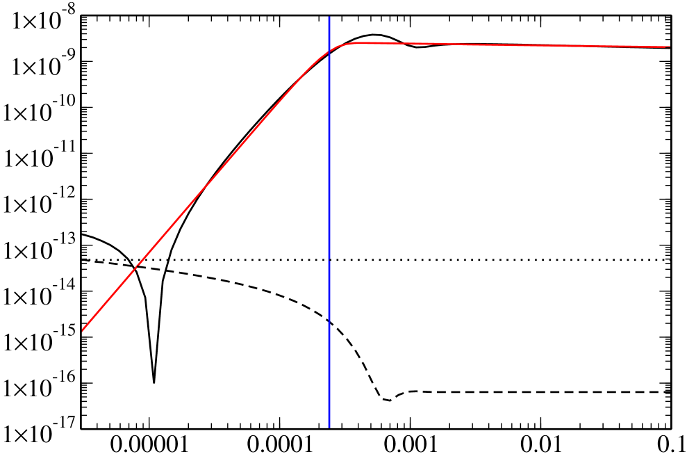
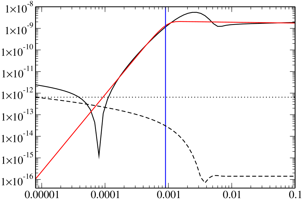
In Fig. 1, we have plotted the scalar and the tensor power spectra for the cases of and . These spectra correspond to the parameters that provide the best fit to the WMAP -year data (for further details, see Ref. pi ). We should mention that in these cases inflation is actually interrupted for about one -fold during the rapid roll regime.
,
,
We had found that, while the case provides a much better fit to the data than the reference concordant model, the case leads to a very poor fit to the data. We believe that the poor fit by the case can be attributed to the large bump in the scalar power spectrum that arises just before it turns nearly scale invariant. Since the bump grows with , we feel that the cases with will fit the data much more poorly and, hence, we have not compared these cases with the data.
The scalar power spectrum with a drop in power at large scales is often approximated by an expression with an exponential cut off of the following form (see, for instance, the first two references in Ref. quadrupole-sic ):
| (9) |
In Fig. 1, we have also plotted this expression for values of , , and that closely approximate the exact spectra we obtain.
In Fig. 2, we have plotted the resulting tensor-to-scalar ratio for the two cases of and .
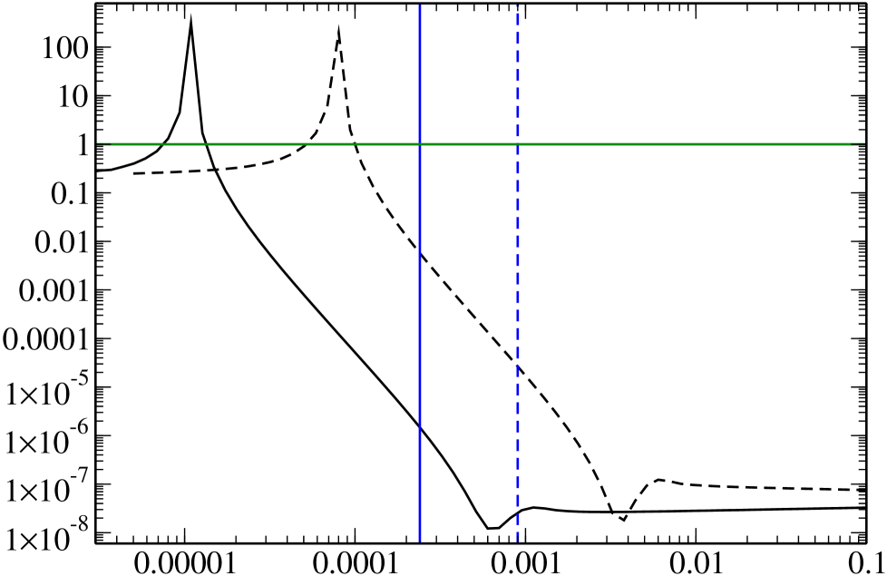
Clearly, the broad characteristics of the scalar and the tensor spectra as well as the tensor-to-scalar ratio that we had outlined in the previous section are corroborated by these two figures.
III.2 A hybrid inflation model
Another model that is known to lead to a punctuated inflationary scenario is a hybrid model that can be effectively described by the following potential (see the first reference in Ref. she ; for the earliest discussion of the model, see Ref. linde-1994 ):
| (10) |
For suitable values of the parameter , this potential admits two stages of slow roll inflation, broken by a brief period of rapid roll. The first slow roll phase is driven by the term and, when has rolled down the potential and has become sufficiently small, the false vacuum term drives the second phase. The parameter determines the amplitude of nearly scale invariant lower step in the scalar spectrum (associated with the modes that leave during the first stage of slow roll inflation), with a mild dependence on . However, very strongly affects the rise in the scalar power (corresponding to the modes that leave just before the rapid roll stage) and the asymptotic spectral index (associated with the modes that leave during the second stage of inflation), since it determines the extent and the duration of the departure from slow roll.
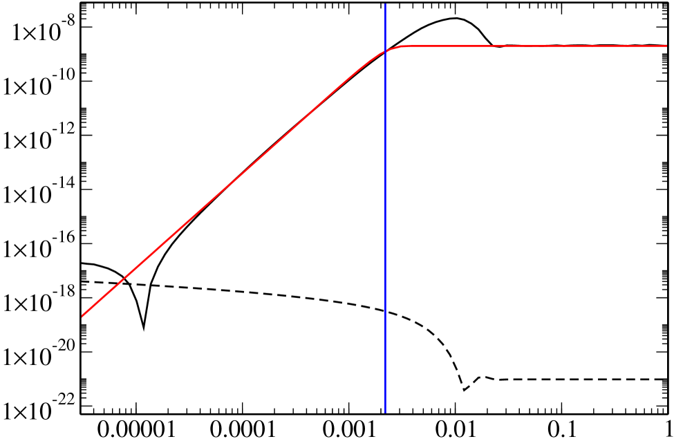
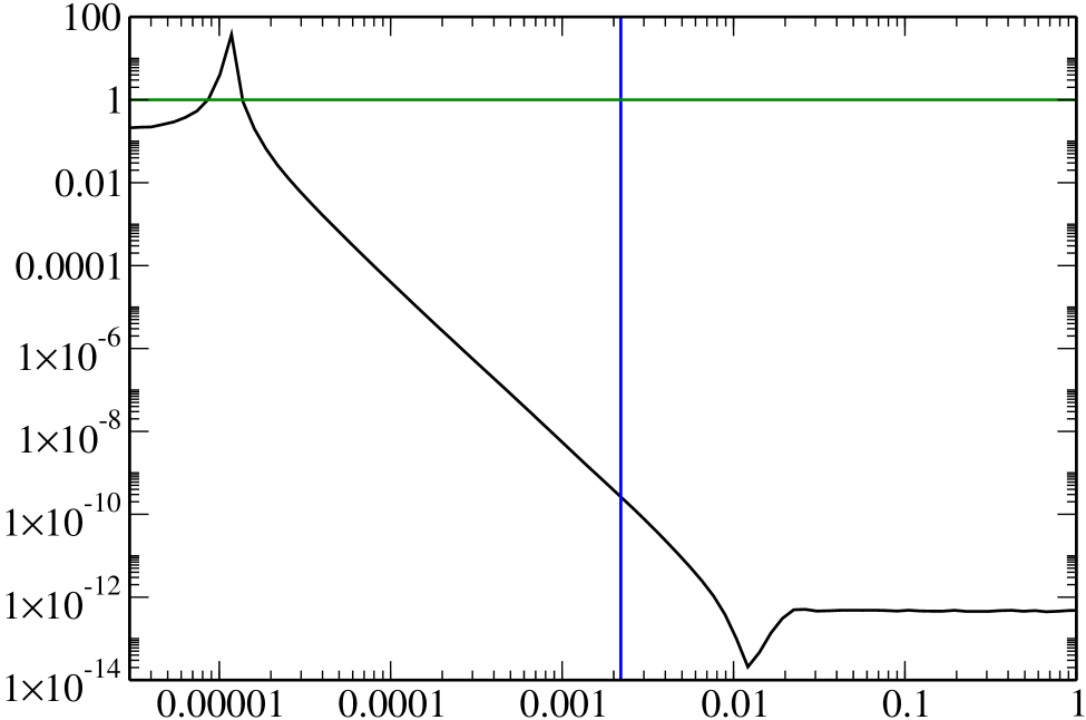
We are able to achieve COBE normalization for a suitable combination of the parameters and . For these values of the parameters, we find that, as in the MSSM-motivated model, a departure from inflation occurs (again, for about one -fold) during the rapid roll phase. In Fig. 3, we have plotted the resulting scalar and the tensor power spectra as well as the associated tensor-to-scalar ratio.
,
We should hasten to clarify that we have not compared the hybrid model with the CMB data, as we had done in the and cases of the MSSM-motivated model. A well known property of the hybrid models is that they lead to blue scalar spectra. We believe that, the blue tilt, along with the rather large bump (which turns out to be larger than the one in , MSSM-motivated model) will considerably spoil the fit to the CMB data.
IV An example of tachyonic punctuated inflation
In this section, we shall consider a tachyonic model that allows punctuated inflation. Since our experience suggests that a point of inflection in the potential is an assured way of achieving a slow-rapid-slow roll transition, we shall construct a tachyonic potential containing a point of inflection.
Tachyonic potentials are usually written in terms of two parameters, say, and , in the following form tachyon ; sami-prava ; steer-2004 :
| (11) |
where is a function which has maximum at the origin and vanishes as . In order to achieve the necessary amount of inflation and the correct amplitude for the scalar perturbations, suitable values for the two parameters and that describe the above potential can be arrived at as follows. One finds that, in these potentials, inflation typically occurs around corresponding to an energy scale of about . Moreover, it turns out that, the quantity has to be much larger than unity (in units wherein ) for the potential slow roll parameters to be small and, thereby ensure that, at least, -folds of inflation takes place. One first chooses a sufficiently large value of by hand in order to guarantee slow roll. The COBE normalization condition for the scalar perturbations then provides the second constraint, thereby determining the values of both the parameters and steer-2004 .
Now, consider a tachyon potential of the form
| (12) |
where . Let the function be defined as an integral of yet another function as follows:
| (13) |
with the constant of integration assumed to be zero. If we choose to be a polynomial that vanishes at least quadratically at a point, say, , then, it is clear that the resulting potential , in addition to satisfying the above mentioned conditions (i.e. having a maxima at the origin and a minima at infinity), will also contain a point of inflection at . A simple function that satisfies our requirements turns out to be777Actually, this function contains another point of inflection at the origin. But, as we shall restrict ourselves to the domain , it is not useful to us.
| (14) |
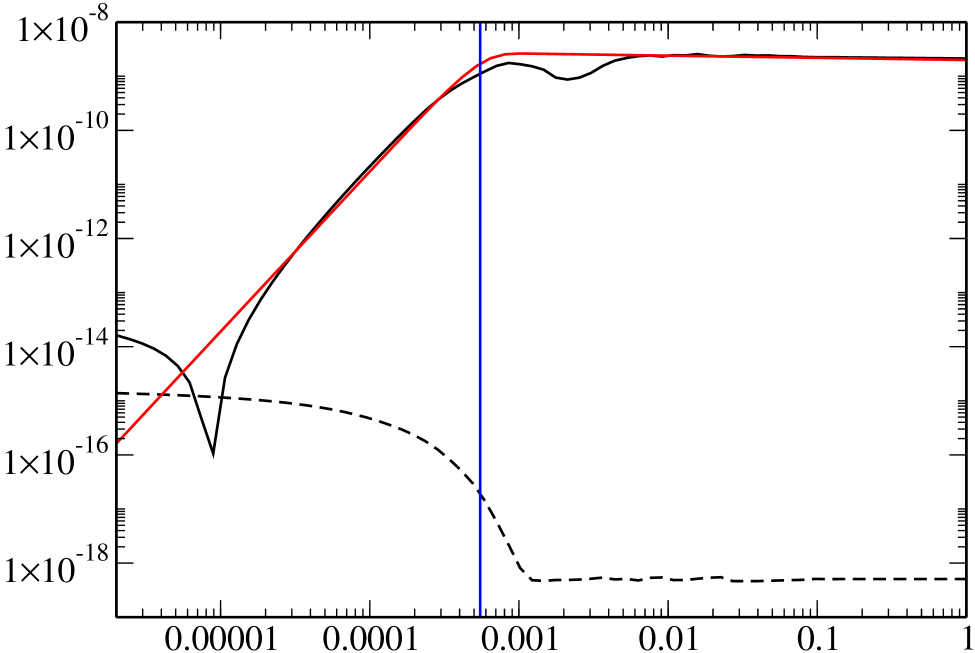
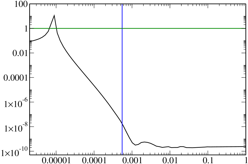
For this choice of the function and appropriate values of the parameters and , we find that the corresponding potential gives rise to punctuated inflation. However, it is important to note that, unlike the earlier examples, the rapid roll phase does not result in a deviation from inflation. In Fig. 4, we have plotted the scalar and the tensor power spectra, and the corresponding tensor-to-scalar ratio that we obtain in this case.
,
It is clear from the figure that the spectra broadly behave in the same fashion as in the earlier examples.
V The effects on the B-modes of the CMB
As is well known, the polarization of the CMB can be decomposed into the E and B-components. While the E-mode polarization is affected by both the scalar as well as the tensor perturbations, the B-modes are generated only by the tensor perturbations888In fact, the B-modes are created by the vector perturbations too. However, inflation does not generate any vector perturbations.. Therefore, the B-mode provides a direct signature of the primordial tensor perturbations (see, for instance, the last reference in Ref. texts ). The detection of the B-mode is a coveted, prime goal of the experimental community (see, for example, the white paper cmbp-dwp ). We feel that the punctuated inflationary scenario can provide additional theoretical motivation for this endeavor.
We have evaluated the angular power spectrum of the B-mode polarization of the CMB (i.e. ) using the Boltzmann code CAMB camb . In Fig. 5, we have plotted for the best fit values of the parameters in the and the cases of the MSSM-motivated model. For comparison, we have also plotted the corresponding angular power spectra for the concordant cosmological model with a strictly scale invariant tensor spectrum and a tensor-to-scalar ratio of , and (the last two values have been chosen since they match the and cases of the MSSM-motivated model at the small angular scales).
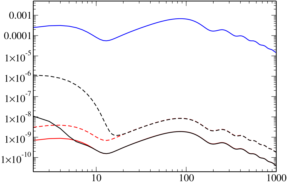
The for the two cases of the MSSM-motivated model clearly exhibit an increase in their amplitude at the lower multipoles, reflecting the rise in the tensor-to-scalar ratio on these scales999We should point out that, in order to evaluate the CMB angular power spectra, CAMB integrates over the following range of wavenumber of the primordial scalar and tensor spectra: . Note that, in both the MSSM-motivated cases, the region where is well beyond the Hubble scale today, viz. (cf. Fig. 2). Therefore, the resulting will be sensitive to the tensor power at such large scales, and we need to be careful about the lower limit of the integral in CAMB. We find that the CAMB’s default lower limit works well in these cases since attains its maximum value at a wavenumber that is larger than the lower limit.. But, despite the rise at the lower multipoles, the amplitude of in these cases proves to be way too smaller than what is possibly detectable in the near future (current/upcoming missions such as PLANCK planck and CMBPol CMBPol are expected to be sensitive to ). However, since the increase in the B-mode power at large angular scales is a generic feature of punctuated inflation, we feel that it improves the possibility that the effect may be detected in the future. It is conceivable that there exist punctuated inflationary models that predict a significantly larger tensor-to-scalar ratio, while still providing a good fit to the CMB temperature angular power spectrum. For example, given a value of the tensor-to-scalar ratio at, say, the Hubble radius today, one can possibly work in the slow roll limit and invert the scalar power spectrum (that results in a good fit) to arrive at a suitable inflationary potential. It seems a worthwhile exercise to systematically hunt for such models.
VI Conclusions
In our earlier work pi , we had performed a Markov Chain Monte Carlo analysis to determine the values of the parameters of the MSSM-motivated model that provide the best fit to the WMAP -year data for the CMB angular power spectrum. We had found that a scalar spectrum in the case leads to a much better fit of the observed data than the spatially flat, CDM model with a power law, primordial spectrum. We should emphasize again that we have not carried out such a comparison with the data for the hybrid or the tachyon model. In the , MSSM-motivated model, we had found that, in addition to the drop in the power at large scales, the bump present in the spectrum before it turns nearly scale invariant had led to the improvement in the fit. In the case, a rather large bump had led to a poor fit to the data. We find that, a similar, large bump arises in the hybrid model as well. Also, as we had mentioned, in the hybrid model, the scalar spectral index proves to be greater than unity at small scales. We feel that these two features will not allow a better fit in the hybrid case. In the tachyonic model, though the spectral index is close to the observed value, we find that no bump (above the asymptotic, nearly scale invariant amplitude) arises in the spectrum. We expect that this feature will spoil the fit to the data. Moreover, we believe that the lack of such a bump is due to the fact that inflation is not interrupted in this case.
In models which start with a period of fast roll, along with the scalar power, the tensor power is also suppressed at large scales nicholson-2008 . But, the drop in the scalar power proves to be sharper than that of the tensors and, as a result, the tensor-to-scalar ratio displays a rise over these scales in such models. It has been argued that such a feature may be detected by ongoing missions such as, for instance, PLANCK planck . We too encounter an increase in the tensor-to-scalar ratio on the large scales, though the reason is somewhat different. In punctuated inflation, the rise in the tensor-to-scalar ratio turns out to be much stronger due to the fact that the tensor amplitude itself increases on large scales. Intriguingly, we find that the rapid rise leads to the tensor-to-scalar ratio being much larger than unity for a small range of modes. However, in the specific models we have considered, the tensor amplitude on scales of cosmological interest (say, ) proves to be too small () for the effect to be possibly detected in the very near future.
The sharper the drop in the scalar spectrum at large scales, the better seems to be the fit to the low CMB quadrupole. In punctuated inflation, the steeper the drop in the scalar power, the faster will be the corresponding rise in the tensor power at large scales. Therefore, if the scalar power drops fast, the tensor-to-scalar ratio can be larger on the small scales, thereby improving the prospects of its detection through the B-modes of the CMB polarization. However, empirical evidence indicates that, in punctuated inflation, a steeper drop in the scalar power requires a larger value of the first slow roll parameter during the rapid roll. But, such a large also leads to a bigger bump (above the asymptotic amplitude) in the scalar spectrum before it turns scale invariant. While a suitable bump seems to provide a better fit to the data at a few lower multipoles after the quadrupole, too large a bump seems to spoil the fit to the data (as in the , MSSM-motivated model). In other words, to lead to a good fit, there appears to be a trade off between the sharpness of the cut off and the size of the bump in the scalar power spectrum. We are currently exploring punctuated inflationary models that will lead to a sufficiently steep drop in the scalar power at large scales, a suitably sized bump at the top of the spectrum, and also a reasonable tensor amplitude at small scales that may be detectable by forthcoming missions.
Acknowledgments
We would like to thank Jinn-Ouk Gong for discussions during the early stages of this work, and for his comments on the manuscript. TS acknowledges enlightening discussions with Alexei Starobinsky. We would also like to acknowledge the use of the high performance computing facilities at the Harish-Chandra Research Institute, Allahabad, India, and at the Korea Institute for Advanced Study, Seoul, Korea.
Appendix A The evolution of the scalar and tensor perturbations for a mode with
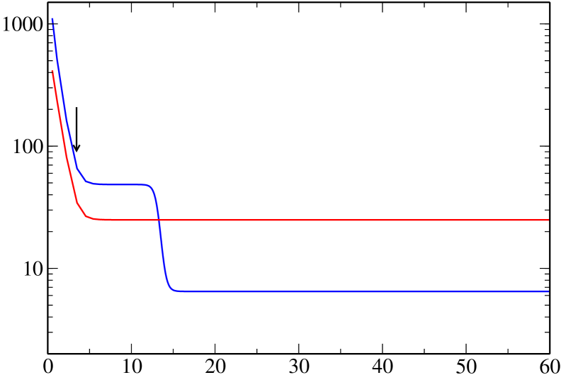
In the various examples of punctuated inflation that we had discussed in the text, though the tensor-to-scalar ratio remains too small () on the scales of cosmological interest, we find that there exists a small range of modes for which the tensor-to-scalar ratio turns out to be greater than unity. We believe that this is an interesting feature with potentially observable consequences. To highlight this feature, in Fig. 6, we have plotted the evolution of the amplitudes of the curvature and the tensor perturbations for a mode that has a tensor-to-scalar ratio greater than unity in the , MSSM-motivated model.
,
Note that, due to the deviation from slow roll, on super-Hubble scales, the amplitude of the curvature perturbation is suppressed when compared to its value near Hubble exit. Whereas, the tensor amplitude approaches a constant value soon after the mode leaves the Hubble radius. It is such a suppression of the curvature perturbation that results in the tensor-to-scalar ratio being greater than unity.
References
- (1) M. R. Nolta et al., Astrophys. J. Suppl. 180, 296 (2009); D. Larson et al., arXiv:1001.4635v1 [astro-ph.CO]; C. L. Bennett et al., arXiv:1001.4758v1 [astro-ph.CO].
- (2) C. L. Bennett et al., Astrophys. J. 436, 423 (1994); E. L. Wright, G. F. Smoot, C. L. Bennett and P. M. Lubin, Astrophys. J. 436, 443 (1994); E. L. Wright, C. L. Bennett, K. Gorski, G. Hinshaw and G. F. Smoot, Astrophys. J. 464, L21 (1996); M. Tegmark, Astrophys. J. Lett. 464, L35 (1996); H. V. Peiris et al., Astrophys. J. Suppl. 148, 213 (2003); M. Tristram et al., Astron. Astrophys. 436, 785 (2005); D. N. Spergel et al., Astrophys. J. Suppl. 170, 377 (2007).
- (3) R. Saha, P. Jain and T. Souradeep, Astrophys. J. 645, L89 (2006); R. Saha, S. Prunet, P. Jain and T. Souradeep, Phys. Rev. D 78, 023003 (2008); P. K. Samal, R. Saha, J. Delabrouille, S. Prunet, P. Jain and T. Souradeep, arXiv:0903.3634 [astro-ph.CO].
- (4) S. L. Bridle, A. M. Lewis, J. Weller and G. Efstathiou, Mon. Not. Roy. Astron. Soc. 342, L72 (2003); P. Mukherjee and Y. Wang, Astrophys. J. 599, 1 (2003); S. Hannestad, JCAP 0404, 002 (2004); A. Shafieloo and T. Souradeep, Phys. Rev. D 70, 043523 (2004); D. Tocchini-Valentini, Y. Hoffman and J. Silk, Mon. Not. Roy. Astron. Soc. 367, 1095 (2006); A. Shafieloo, T. Souradeep, P. Manimaran, P. K. Panigrahi and R. Rangarajan, Phys. Rev. D 75, 123502 (2007); A. Shafieloo and T. Souradeep, ibid. 78, 023511 (2008); R. Nagata and J. Yokoyama, Phys. Rev. D 79, 043010 (2009); G. Nicholson and C. R. Contaldi, JCAP 0907, 011 (2009).
- (5) I. J. O’Dwyer et al., Astrophys. J. 617, L99 (2004); J. Magueijo and R. D. Sorkin, Mon. Not. Roy. Astron. Soc. Lett. 377, L39 (2007); C.-G. Park, C. Park and J. R. Gott III, Astrophys. J. 660 959 (2007); L.-Y. Chiang, P. D. Naselsky and P. Coles, Astrophys. J. 694, 339 (2009).
- (6) Y. P. Jing and L. Z. Fang, Phys. Rev. Lett. 73, 1882 (1994); G. Efsthathiou, Mon. Not. R. Astron. Soc. 343, L95 (2003); J. P. Luminet et al., Nature (London) 425, 593 (2003); A. Hajian and T. Souradeep, Astrophys. J. Lett. 597, L5 (2003); A. Hajian, T. Souradeep and N. Cornish, Astrophys. J. 618, L63 (2005); A. Hajian and T. Souradeep, Phys. Rev. D 74, 123521 (2006); C. Gordon and W. Hu, Phys. Rev. D 70, 083003 (2004).
- (7) J. Yokoyama, Phys. Rev. D 59, 107303 (1999); B. Feng and X. Zhang, Phys. Lett. B 570, 145 (2003); M. Kawasaki and F. Takahashi, Phys. Lett. B 570, 151 (2003); S. Shankaranarayanan and L. Sriramkumar, Phys. Rev. D 70, 123520 (2004); S. Shankaranarayanan and L. Sriramkumar, arXiv:hep-th/0410072; R. Sinha and T. Souradeep, Phys. Rev. D 74, 043518 (2006).
- (8) J. M. Cline, P. Crotty and J. Lesgourgues, JCAP 0309, 010 (2003); C. R. Contaldi, M. Peloso, L. Kofman and A. Linde, JCAP 0307, 002 (2003); L. Sriramkumar and T. Padmanabhan, Phys. Rev. D 71, 103512 (2005); D. Boyanovsky, H. J. de Vega and N. G. Sanchez, Phys. Rev. D 74, 123006 (2006); ibid. 74, 123007 (2006); B. A. Powell and W. H. Kinney, Phys. Rev. D 76, 063512 (2007); C. Destri, H. J. de Vega and N. G. Sanchez, Phys. Rev. D 78, 023013 (2008).
- (9) P. Hunt and S. Sarkar, Phys. Rev. D 70, 103518 (2004); ibid. 76, 123504 (2007); M. Kawasaki, F. Takahashi and T. Takahashi, Phys. Letts. B 605, 223 (2005); J.-O. Gong, JCAP 0507, 015 (2005); L. Covi, J. Hamann, A. Melchiorri, A. Slosar and I. Sorbera, Phys. Rev. D 74, 083509 (2006); J. Hamann, L. Covi, A. Melchiorri and A. Slosar, Phys. Rev. D 76, 023503 (2007); M. Joy, V. Sahni, A. A. Starobinsky, Phys. Rev. D 77, 023514 (2008); M. Joy, A. Shafieloo, V. Sahni, A. A. Starobinsky, JCAP 0906, 028 (2009); M. J. Mortonson, C. Dvorkin, H. V. Peiris and W. Hu, Phys. Rev. D 79, 103519 (2009).
- (10) H. M. Hodges, G. R. Blumenthal, L. A. Kofman and J. R. Primack, Nucl. Phys. B 335, 197 (1990).
- (11) A. A. Starobinsky, Sov. Phys. JETP Lett. 55, 489 (1992).
- (12) V. F. Mukhanov and M. I. Zelnikov, Phys. Lett. B 263, 169 (1991); D. Polarski and A. A. Starobinsky, Nucl. Phys. B 385, 623 (1992); D. Polarski, Phys. Rev. D 49, 6319 (1994); J. A. Adams, G. G. Ross and S. Sarkar, Nucl. Phys. B 503, 405 (1997); J. Lesgourgues, Nucl. Phys. B 582, 593 (2000); J. Barriga, E. Gaztanaga, M. Santos and S. Sarkar, Mon. Not. Roy. Astron. Soc. 324, 977 (2001); Nucl. Phys. Proc. Suppl. 95, 66 (2001); J. A. Adams, B. Cresswell, R. Easther, Phys. Rev. D 64, 123514 (2001).
- (13) R. K. Jain, P. Chingangbam, J.-O. Gong, L. Sriramkumar and T. Souradeep, JCAP 0901, 009 (2009).
- (14) A. A. Starobinsky, Sov. Astron. Lett. 11, 133 (1985); R. Davis, H. M. Hodges, G. F. Smoot, P. J. Steinhardt and M. S. Turner, Phys. Rev. Lett. 69, 1856 (1992); T. Souradeep and V. Sahni, Mod. Phys. Lett. A 7, 3541 (1992); B. C. Friedman, A. Cooray and A. Melchiorri, Phys. Rev. D 74, 123509 (2006).
- (15) G. Nicholson and C. R. Contaldi, JCAP 0801, 002 (2008).
- (16) A. Sen, JHEP 9910, 008 (1999); M. Garousi, Nucl. Phys. B 584 284, (2000); E. Bergshoeff, M. de Roo, T. de Wit, E. Eyras and S. Panda, JHEP 0005, 009 (2000); J. Kluson, Phys. Rev. D 62, 126003 (2000); A. Sen, JHEP 0204, 048 (2002); ibid. 0207, 065 (2002).
- (17) M. Sami, P. Chingangbam and T. Qureshi, Phys. Rev. D 66, 043530 (2002); P. Chingangbam, S. Panda and A. Deshamukhya, JHEP 0502, 052 (2005).
- (18) D. A. Steer and F. Vernizzi, Phys. Rev. D 70, 043527 (2004).
- (19) E. W. Kolb and M. S. Turner, The Early Universe (Addison-Wesley, Redwood City, California, 1990); A. R. Liddle and D. H. Lyth, Cosmological Inflation and Large-Scale Structure (Cambridge University Press, Cambridge, England, 1999); V. F. Mukhanov, Physical Foundations of Cosmology (Cambridge University Press, Cambridge, England, 2005); R. Durrer, The Cosmic Microwave Background (Cambridge University Press, Cambridge, England, 2008).
- (20) H. Kodama and M. Sasaki, Prog. Theor. Phys. Suppl. 78, 1 (1984); V. F. Mukhanov, H. A. Feldman and R. H. Brandenberger, Phys. Rep. 215, 203 (1992); J. E. Lidsey, A. Liddle, E. W. Kolb, E. J. Copeland, T. Barreiro and M. Abney, Rev. Mod. Phys. 69, 373 (1997); B. Bassett, S. Tsujikawa and D. Wands, Rev. Mod. Phys. 78, 537 (2006); W. H. Kinney, arXiv:0902.1529 [astro-ph.CO].
- (21) S. M. Leach and A. R. Liddle, Phys. Rev. D 63, 043508 (2001); S. M. Leach, M. Sasaki, D. Wands and A. R. Liddle, Phys. Rev. D 64, 023512 (2001); R. K. Jain, P. Chingangbam and L. Sriramkumar, JCAP 0710, 003 (2007).
- (22) G. Felder, A. Frolov, L. Kofman and A. Linde, Phys. Rev. D 66, 023507 (2002).
- (23) See, http://www.rssd.esa.int/index.php?project=Planck.
- (24) See, http://cmbpol.uchicago.edu/.
- (25) R. Allahverdi, J. Garcia-Bellido, K. Enqvist and A. Mazumdar Phys. Rev. Lett. 97, 191304 (2006); R. Allahverdi, K. Enqvist, J. Garcia-Bellido, A. Jokinen and A. Mazumdar, JCAP 0706, 019 (2007); J. C. B. Sanchez, K. Dimopoulos and D. H. Lyth, JCAP 0701, 015 (2007); R. Allahverdi, A. Mazumdar and T. Multamaki, arXiv:0712.2031 [astro-ph].
- (26) A. Linde, Phys. Rev. D 49, 748 (1994).
- (27) S. Dodelson et al., arXiv:0902.3796 [astro-ph.CO].
- (28) See, http://camb.info/.