A memory function analysis of non-exponential relaxation in viscous liquids.

Abstract

We analyze data from simulations of two- and three-dimensional (2D and 3D) glass-forming liquids using a correlation function defined in terms of a memory function with a negative inverse power-law tail. The self-intermediate function and the autocorrelation functions of pressure and shear stress are analyzed; the obtained fits are very good, at least as good as with a stretched exponential. In contrast to the stretched exponential, the key shape parameter—the exponent of the power-law tail—seems to be the same for all three correlation functions. It decreases from a value around 2 at high temperature to a value close to 1.58 (2D), 1.50 (3D) at low temperatures. At the same time the amplitude of the tail increases towards towards a limiting value corresponding to a diverging relaxation time, which is related to anomalous diffusion. On the other hand, careful analysis of the long time behavior in the case of the intermediate scattering function suggests that the memory function is cut-off exponentially, which avoids the divergence of the relaxation time. Repeating the fits with an exponential cut-off included indicates that the power-law exponent is in fact independent of temperature and close to 1.58/1.50 over the whole range. Instead of the divergence, a fragile-to-strong crossover in the dynamics, estimated to occur around $T=0.40$ for the 3D Kob-Andersen system. Another key parameter of the fitting procedure may be interpreted as a short-time rate, the amount of decorrelation that occurs in a fixed, relatively short time interval (compared to the alpha time). This quantity is observed to have a near-Arrhenius temperature dependence, while its wavenumber dependence seems to be diffusive ($q^{-2}$) over a wider range than that of the relaxation itself, a further indication that this “bare relaxation rate” is simpler than the full dynamics.

I Introduction

Time-dependent correlation functions are a standard tool for quantifying the dynamics of physical systems.Chaikin and Lubensky (1995) For the most basic analyses, knowledge of a single quantity—the relaxation time—and its dependence on external parameters such as temperature, is sufficient. But often more detailed information, in particular concerning the shape of the correlation function, is required. This might be, for example, because competing theoretical explanations make different predictions about the shape, for example. In the case of highly viscous glass-forming liquidsBrawer (1985); Ediger et al. (1996) some functions typically investigated include the autocorrelation functions of energy, pressure, shear-stress, and dielectric moment. These are related through the fluctuation-dissipation theoremChaikin and Lubensky (1995) to the corresponding dynamic response functions: frequency dependent specific-heat, bulk modulus, shear-modulus (or equivalently viscosity) and dielectric constant, respectively. The key features of viscous-liquid dynamics are (1) the non-Arrhenius temperature dependence of the main, or alpha, relaxation time and (2) the non-exponentiality of the corresponding correlation functions. Any theory of glass-forming liquids has to be able to explain these “nons”—violations of what is generally expected in relaxing systems (Arrhenius temperature dependence and exponential, or Debye, relaxation).

This paper presents a method for fitting relaxation data in the time domain, by parameterizing not the correlation itself but its associated memory function.Boon and Yip (1980) The latter is a unique function related to the correlation function. The motivation comes from the hope that a relatively simple description of the memory function could be attained, and this hope turns out to be justified—very good fits can be achieved by taking the memory function to have the form of an inverse power law for non-zero times. Moreover the exponent of the power law seems to have a common value, approaching at low temperatures a value around 1.6 for the 2D system and 1.5 for the 3D system, for the different correlation functions, something that is not true of the “stretching parameter” $\beta$ when fitting using a stretched exponential. In fact when the memory function parameterization is generalized to include an exponential cut-off, the exponent is temperature independent.

In the next section we discuss some general ideas for describing relaxation and review the concept of the memory function associated with a correlation function. Following that is a brief description of our simulations, while Section IV presents the details of our analysis method as applied to time-domain data from the simulations. Results from the fitting procedure are presented in Section V. Section VI discusses possible ways of interpreting the power-law description.

II Non-exponential relaxation and the memory function

II.1 Correlation functions

In this work we consider normalized correlation functions $\psi(t)$, typically (but not exclusively) defined in terms of a dynamical variable $A(t),$ as

$$\psi(t)\equiv\frac{\langle\Delta A(0)\Delta A(t)\rangle}{\langle(\Delta A(0))^{2}\rangle}.$$ (1)

For example $A(t)$ could be the potential energy, pressure, or shear stress. Here $\Delta$ indicates deviation from the thermal average. Debye relaxation corresponds to a simple exponential decay with time constant $\tau_{D}$:

$$\psi_{D}(t)=\exp(-t/\tau_{D}).$$ (2)

There are many ways to define a relaxation time $\tau_{\alpha}$ which agrees with $\tau_{D}$ in the case of Debye relaxation. For our purposes the most convenient is the time integral of $\psi(t)$:

$$\tau_{\alpha}\equiv\int_{0}^{\infty}\psi(t)dt$$ (3)

One advantage of this definition is that it uses all of the information contained in $\psi(t)$, unlike, for example, a definition based on the time at which $\psi(t)$ attains a certain value. It is also convenient when working with Laplace transforms, since this is simply the the $s=0$ value of the Laplace transform of $\psi(t)$. The function most commonly used to fit time-domain data is the stretched exponential or Kohlrausch-Watt-Williams (KWW)Kohlrausch (1854); Williams and Watts (1970) function,

$$\psi_{KWW}(t)=\exp\left(-(t/\tau_{KWW})^{\beta_{KWW}}\right),$$ (4)

where $\tau_{KWW}$ sets the time scale and $\beta_{KWW}$ is a number between 0 and 1, known as the stretching parameter. Exponential behavior is recovered for $\beta=1$. By integrating we find that $\tau_{\alpha}=\Gamma(1/\beta_{KWW})\tau_{KWW}/\beta_{KWW}$. Fits to Eq. (4) are often very good, but on the other hand experimentsOlsen et al. (2008) suggest that the relaxation crosses over to exponential at the longest times (a decade or more beyond $\tau_{KWW}$), corresponding to the last few percent of relaxation. This has not been investigated much, if at all, in simulations, probably because it is difficult to get high quality data at the longest times. In the case of single-particle diffusion, however, the crossover to exponential behavior should coincide with the onset of Fickian diffusion and the convergence of the van Hove correlation function to a Gaussian, which have been studied by various authors.Szamel and Flenner (2006); Stariolo and Fabricius (2006)

II.2 The memory function

The memory function concept was introduced by the work of ZwanzigZwanzig (1961) and Mori,Mori (1965) which provided a theoretical formalism for the calculation of correlation functions of many-body systems, based on projector-operator techniques. One of the historically most important uses for the memory function has been to elucidate the short-time structure of correlation functions. For example, pure exponential decay, represented by a delta-like memory function, is unphysical at short times, since the correlation, being even and smooth, should have zero slope at $t=0$. Replacing the delta function with a less singular function (for example a step function, a Gaussian, or an exponential) gives more physical short-time behavior. In this work, however, we are concerned with the long time behavior, and in our analysis will ignore the short time behavior, which is mainly associated with vibrational motion and irrelevant for structural relaxation.

The memory function, $K(t)$, is definedBoon and Yip (1980) for a normalized autocorrelation function $\psi(t)$ by

$$\frac{d\psi}{dt}(t)=-\int_{0}^{t}K(t-t^{\prime})\psi(t^{\prime})dt^{\prime}.$$ (5)

The relation between $\psi(t)$ and $K(t)$ is completely invertible, which can be seen by considering the Laplace transformation of this equation:

$$s\tilde{\psi}(s)-1=-\tilde{K}(s)\tilde{\psi}(s),$$ (6)

which implies

$$\tilde{\psi}(s)=\frac{1}{s+\tilde{K}(s)},$$ (7)

an invertible relation between $\tilde{\psi}(s)$ and $\tilde{K}(s)$. Thus we can think of the memory function as a kind of transform of the correlation function. Setting $s=0$ in Eq. (7) gives an expression for $\tau_{\alpha}$:

$$\tau_{\alpha}=\frac{1}{\int_{0}^{\infty}K(t)dt}.$$ (8)

This will be useful below. Although though of our analysis will involve a pure power-law decay of $K(t)$, it should be noted that if $\psi(t)$ is known to decay exponentially at the longest times, the same must be true of the memory function: If $\psi(t)$ decays as an exponentially $\sim\exp(-\lambda t)$ at long times (with $\lambda$ is real and positive), this implies that the least negative singularity of $\tilde{\psi}(s)$ is at $s=-\lambda$. In particular $\tilde{\psi}(s)$ is analytic, as well as real and positive, in a finite region about $s=0$ (recall $\tilde{\psi}(s=0)=\tau_{\alpha}$). The same is true of $1/\tilde{\psi}(s)$ and therefore $\tilde{K}(s)$ (=$1/\tilde{\psi}(s)-s$). Being finite and analytic at $s=0$ is incompatible with a power-law decay for $K(t)$, which would correspond to a power-law for $\tilde{K}(s)$ with (in general) non-integer exponent as $s\rightarrow 0$. If an exponential cut-off is included in $K(t)$, however, this moves the singular point a finite distance to the left along the negative real $s$-axis.

II.3 Interpretation as a rate

A useful starting point for considering the meaning of $K(t)$ is the case $K(t)=\gamma\delta(t)$, which gives exponential relaxation $\psi(t)=\exp(-\gamma t)$, i.e., $\tau_{\alpha}=1/\gamma$, consistent with Eq. (8). This is the memory-less, or Markov, case. Note that the ‘amplitude’ $\gamma$ gives the rate of the exponential decay. Consider integrating Eq. (5) as if it were a physical equation of motion: In the memoryless case, as time goes on, the delta function means that the only contribution to the integral on the right-hand side is from the current time, $t^{\prime}=t$. Thus, the rate of change of $\psi(t)$ is proportional to its current value and independent of its previous values. This of course gives exponential relaxation. If we generalize slightly to the case $K(t)=K$, a constant, for $t<T$, and zero otherwise, then for times much greater than $T$ we again expect exponential decay with relaxation time $\tau_{\alpha}=1/(KT)$. When $K(t)$ is non-zero for all $t>0$, but $\int_{0}^{t}K(t^{\prime})dt^{\prime}$ converges sufficiently quickly (e.g. exponentially) to a finite positive value, we can expect exponential decay in $\psi(t)$ for long times.

For times $t$ when the memory function is still changing, $\int_{0}^{t}K(t^{\prime})dt^{\prime}$ gives an estimate of the instantaneous decay rate of $\psi(t)$. What happens when $K(t)$, which must be positive at time zero (otherwise $\psi(t)$ will diverge), becomes negative? At that point $\int_{0}^{t}K(t^{\prime})dt^{\prime}$ starts to decrease, implying that the decay rate decreases. As long as $K(t)<0$, $\psi(t)$ will exhibit slower-than-exponential relaxation—the instantaneous decay rate keeps decreasing. Therefore we expect that for viscous liquids the memory function is negative and significant for times up to $\tau_{\alpha}$, around which time $\int_{0}^{t}K(t^{\prime})dt^{\prime}$ has more or less converged to the limiting value and exponential relaxation takes over.

II.4 Discrete memory function

When we consider simulation data we will be not interested in short-time vibrational contributions to $\psi(t)$ or $K(t)$. A standard way of removing the effects of vibrations is to consider the so-called inherent dynamics,Stillinger (1995) obtained by minimizing configurations along the actual simulated trajectory to the corresponding local minimum of the potential energy—the inherent state. The correspondence is defined by steepest-descent minimization and is, in principle, unique for almost all configurations. It has been shown that the resulting trajectory of inherent states preserves the long time features of the dynamics. Schrøder et al. (2000); Liao and S.-H.Chen (2001) Correlation functions are essentially unchanged except that the usual initial decay due to vibrations on the picosecond time scale is missing. A technical problem is introduced by this procedure, however: The inherent correlation functions tend to have non-zero, and therefore discontinuous, slopes at $t=0$. This is not so surprising, given that the inherent trajectory is itself necessarily discontinuous, but it does pose problems for defining the short-time behavior of the memory function. To avoid these problems, and given that simulation data is generally available at regular, discrete times, we write a discrete version of Eq. (5):

$$\psi_{n+1}-\psi_{n}=-\sum_{m=0}^{n}K_{n-m}\psi_{m}.$$ (9)

Here time has been discretized in units of $\Delta t$, so $\psi_{n}\equiv\psi(t=n\Delta t)$. Equation (9) can be straightforwardly used to calculate the discrete values of the autocorrelation function, $\{\psi_{n}\},n\geq 0$, given the discrete values of the memory function, $\{K_{m}\},m\geq 0$: Start by setting $\psi_{0}=1$ and then for each $n>0$ in turn, calculate the sum on the right hand side, which only involves $\psi_{m}$ for $m\leq n$ and the known $\{K_{m}\}$, to get the next unknown value, $\psi_{n+1}$. It is almost as straightforward to see that the reverse transformation is possible, i.e., given $\{\psi_{n}\},n\geq 0$, to determine $\{K_{m}\},m\geq 0$. For example, from Eq. (9) for $n=0$ one finds

$$K_{0}=1-\psi_{1}/\psi_{0}=1-\psi_{1},$$ (10)

(since we assume the normalization $\psi_{0}=1$). Knowing now $K_{0}$, writing Eq. (9) for $n=1$ gives again an equation with only one unknown, namely $K_{1}$. In this way the values of $K_{m}$ can be solved for one by one. This process may be formalized using the idea of a generating function.Wilf (1994) We consider the series $\{\psi_{n}\}$ as the coefficients of a power series in a variable $z$, which (formally) defines the so-called generating function $\psi(z)\equiv\sum_{0}^{\infty}\psi_{m}z^{m}$, similarly $K(z)\equiv\sum_{0}^{\infty}K_{m}z^{m}$. We may treat generating functions as quantities which can be added, multiplied and divided (providing the first coefficient is non-zero), and thus can note that the right hand of Eq. (9) is in fact the $n$th coefficient in the product series $-K(z)\psi(z)$ (this is like the convolution-product correspondence in Laplace transforms). Thus the equation may be re-written as

$$(\Delta\psi)(z)=-K(z)\psi(z),$$ (11)

where the difference function $(\Delta\psi)(z)$ is defined as the series $(\Delta\psi)_{0}=0$, $(\Delta\psi)_{n}=\psi_{n}-\psi_{n-1},n>0$. $K(z)$ is then given by

$$K(z)=-\left(\frac{1}{\psi(z)}\right)(\Delta\psi)(z),$$ (12)

which may be evaluated using standard algorithms for multiplying and dividing power series.Wilf (1994) Mathematically this procedure is equivalent to the inversion procedure mentioned above; thinking in terms of generating functions simply makes the implementation more straightforward. We use this transformation in the data analysis to relate correlation functions to their corresponding memory functions. In the following, we use $K(t)$ to mean $K_{m}/(\Delta t)^{2}$, where $t=m\Delta t$.

III Simulations

III.1 Systems and potentials

We have simulated both two- and three-dimensional (2D and 3D) binary Lennard-Jones (BLJ) fluids. The parameters for the BLJ potential for both 2D and 3D are (where L and S stand for large and small particles, and $\epsilon$ and $\sigma$ the energy and length scales, respectively) $\epsilon_{LL}=1$, $\epsilon_{SS}=0.5$, $\epsilon_{LS}=1.5$, $\sigma_{LL}=1$, $\sigma_{SS}=0.88$, $\sigma_{LS}=0.8$. All particles have the same mass $m=1$. These parameters are identical to those of the 3D BLJ introduced by Kob and Andersen Kob and Andersen (1994). The potential was truncated using an interpolating polynomial between 2.4 $\sigma_{\alpha\beta}$ and 2.7 $\sigma_{\alpha\beta}$ ($\alpha,\beta\in\{L,S\}$). In all simulations periodic boundary conditions with constant area/volume were used. In 2D the total number of particles $N_{p}$=700 of which 60% were of type L, while in 3D, $N_{p}$=1372 of which 80% were of type L. The particle density was 1.2$\sigma_{LL}^{-d}$ in both cases (where $d$ is the dimension). Constant energy dynamics were simulated using the Verlet algorithm with a time step of 0.01 $\sigma_{LL}\sqrt{m/\epsilon_{LL}}$ From now on, all quantities will be reported in the units defined by $\epsilon_{LL}$, $\sigma_{LL}$ and $m$. If one converts to physical units by assuming that the parameters for large particles are chosen to model Argon (i.e., $\sigma_{LL}=0.34$ nm, $\epsilon_{LL}=997$ kJ/mol, $m=39.95$ u), then the time unit corresponds roughly to 2 ps.

III.2 Runs

Initial configurations consisted of fcc lattices with particles randomly assigned to be of type L or S such that the appropriate fraction was achieved. All simulations were at constant NVE; in particular the energy was controlled rather than the temperature $T$, but we quote the temperature defined in terms of the mean kinetic energy per particle instead as it is more meaningful. Starting at at $T\sim 1.0$ (where the liquid is not particularly viscous) ten independent runs (differing by the random placement of the particles on the initial lattice) were made. The initial lattices melted immediately and equilibrated in the liquid state. For each state point, an equilibration run was carried out followed by a production run of the same length. Equilibration was checked by examining the self-intermediate scattering function $F(q_{m},t)$ for the larger particles; $q_{m}$ is 6.5 in 2D and 7.3 in 3D (corresponding roughly to the peak of the structure factor for large particles). $F(q_{m},t)$ was required to be essentially the same for all ten runs, and the run-length to be of order 100 times the structural relaxation time ($\tau_{\alpha}\equiv\int_{0}^{\infty}F(q_{m},t)dt$). If the condition was not satisfied, the production run was considered to be part of the equilibration and a new production run was initiated from the final configurations. Steps in temperature were made by changing the total energy according to the estimated specific heat; a new kinetic energy was chosen such that when summed with the current potential energy the correct total energy would result. Then the particles’ velocities were randomized using a Gaussian distribution with the appropriate width and then rescaling to give the exact desired kinetic energy. During the equilibration process it was checked that the new temperature (mean kinetic energy) was the desired one and velocities were rescaled if necessary (generally a small change).

III.3 Calculating correlation functions

During the simulations, collective quantities such as potential and kinetic energy and the different components of stress were computed and written at regular intervals (typically every 100 or 500 time steps, though some shorter runs were made with more frequent output in order to determine the short time behavior of the correlation functions). Configurations were saved at “logarithmic intervals” to allow calculation of $F(q,t)$ for a broad range of times $t$ without writing configurations as frequently as the collective quantities (which would require a huge amount of disk storage). Because $F(q,t)$ involves an average over particles, it has significantly smaller statistical error and therefore has low noise out to quite long times beyond the relaxation time. It should be noted, however, that it is technically not the autocorrelation function of a dynamical variable. Autocorrelation functions of collective quantities were calculated using standard Fourier transform techniques. Both these and $F(q,t)$ were averaged over the ten runs. For the main part of the analysis the autocorrelation functions were also “logarithmically averaged” in time. This weights different time scales equally and involves grouping the data points into equal-sized bins of $\log(t)$, and averaging within each bin.

III.4 Inherent states

Some of the analysis was carried on inherent-state configurations. The method used to minimize the energy was a combination of “molecular dynamics minimization”Stoltze (1997) and conjugate gradient.Press et al. (1987) This combination has been found to reduce the possibility of finding the “wrong” minimum, which can happen if conjugate gradient alone is used.Bailey et al. (2009) Configurations were minimized every 10, 100 or 1000 configurations—more frequent minimization enables resolution of shorter time scales, but longer time scales cannot be accurately probed.

IV Data analysis: Determining $K(t)$

Figure 1: (Color online) Left panel, shear stress (unnormalized) autocorrelation function for true and inherent dynamics. They differ only at short times. The slight dip in the curve for true dynamics at $t=5$ is from combining separate short- and long- time simulations. Minimization was carried out every ten time steps, which defines the resolution of the memory function, $\Delta t=10dt=0.1$. The dashed line shows the correlation function obtained from attempting to invert the attempted fit to the memory function, while the dotted line shows that obtained by inverting using the exact memory function truncated at $t=100$. Right panel, memory function for the inherent shear-stress autocorrelation function. Inset shows the negative tail in a double-logarithmic plot, along with a power-law fit.

IV.1 Inversion of the correlation function to get the exact $K(t)$

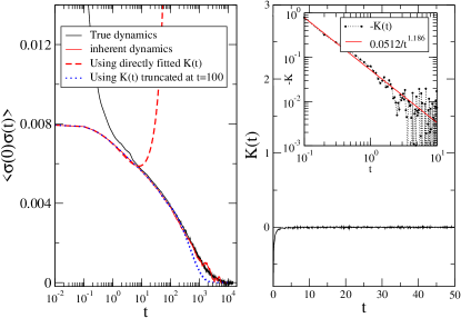
We start by applying the transformation described above to the simulation data. Fig. 1 shows the 2D, T=0.34 shear-stress autocorrelation function for both true and inherent dynamics. The agreement between the two at long times is clear, although there is more noise in the inherent case—due to the cost of minimization, not as long times can be simulated. The right panel of Fig. 1 shows the result of the discrete memory transform. Recall that this returns the exact memory function $K(t)$ for the data. This is positive at $t=0$, but negative for all $t>0$ (note that $t$ really means $n\Delta t$ for an integer $n$; since minimization was carried out every ten time steps, $\Delta t=0.1$). As shown in the inset, the data suggest an inverse power-law for the negative tail, although the noise is too great to justify this for $t>2$, a very short time compared to the relaxation time $\tau_{\alpha}\sim 3000$. Nevertheless let us attempt a fit to a simple power-law in the hope that this is in fact the correct form of $K(t)$ for $t>0$. The fit yields the expression $0.0512/t^{1.186}$ for $K(t)$. Testing whether this expression is in fact a good representation of the true memory function is simple: we simply use Eq. (9) to construct the correlation function corresponding to the fitted $K(t)$. The value of $K_{0}$ is not fit; rather the exact value from the inversion is used. The result, shown as the dashed line in the left panel of Fig. 1, is a disaster: after reasonable agreement up to $t\sim 10$, the transformed $\psi(t)$ stops decaying and in fact begins to increase and eventually diverges. The problem can actually be foreseen by considering the time integral of $K(t)$, which in the discrete case is the sum $\sum_{n}K_{n}/\Delta t$. The value of $K_{0}(=1-\psi_{1})$ here is 0.0286, so that its contribution to the sum is 0.286. The sum over the power-law part requires the evaluation of the Riemann zeta function $\zeta(s)$ at $s=1.186$, which is estimated numerically to be 5.97. Including the appropriate factors of $\Delta t$ and the prefactor yields the contribution from the power law to be -0.469, making the whole sum negative. Moreover the sum first becomes negative around where the inverted correlation function begins to increase–at this point the effective decay rate has become negative, and so the correlation function grows rather than decays.

Clearly, direct fitting of the memory function is problematic. The fit which applies at least up to $t\sim 2$ clearly is wrong for $t>10$. Because the noise in the exact memory function is so much larger than the true value, standard fitting procedures cannot distinguish it from zero in this region. On the other hand, we can directly check that it is indeed significantly different from zero for quite long times: Taking the exact memory function, but setting it to zero for times greater than $t=100$, and inverting, we find the correlation function indicated by the dotted line in Fig. 1. After $t\sim 500$ it drops below the true correlation function in a more or less exponential fashion, as expected when the memory function is only non-zero for a finite range of time. Thus the apparent power-law behavior at short times must cross over to something more rapidly decaying, but still significantly different from zero.

Figure 2: Main figure, fitted memory function consisting of an inverse power-law multiplied by a piecewise linear function. Inset, comparison of the shear stress autocorrelation function from simulations and the correlation function corresponding to the fitted memory function. In this case the correlation function was a combination of that determined by inherent dynamics at short time and that determined by real dynamics at long-time, in order to have a more accurate and less noisy curve at long times.

IV.2 Matching the correlation function by fitting $K(t)$.

An approach other than direct fitting of the exact $K(t)$ is clearly needed. Since the noise in the correlation function is small compared to the function itself, comparing this to a trial function in a fitting procedure will not suffer the same problem. This suggests a practical method for determining the memory function: We choose a functional form which is quite flexible, containing many parameters. For any given set of parameter values we can generate the corresponding trial correlation function which can be compared in a least-squares sense to the actual correlation function. Then we vary the parameters to optimize the match.

The value of $K_{0}$ is fixed from the start to $1-\psi_{1}$. Given that the exact $K(t)$ seems to have an initial inverse power-law decay for $t>0$, we start with such a function. To provide flexibility we multiply by a piecewise linear function; such a function will have discontinuous changes in slope but is simple and general—and hopefully the dominant behavior has been captured by the power-law factor. Thus this general fitting form $K_{gen}(t)$ is

$$K_{gen}(t)=-\frac{A}{t^{\alpha}}L(t),t>0$$ (13)

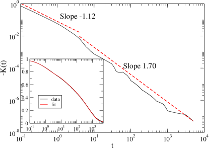
where $L(t)$ is a piecewise linear function defined by a set of nodes $t_{k}$ and values $L_{k}$ for $k=0,1,2,\ldots,n_{nodes}$. The first node is at $t=0$, i.e., $t_{0}=0$ and $L_{0}$ is fixed at unity. We choose $n_{nodes}\sim 20$ to provide sufficient flexibility; a typical set of node locations $t_{k}$ is 0, 1, 2, 4, 5, 6, 8, 10, 20, 30, 40, 50, 60, 80, 100, 200, 500, 750, 1000, 3000, 5000. The adjustable parameters are then the overall coefficient $A$, the exponent $\alpha$, and the coefficients $L_{k}$, $k=1,\ldots,n_{nodes}$. At this stage we do not seek the true functional form of $K(t)$; rather, we wish to have a fairly accurate representation which is relatively free of noise. To obtain the optimal parameter values in $K_{gen}(t)$, a conjugate-gradient procedure is used. Some details of this are given in the appendix. Fig. 2 shows the result of this procedure. While the discreteness due to the piecewise linear function is clearly visible, the overall form is clear. In particular, there is a clear cross-over at around $t=5$ from the power law we initially identified to a more rapidly decaying power law, with exponent $\sim$1.7. This cross-over means that the time integral converges to a positive value and the effective decay rate never becomes negative.

Figure 3: . (Color online) Comparison of autocorrelation function and fit with a memory function involving a single inverse power law in the tail. The data is the same as in Fig. 2, but only times which were multiples of 10 were included. The fitted exponent was 1.84, reasonably close to the apparent exponent of 1.7 observed in Fig. 2.

IV.3 Simple power-law form for $K(t)$ for $t>10$.

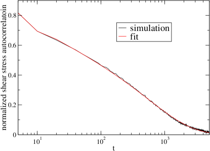
The observation that $K(t)$ is well approximated by a single inverse power law for times greater than about 5 immediately suggests a simplification: If we choose to not resolve times shorter than this, a fit using only a single power law for the non-zero part of $K(t)$ may be possible. Fig. 3 shows that this is indeed true. Here times greater than 10 were included, corresponding to sampling at an interval $\Delta t=10$. This time scale is also significant for another reason (not necessarily unrelated): It corresponds to the end of the vibrational contribution to the stress autocorrelation function of the true dynamics (see left panel of Fig. 1). This suggests that we can avoid the time consuming energy minimization process altogether and use only the data from the true dynamics. There is one problem, though: We cannot get the $t=0$ value of the (inherent) autocorrelation function from the true dynamics. To get around this we leave it as a fitting parameter; this gives us a procedure for fitting autocorrelation functions with three parameters: $R_{01}\equiv\psi_{0}/\psi_{1}$, $A$ and $\alpha$. Note that $R_{01}$ is directly related to $K_{0}$, so one could equivalently think of $K_{0}$ as the parameter. This fitting function involving a single inverse power law has been used in most of the analysis.

It is convenient to represent that amplitude of the power-law in terms of a “tail-weight fraction” $f$, defined such that $f=1$ corresponds to the limiting case where the sum over the whole negative ($m>0$) part of $K_{m}$ exactly cancels the positive contribution from $K_{0}$. Thus we represent $K_{m}$ for $m>0$ as

$$K_{m}=-K_{0}\frac{f}{\zeta(\alpha)}\frac{1}{m^{\alpha}},m>0,$$ (14)

where $\zeta(\alpha)\equiv\sum_{n=1}^{\infty}1/n^{\alpha}$ is the Riemann zeta-function. Then the relaxation time is given simply by

$$\tau=\frac{1}{\sum_{n}(K_{n}/(\Delta t)^{2})\Delta t}=\frac{1}{K_{0}\Delta t}\frac{1}{1-f}$$ (15)

This form makes explicit a few things: for near zero $f$, the relaxation rate is essentially the inverse of $K_{0}$. As $f$ increases the negative tail “cancels out” part of the latter, increasing the relaxation time, and the limit $f\rightarrow 1$ gives a diverging relaxation time.

Figure 4: (Color online) Main figure, examples of fits using the 3-parameter power-law form of $K(t)$ to three correlation functions calculated from simulations of the Kob-Andersen binary Lennard-Jones mixture in 3D at $T$=0.46. Solid lines: data; dashed lines: fits. In contrast to Fig. 3, logarithmic binning/averaging was used for the shear stress and pressure autocorrelation functions.

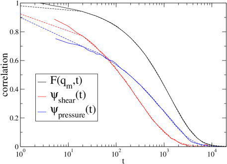
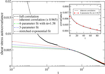
Examples of fits to the three functions, $F(q_{m},t)$ and the shear stress and pressure autocorrelation functions, are shown in the main part of Fig. 4 for one temperature in the 3D system. Here and in the all the analysis presented below, the discretization interval was $\Delta t$=20.

IV.4 Long-time behavior: An exponential cut-off in $K(t)$

Figure 5: (Color online) Comparison of memory functions obtained for intermediate scattering function (3D, $T=0.46$, $\tau_{\alpha}=1500$) using 3- and 4-parameter fits. The exponential cut-off in the latter is clearly visible. Inset, comparison of the correlation functions from the fit with the data, along with a stretched exponential. Here a double-log scale is used to emphasize the long-time behavior (the differences would not be visible otherwise).

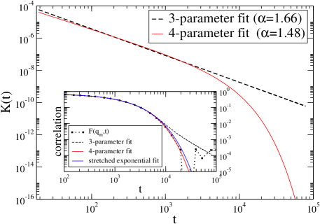
As mentioned in Section II, experimentsOlsen et al. (2008) suggest that autocorrelation functions switch over to exponential decay at very long times. This is incompatible with the fitting function we have identified—as discussed in Section II, power-law decay of $K(t)$ corresponds to a power-law singularity in $\tilde{K}(s)$ as $s\rightarrow 0$, implying non-analyticity of $\tilde{\psi}(s)$ in the same limit, which excludes exponential behavior of $K(t)$ at long times. Thus we should—in principle at least—allow the possibility of including an exponential cut-off in the fitting function for $K(t)$. The question is whether the available data requires it to get a satisfactory fit. Only in the case of the intermediate scattering function is the noise sufficiently low to allow investigation of the long time behavior (when the correlation function has decayed to less than 1% of its original value). Fig. 5 compares the three-parameter fit using Eq. 14 with a 4-parameter fit involving an exponential cut-off:

$$K_{m}=-K_{0}\frac{f}{\zeta(\alpha)}\frac{\exp(-m\Delta t/\tau_{c})}{m^{\alpha}},m>0$$ (16)

where $\tau_{c}$ is the characteristic time of the exponential cut-off. The memory functions are shown in the main part of the figure, while the correlation functions are shown in the inset. For comparison, a stretched-exponential fit is also included. The three-parameter (pure power-law) memory-function fit noticeably underestimates the decay rate at long times. Including the cut-off gives a much better fit, although some improvement is of course expected due to the extra parameter). Notice that the stretched exponential function fits also better than the pure power-law fit at long times, as well as the cut-off memory function. For the shear stress and pressure autocorrelation functions the long time data is not good enough to warrant including the exponential cut-off as a fourth parameter, although we shall see that it can make sense to do so when there is reason to fix the exponent $\alpha$ to a particular value. In the following, “four-parameter” and “three-parameter” fits refer respectively to whether the exponential cut-off was included or not, regardless of whether one or more of those parameters was constrained in the fitting process.

V Results

V.1 Relaxation times

Figure 6: Arrhenius plot of relaxation times for structure ($F(q_{m},t)$), shear stress and pressure autocorrelation functions, for 2D and 3D data (closed symbol), determined by summing the fitted normalized memory function.

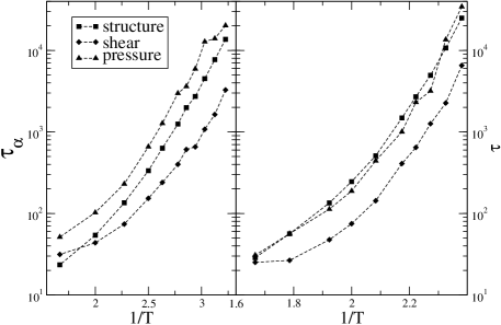
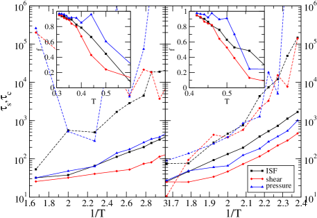
We start by presenting the relaxation times $\tau_{\alpha}$ for the different correlation functions. As stated earlier, we define $\tau_{\alpha}$ as the integral of the normalized correlation function. With simulation data there is a contribution at short times due to vibrations. The relative height of this varies among the different correlation functions, making the choice of normalization problematic. In principle this can be removed by considering correlation functions of inherent quantities, but the time taken for quenches means that determining the correlation function accurately at long times is difficult. We avoid these problems by using the fitted correlation functions, normalizing by the zero-time value that emerges from the fitting process. To be consistent with the discrete-time formalism for dealing with the memory function we sum the correlation functions and multiply by $\Delta t$, rather than integrating them. This makes a positive difference of order $\Delta t/2$, negligible except when the relaxation time is of order $\Delta t$. This is the case at the highest temperatures, particularly for shear stress (note the upwards bend in the relaxation time curve at the extreme left of the plot). The value of $\tau_{\alpha}$ determined from the fit varies only slightly according to whether the 3- or 4- parameter fitting function for $K(t)$ is used. Fig. 6 shows Arrhenius plots for both 2D and 3D systems of the three correlation functions investigated. Some curvature—corresponding to so-called “fragility” of the viscous liquid—is evident, although less so in the 2D data. In both 2D and 3D the shear relaxation time is noticeably shorter than those of pressure and structural relaxation ($F(q_{m},t)$). The pressure relaxation time tracks closely the structural one in 3D, but exceeds it noticeably in 2D. In fact the difference between pressure and shear stress relaxation in 2D is of order a factor of ten; in 3D it is closer to a factor of four. Note that at higher temperatures (0.5–0.6) the relaxation time is of the same order as the discretization interval $\Delta t=20$, so a large part of the relaxation actually takes place within the first interval. Unsurprisingly, this limits the ability of the fitting procedure to accurately determine the zero-time value which leads to errors in normalization and hence in $\tau_{\alpha}$, particularly for the collective correlation functions of pressure and shear stress where the noise is high. In these cases a fit to a stretched exponential was made first, which was then used for the memory function fit. We note finally that is apparently nothing special happening around the mode-coupling temperature $T_{c}=0.435$ previously identified for the 3D Kob-Andersen system (albeit with a slightly different cut-off in the potential).

V.2 Short-time rate $K_{0}$ and corresponding time $\tau_{s}$

Figure 7: Arrhenius plot of the inverse short-time rate $\tau_{s}=\Delta t/K_{0}$ determined from different fits to $F(q_{m},t)$, compared with the relaxation time $\tau_{\alpha}$, and the cut-off time $\tau_{s}$ of the 4-parameter fit, for 2D (left panel) and 3D (right panel) systems. The data labelled “3-parameter (cons.)” refers to simultaneous fits of the three correlation functions at a given temperature, constraining the exponent $\alpha$ to be the same in all three.

Figure 8: (Color online) Comparison of inverse short-time rate $\tau_{s}=\Delta t/K_{0}$ for different kinds of correlation functions. Left and right panels show 2D and 3D data, respectively. Upper panels show the results of fitting each curve separately; lower panels show the results of constraining the power-law exponent $\alpha$ to be the same for all three curves at a given temperature.

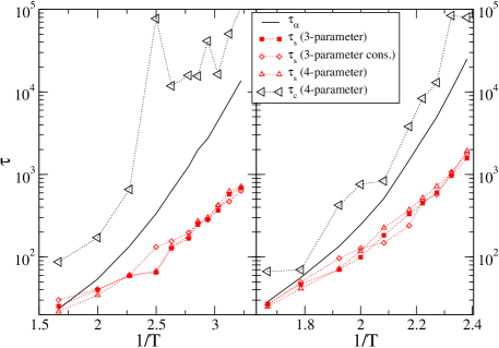
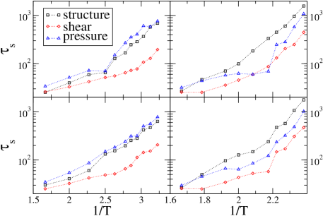
We now investigate the parameters determined by the fitting procedure starting with the temperature dependence of the parameter $K_{0}$, related to the short-time relaxation rate. More precisely, we consider $\tau_{s}\equiv\Delta t/K_{0}$, which is an effective time scale quantifying the amount of relaxation that occurs over the interval $\Delta t$, a “short-time relaxation time”. This is plotted Figure 7 along with $\tau_{\alpha}$ for $F(q_{m},t)$. Results of three different fitting schemes are shown: three-parameter fit, four-parameter fit (i.e., including the exponential cut-off) and a three-parameter fit where the exponent $\alpha$ is constrained to be equal for the three correlation functions at a given temperature. The motivation for the latter will become clear later on. The variation between the different fits gives an estimation of the error bars on this quantity. $\tau_{s}$ is less than $\tau_{\alpha}$, which is necessarily the case if $K_{m}<0$ for $m>0$. The main point is that $\tau_{\alpha}$ is more or less equal to the $\tau_{s}$ at high temperatures—something necessarily true for exponential relaxation—but increases relative to it as temperature decreases. The temperature dependence of the $\tau_{s}$ is activated, which is to say it is at least Arrhenius. The data in the figure are not precise enough to determine whether the rate is super-Arrhenius, but certainly the effective barrier (the slope in the figure) is lower than for $\tau_{\alpha}$ itself. Figure 8 shows comparison of $\tau_{s}$ for the three different quantities. The upper panels represent independent fits, while the lower ones represent constrained fits where $\alpha$ is the same for the three quantities.

V.3 Power-law exponent $\alpha$

Figure 9: (Color online) Temperature dependence of the exponent $\alpha$ for different quantities in 2D (left panels) and 3D (right panels) simulations. Upper panels show the result of independently fitting the different correlation functions; lower panels show the common exponent obtained by constraining it to be the same for all three, and that obtained in the (unconstrained) four-parameter fits to $F(q_{m},t)$. In both systems, $T=$0.6 values are from fits using $\Delta t=$10. The horizontal lines indicate $\alpha=$1.5.

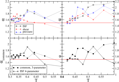
Figure 9 shows the temperature dependence of the power-law exponent $\alpha$ for the two different systems, the three different correlation functions, and for different fitting schemes. Considering first the top two panels, the interesting feature is that the exponent values seem to converge as the temperature is lowered, towards $\sim$1.6 in 2D and $\sim$1.5 in 3D. At higher temperatures there is significant scatter, and, for the 3D case at least, generally higher values up to around 2. The apparent convergence at low temperatures suggests that perhaps the true values of the exponents are in fact equal for the three functions at each temperature; the scatter in the unconstrained fits would then be understood to be due to noise in the data. We therefore attempted a fit where $\alpha$ is constrained to be the same for all three correlation functions. In most cases the quality of the fit is indistinguishable by eye from the unconstrained fit (not shown). The exceptions are some fits to $F(q_{m},t)$ in 2D where the constrained fit tends to reduce the value of $\alpha$ compared to the unconstrained fit, which results in a somewhat slower decay at long times (this could be probably compensated for by including the exponential cut-off, as explained in the following paragraph; we have not done this). The temperature dependence of the constrained-$\alpha$ is more or less similar to the constrained case for the 3D data, while noticeably reduced in the 2D case. The effect on the constrained fit on the values of $\tau_{s}$ can be seen in the lower panels of Fig. 8. There is a tendency towards smoother temperature dependence, which supports the idea that a constrained fit can yield more accurate results because the tendency to fit noise in any one of the curves is limited by the constraint. On the other hand the temperature dependence of $\tau_{s}$ for the intermediate scattering function is actually less smooth in the constrained fit it has been “infected” by the greater noise in the collective functions. In principle this could be compensated for assigning a greater weight to the intermediate scattering function due to the smaller noise. This has not been attempted; it would require an unbiased estimate of the errors on the correlation functions.

Also shown in the lower panels of Fig. 9 are values of $\alpha$ for unconstrained 4-parameter fits to $F(q_{m},t)$. What is noteworthy here is that while values at higher temperatures still show appreciable scatter, there seems to be faster convergence at low temperatures, to values close to 1.55 and 1.50 in 2D and 3D respectively (see in particular the four lowest temperature points in the 3D case). This suggests the interesting possibility that the exponent could be in fact be independent of temperature as well as of which function is considered, and independent of which of the two systems. The apparently higher values at higher temperatures could be due to not including the exponential cut-off, which, like a higher value of $\alpha$, would induce faster relaxation than a pure $\alpha=1.5$ power law. An attempt to find a temperature-independent $\alpha$ will be described below; first we consider the results for the parameter $f$.

Figure 10: (Color online) Temperature dependence of the parameter $f$ for different quantities in 2D (left panels) and 3D (right panels) simulations. Upper panels show results of independently fitting individual correlation functions; lower panels show the results of constraining $\alpha$ to be equal for all three.

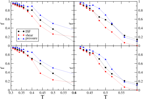
V.4 Tail-weight parameter $f$

Figure 10 shows the temperature dependence of the parameter $f$, the weight of the negative tail in the memory function relative to $K_{0}$ (with no cut-off included). As $T$ decreases, $f$ increases from a low value, approaching a value close to unity at the lowest temperatures. This increase accounts for that of the overall relaxation times $\tau_{\alpha}$ though the factor $1/(1-f)$. The value unity cannot be reached while remaining in equilibrium—because this implies a diverging relaxation time—unless the power-law behavior is cut off at the longest times. Thus there are two possibilities for the low-temperature behavior of $f$. The first is that it bends over and never reaches unity at finite temperature. In this case we can avoid including a cut-off, but the exact temperature dependence of $f$ determines that of $\tau_{\alpha}$, given that $\alpha$ seems to become temperature-independent at such temperatures. The second possibility is that $f$ becomes unity at a finite temperature, for example $T\sim$0.3 in 2D or $T\sim$0.4 in 3D. If this happens a cut-off must be included to keep $\tau_{\alpha}$ finite. When considering the full temperature range there does seem to be a bend over towards smaller slopes at lower temperatures, but the data in Fig. 10 are not clean enough to draw a firm conclusion about the limiting $T$-dependence of $f$.

V.5 Comparison with KWW fits, identification of common $\alpha$

Figure 11: (Color online) Comparison of $2-\alpha$ (determined using 3-parameter, unconstrained fits) with the stretching parameter $\beta_{KWW}$ in a fit to the stretched exponential for 2D (left) and 3D (right) simulations.. Open (black) symbols are values of $\beta_{KWW}$, taking values above 0.5, solids (red) symbols are values of $2-\alpha$, taking values below 0.5.

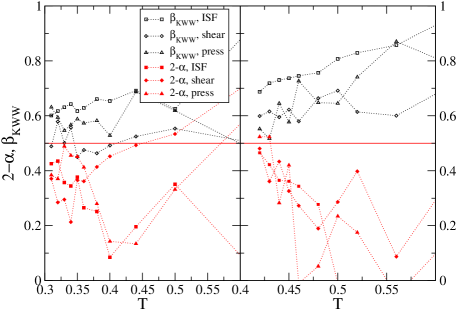
It is interesting to compare with a more common characterization of the shape, the stretching parameter $\beta_{KWW}$ in the KWW function. As explained in Sec. VI.2, this may be compared to $2-\alpha$, shown in Fig. 11. The values of $\beta_{KWW}$ decrease as $T$ decreases, while $2-\alpha$ increases. In a broad sense it seems that all are converging to a value around 0.5, but the degree of convergence for $\beta_{KWW}$ is much weaker. Considering the 3D data in particular, the values of $2-\alpha$ are within the range 0.47–0.52, while those of $\beta_{KWW}$ are spread over the range 0.55-0.7. The same trend can be seen, although less clearly, in the 2D data. It is possible that the $\beta_{KWW}$ values will converge at longer time scales, but the fact that $\alpha$ (or $2-\alpha$) seems to converge more rapidly to a common value suggests that this representation may be more physically meaningful. The value $\beta_{KWW}=$0.5, corresponding to $\alpha=$1.5, is interesting, because it has been argued theoretically and experimentally that this value is generic for structural “alpha” relaxation in viscous liquids, see Refs. Dyre, 2005b, a, 2006, 2007; Nielsen et al., 2008 and references therein.

Figure 12: (Color online) Results of a constrained 4-parameter fit of $F(q_{m},t)$ for all temperatures, where $\alpha$ is held fixed. Left panel shows data for 2D, right panel for 3D.

Figure 13: (Color online)Temperature dependence of $\tau_{s}$ (symbols + solid lines) and $\tau_{c}$ (symbols + dashed lines) for all correlation functions where $\alpha$ has been fixed at 1.58 (2D, left panels) and 1.5 (3D, right panels). While the 2D data does not fix $\tau_{c}$ very well (probably because simply it is larger relative to the relaxation time and therefore much more subject to noise in the tail), it seems plausible that a common value of $\tau_{c}$ for the three correlation functions could apply in 3D.

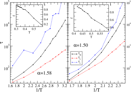
Given the apparent convergence to a common value of $\alpha$, and the hint in the 4-parameter fits to the ISF in 3D (lower-right panel of Fig. 9) that this parameter may in fact be temperature dependent, we have tried to fit the high quality ISF data with a common value of $\alpha$ over the whole temperature range, with the exponential cut-off included. The results are shown in Fig. 12. The common values of $\alpha$ that emerge from the fit are 1.58 for the 2D system and 1.50 for the 3D system. The quality of the “temperature-constrained” fits is is virtually indistinguishable by eye from that of the unconstrained 4-parameter fits (not shown). The latter, are of course, numerically superior (since they are unconstrained), but this seems to be mostly due to better matching of the noise in the tail. This result strengthens the case for $\alpha$ having a true value of 1.5 in 3D, independent of temperature. The other interesting feature of this constrained-$\alpha$ fit is that the temperature dependence of the time-scale $\tau_{c}$ of the exponential is much smoother, apparently tracking that of the relaxation time. What about the shear and pressure data? The data was of too low quality for an unconstrained four-parameter fit to work, but by fixing $\alpha$ to be equal to 1.5 we can include the exponential cut-off, making it effectively a three-parameter fit. The goodness of fit is consistently better than the original three-parameter fit (not shown), and now much smoother $\tau_{s}$ values, as well as $\tau_{c}$ values are available for shear and pressure. These are shown in Fig. 13. This works better for the 3D data than for the 2D data, which we suggest is due to the larger difference between $\tau_{\alpha}$ and $\tau_{c}$ in the latter case; the exponential cut-off has a significant effect only at longer times where the signal to noise ratio in the correlation function is smaller, and the fit thus gives erratic values.

In 3D the ratio $\tau_{c}/\tau_{\alpha}$ is in the range 2–3; in 2D the range is 8–9. Whether the cut-off time actually determines $\tau_{\alpha}$, or vice versa, or whether they determine each other in a self-consistent way, cannot be answered without a theoretical understanding and/or an explicit model for the relaxation. Nor do we know what may be the cause of the different ratios in 2D and 3D. To get a clearer picture more systems should be analyzed, and the possibility that $\tau_{c}$ is size dependent cannot be excluded.

V.6 Comparison of the fitted $K_{0}$ correspond with the actual short-time decay of the inherent quantities

A feature of our fitting procedure is that we leave the zero-time value of the correlation function as a fitting parameter, since the actual zero-time value of the true correlation function includes contributions from vibrational motion which rapidly decays. It is worth asking whether the value returned by the fit coincides with the value obtained by a careful determination of the inherent correlation function. Since we focus on time intervals of order $\Delta t\sim 20$, we can run relatively long simulations, and obtain good statistics for inherent quantities, by minimizing at similar intervals. For example minimizing once every 1000 time steps (100 times less frequently than before) corresponds to an interval $\Delta t=10$, and means that the simulation time is not dominated as much by the cost of minimizing. This was done in both the 2D and 3D systems for two temperatures: 0.34 and 0.40 for 2D and 0.44 and 0.52 for 3D. In addition runs with minimization every 100 time steps were carried out for 2D, $T=0.34$.

Figure 14: (Color online) Shear stress correlation functions and fits for 2D system at $T=0.34$. Main figure, comparison of true, inherent and fitted functions. The inherent function was based on minimization at intervals of 10 (1000 time steps); it has been rescaled to match the full correlation at $t=20$ (by a factor 0.97). The inset shows a zoom in of the inherent correlation function and the 4-parameter fit with $\alpha=1.58$ at short times. In this case the inherent correlation function was based on minimization every 1 unit (100 time steps); here the rescale factor is 0.99. The need to rescale simply reflects the sampling error in the variance ($t=0$ value); that of the autocovariance is almost the same (for relatively short lags), hence different sampling results in curves which are more or less proportional to each other. When comparing normalized correlation at, say $t=20$, the difference between minimization every 10 time steps (relatively short simulation times) and every 1000 time steps (relatively long simulation times) is of order 1%.

system	$T$	corr.	$\psi(\Delta t)_{I}$	$\psi(\Delta t)_{1.5}$	$\psi(\Delta t)_{3-p}$	$\psi(\Delta t)_{SE}$
2D	0.34	ISF	0.86	0.94	0.93	0.95
2D	0.34	shear	0.64	0.83	0.74	0.84
2D	0.34	press.	0.90	0.95	0.95	0.95
2D	0.40	ISF	0.72	0.83	0.71	0.84
2D	0.40	shear	0.46	0.56	0.60	0.54
2D	0.40	press	0.77	0.85	0.70	0.82
3D	0.44	ISF	0.94	0.97	0.97	0.98
3D	0.44	shear	0.78	0.91	0.90	0.89
3D	0.44	press.	0.91	0.94	0.93	0.96
3D	0.52	ISF	0.70	0.79	0.73	0.81
3D	0.52	shear	0.34	0.43	0.46	0.40
3D	0.52	press.	0.65	0.68	0.66	0.73

Table 1: Value of correlation functions (normalized to equal unity at time zero) at time $\Delta t=20$; comparison between actual inherent value (“I”) determined from the autocorrelation function of inherent quantities and values inferred from fitting the correlation function at longer times. Values for three fits are shown: (“1.5”) the fit with $\alpha$ fixed at be 1.5, including the exponential cut-off; (“$3-p$”) the 3-parameter fit with no cut-off; and (“SE”) the stretched exponential fit. The correlation at $\Delta t$ implied by the fits is higher than the actual correlation; alternatively put, the amount of decorrelation that takes place on the time scale $\Delta t$ is less than would be expected from the fits.

Table 1 shows values of the normalized correlation function after one time interval $\Delta t=20$, for two selected temperatures in each system, determined directly from the inherent state dynamics and inferred from different fits to the data for $t\geq\Delta t$. Although there are some exceptions (particularly for 2D, $T=0.40$), the trend is that the value of the normalized inherent correlation implied by the fits is higher than the actual value. For example for 2D at $T=0.34$, considering the intermediate scattering function, the actual correlation is 0.86, while the fits all imply a value between 0.93–0.94. Another way of putting this is that the amount of decorrelation that takes place between time zero and time $\Delta t$ is greater than is implied by the fits of the correlation at longer times (note that $\psi(\Delta t)=\psi_{1}=1-K_{0}$). This can be thought of as somewhat analogous to the extra relaxation associated with the vibrational motion which has been removed, but this is part of the inherent relaxation. Schrøder et al. also noticed a short-time component of the inherent structural relaxation (intermediate scattering function) which was not accounted for by stretched exponential fits.Schrøder et al. (2000) This was particularly noticeable at high temperatures and appeared to disappear in the activated regime. The comparison above suggests that this extra relaxation does not vanish, even at quite low temperatures. This discrepancy, between the very short-time relaxation and that for later times ($t>\Delta t$), presumably corresponds to the change of apparent power-law exponent in the memory function around this time scale (section IV.2). One could speculate that the existence of this extra component of the inherent relaxation could be associated with very small energy barriers, much smaller than the temperature. Such barriers would separate distinct inherent states, and thus “transitions” would show up in the inherent correlation functions, but these transitions would not be activated. The author has determined that the energy barriers in these systems are exponentially distributed, thus there are always some small barriers.Bailey (2009)

V.7 Wavenumber dependence of intermediate scattering function

Figure 15: (Color online) Wavenumber-dependent intermediate scattering function (symbols and dotted lines) and 4-parameter fits with $\alpha=1.5$ (solid lines), for 3D system, $T$=0.48. The inset shows the $q$-dependence of the tail-weight parameter $f$.

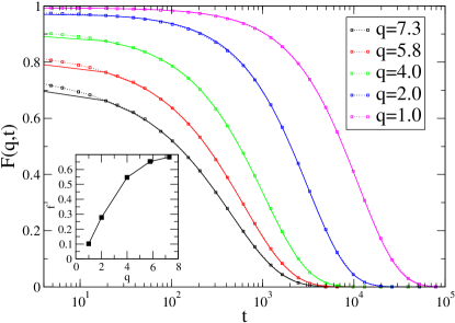
For simplicity, in studying the intermediate scattering above, we have restricted the analysis to a particular wavenumber, $q_{m}$, and to large particles. Given that a common value of the exponent $\alpha$ seems to be valid for the three correlation functions we have focused on so far, it makes sense to ask whether this applies for the intermediate scattering function at other $q$-values. In particular, what happens at low $q$, where we know that the relaxation becomes more exponential? Fig. 15 shows data and fits for 3D at $T=0.46$. Here 4-parameter fits with fixed $\alpha=1.5$ were used.

Figure 16: (Color online) Main figure, double-log plot of the $q-$dependence of the time-scales associated with the 4-parameter fit: the relaxation time $\tau_{\alpha}$, the inverse of short-time rate, $\tau_{s}$, and the exponential cut-off time $\tau_{c}$. A line proportional to $q^{-2}$ is shown as a guide to the eye. The $q$ values used are as in Fig. 15.

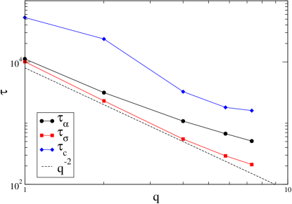
Figure 16 shows the $q$-dependence of the relaxation time $\tau_{\alpha}$, inverse of the short time rate, $\tau_{s}$ and the cut-off time of the memory function $\tau_{s}$. The inset shows the $q$-dependence of $f$. While the power-law exponent is fixed at 1.5 for all $q$-values, $f$ varies strongly, approaching zero at small $q$. This corresponds to relaxation that becomes exponential in this limit. Consistent with this, $\tau_{s}$ and $\tau_{\alpha}$ approach each other. $\tau_{c}$ seems to follow $\tau_{\alpha}$. In normal diffusion one expects the relaxation time to be proportional to $q^{-2}$, indicated by the dashed line. The relaxation time seems to approach this dependence in the low-$q$ limit (as is expected, given that diffusion should be normal at long length and time scales). More interesting is that $\tau_{s}$ seems to show an inverse square dependence over most of its range, corresponding to normal-diffusive behavior being observed at short times. This will be discussed below.

VI Discussion

VI.1 Generalized Langevin equations and continuous-time random walks

What does a negative inverse power-law memory function mean? One interpretation derives from the formalism of the generalized Langevin equation (GLE), which offers a framework for interpreting memory functions. The GLE for a dynamical variable $A(t)$ is a stochastic differential equation

$$\frac{dA}{dt}=-\int_{0}^{t}K(t-t^{\prime})A(t^{\prime})dt^{\prime}+F(t).$$ (17)

The first term on the right hand side involves an effective friction, non-local in time, where the memory kernel $K(t-t^{\prime})$ connects the friction at current time $t$ with the value of $A$ at a (previous) time $t^{\prime}$. The last term $F(t)$ is the so-called random force, or noise term. According to the second fluctuation-dissipation theorem, the memory kernel is the autocorrelation function of the noise, or

$$K(t)=\langle F(0)F(t)\rangle.$$ (18)

It may also be shown that this memory kernel $K(t)$ is the memory function associated with the autocorrelation of $A(t)$—the same memory function used in the analysis of this paper. Therefore one can interpret the obtained memory functions as the autocorrelation functions of the random force of the corresponding GLE. By “force” is meant the stochastic increment to the quantity $A$; in the original version of the Langevin equation $A$ was the velocity of a particle, whose change was indeed a force (divided by mass). Negative $K(t)$ for $t>0$ implies that the changes, which are presumably related to the so-called “flow-events” which define the long-time dynamics, are anti-correlated. The simplest interpretation of this would be forward-backward correlation of events—that is, an event is more likely to be the reverse of the previous one than to be something else. The parameter $f$ is then a direct measure of this anti-correlation. As it approaches unity, this tendency becomes so strong that the relaxation time diverges (see the next subsection).

An alternative interpretation involves uncorrelated events but with a non-exponential waiting-time distribution. This can be understood within the continuous-time random walk formalism of Montroll and Weiss.Montroll and Weiss (1965) The Montroll-Weiss equation relates the Laplace transform of $F(q,t)$ to the Laplace and Fourier transforms of the waiting-time and jump-size distributions, $\tilde{p}_{w}(s)$ and $\tilde{p}_{j}(k)$, respectively. It is straightforward to use it to derive a relation between the waiting-time distribution and the memory function. Skipping the details, this yields

$$\tilde{p}_{w}(s)=\frac{\tilde{K}(s)}{\tilde{K}(s)+s(1-\tilde{p}_{j}(k))}.$$ (19)

This relation can be considered a formal equivalence of the two pictures—anti-correlated random forces and non-exponential waiting-time distribution. The question of which picture is physically more relevant can only be determined by more detailed analysis of the dynamics in simulations. The existence of forward-backward correlations has indeed been noted by Heuer and coworkers (see Ref. Heuer, 2008 for a review of this work), but they argue that these are trivial, operating only on relatively short time scales. They have proposed a procedure for coarse-graining the dynamics by grouping the basins of attraction of inherent states together to form “meta-basins” (MBs). The definition of an MB is based on the requirement that once the system has escaped from an MB, it is unlikely to return there. They have shown that the dynamics on long time scales is essentially a random walk among MBs, but with non-trivial waiting-time distribution.Rubner and Heuer (2008) If we accept this interpretation, the memory function analysis presented here could be used as a way to find the waiting-time distribution from the correlation function. For example, in the $f\rightarrow 1$ limit with no cut-off (see next section) one finds that the waiting time distribution has a power-law tail with the exponent $\alpha$ as the memory function itself.

On the other hand, is it possible that the equivalence between the waiting time distribution point of view and the forward-backward point of view is in fact more than formal? The non-exponential distribution of waiting times could seen as a consequence of forward-backward correlations. The size of an MB is not a fixed property of the landscape,Doliwa and Heuer (2003) instead being defined in terms of dynamical behavior: a given MB can increase in size as temperature decreases, reflecting the increased tendency for returns (the system needs to get further away on average before its chance of escaping for good exceeds 50%). Correspondingly, the “anti-correlation tendency” $f$ increases towards unity; as long as it is less than unity, however, a diffusive regime is reached—the system will eventually forget where it started. In the “CTRW picture”, as long as the waiting-time distribution has a finite mean, upon sufficient coarse-graining it will become exponential and therefore the dynamics will be diffusive in the normal sense. The point of Heuer and co-workers is that there is a coarse-graining time scale at which events are uncorrelated but the waiting-time distribution is non-trivial (non-exponential). It is also true in the “GLE picture” involving anti-correlated events that, as long as $f<1$ or there is an exponential cut-off, a normal diffusive regime must also eventually be reached under coarse-graining in time. But it is not clear yet whether coarse-graining in the GLE picture can produce a dynamics that corresponds to the CTRW picture. This is a matter for future investigations.

VI.2 The $f=1$ limit: sub-diffusion

In this section we discuss briefly the limit $f\rightarrow 1$, in the case where there is no exponential cut-off. As mentioned, in this limit the relaxation time diverges, but the dynamics defined by this memory function are still meaningful, and have been studied in the context of anomalous diffusion, fractional Brownian motion and related processes. Metzler and Klafter (2000); Rangarajan and Ding (2003) Applications include protein dynamicsKneller and Hinsen (2004); Min et al. (2005) and dielectric response of glassy media. Goychuk (2007) A noise term in a GLE with this kind of correlation function is termed fractional Gaussian noise; when it acts on an unbound degree of freedom, the latter undergoes fractional Brownian motion. Correlation functions generally involve a function known as the Mittag-Leffler (ML) function: They behave at intermediate times like a stretched exponential, with stretching parameter $\beta_{KWW}=2-\alpha$, before switching to a power-law at long times, such that the integral is infinite. This is why it made sense to compare $2-\alpha$ with the fitted $\beta_{KWW}$ in Fig. 11.

There are two broad classes corresponding to positively or negatively correlated noise. When comparing to the literature on fractional diffusion and related processes it is important to realize that the Langevin equation is typically formulated with the dynamical variable $A(t)$ as the velocity of a particle. For a free particle, if the noise is fractional Gaussian with negative correlation, then the velocity autocorrelation function is an ML function. Its integral diverges, therefore the position dynamics is actually super-diffusive. Applications more typically involve sub-diffusive motion of a harmonically bound particle.Min et al. (2005) The noise acting on the velocity is positively correlated and it is the position autocorrelation function that decays as an ML function.

The memory function corresponding to this limit is $\tilde{K}(s)=s^{\alpha-1}$, which is clearly scale invariant: Rescaling, or coarse-graining in time produces the same dynamics. This corresponds to a fixed point in the renormalization group sense. For negatively correlated noise, the fixed point is unstable (see the chapter by Qian in Ref. Rangarajan and Ding, 2003)—if we are not quite in this limit, then rescaling will eventually takes us away from it and back to the normal diffusive regime, as discussed in the previous subsection. The results of the analysis presented in this paper could be therefore interpreted as saying that glassy dynamics approaches sub-diffusive dynamics with a particular exponent $\alpha$, which (in 3D) is very close to 1.5. As the limit $f=1$ is approached the relaxation becomes close to a Mittag-Leffler function, resembling a stretched exponential with $\beta_{KWW}=0.5$. As we have seen, even at the lowest temperatures, actually fitting with a stretched exponential yields a different exponent, so it is hard to see the convergence to 0.5, while this is clearer in the memory function based approach. The theoretical challenge is, of course, to understand where this exponent comes from, although there are models for viscous liquid dynamics which predict it (Refs. Dyre, 2005b, a, 2006, 2007; Nielsen et al., 2008 and references within).

Does this limit ever get reached? Although $f$ clearly approaches unity, it has not reached it yet at the temperatures simulated so far. Moreover, there is always an exponential cut-off in the memory function. Thus regardless of whether $f$ actually reaches unity or not, it will at some point be the exponential cut-off which will determine the relaxation time. Looking at Fig. 13, for example, suggests that this will happen around $T=0.40$ in 3D. Simple-minded linear or quadratic extrapolation of $f$ suggests this also. If we set $f=1$ for temperatures below say $T=0.40$ and assume that the exponential cut-off, $\tau_{c}$ is a fixed multiple of $\tau_{\alpha}$ (actually the ratio seems to increase), then one can make an extrapolation of $\tau_{\alpha}$, which gives a sharp crossover to an almost Arrhenius form (not shown). If $f$ approaches unity more smoothly, then the crossover will not be so abrupt, but in any case we predict that a change in the temperature dependence will occur around $T=0.40$.

VI.3 Short-time dynamics

The parameter $\tau_{s}=\Delta t/K_{0}$ is a measure of the dynamics at short times. By fixing the time scale, it measures how much activity happens in a given time, as opposed to standard measures of relaxation, which concern how much time is required for a given amount of relaxation to occur. For exponential relaxation there is no difference, for relatively small intervals (or long relaxation time $\tau_{\alpha}$): If the interval is $\Delta t$, then the amount of correlation at this time is

$$1-K_{0}=\exp(-\Delta t/\tau_{\alpha})\simeq 1-\Delta t/\tau_{\alpha},$$ (20)

which gives $\tau_{s}=\tau_{\alpha}$. Thus a difference between these two quantities is equivalent to non-exponential relaxation. When $\Delta t$ is much smaller than $\tau_{\alpha}$, the expected number of activated events that take place in a small volume in a time interval of this length is much smaller than unity, thus we cannot expect to see any correlation effects. We suggest therefore that $\tau_{s}$ is like a “bare” relaxation time, measuring the dynamics before correlation effects play a role. Recall (Fig. 14) that there is a noticeable amount of (inherent) relaxation in this time interval which is not accounted for by the fitted $\tau_{s}$. We assume this to be non-activated relaxation, and not relevant for what takes place at longer time scales (in this sense it resembles the vibrational part of the relaxation). The evidence supporting the idea of $\tau_{s}$ as a measure of the bare, uncorrelated relaxation rate is the near-Arrhenius temperature dependence (see Fig. 13), and the near $q^{-2}$ wavenumber dependence (Fig. 16) The use of a fixed, relatively short time interval to extract an apparent “underlying Arrhenius behavior” in viscous liquid dynamics was recently demonstrated by de Souza and Wales de Souza and Wales (2006a, b). They studied the diffusion constant determined by the mean squared displacement in a fixed time interval of 25 LJ units. They were also able to explicitly relate the deviations from exponential relaxation to anti-correlation of events in subsequent time windows. The present results are essentially equivalent, but obtained in the more general context of studying an arbitrary autocorrelation function.

VII Conclusion

We have presented a method for fitting the kind of slowly decaying autocorrelation functions typical of the dynamics of glass-forming liquids. An explicit functional form is postulated, not for the autocorrelation function, but for its associated memory function: a positive zero-time parameter $K_{0}$, and a negative inverse power law for non-zero time. An long-time exponential cut-off may optionally be included. This involves another parameter, although we have shown that good fits may be obtained by fixing the exponent to a common value, reducing the number of parameters per data set essentially to three. While it is possible to obtain the exact memory function from the autocorrelation function, it is not useful to fit the former directly. Rather we match the autocorrelation function by optimizing the parameters defining the memory function. Using a quite general functional form for $K(t)$ we noted a crossover from one apparent power-law to another at relatively short times, which allowed a simplification by considering data separated at times longer than the cross-over, namely the simple power-law form (with possible exponential cut-off). In particular we chose $\Delta t=20$ in Lennard-Jones units for all of the analysis. While the fits are about as good as fits with a stretched exponential, the parameters obtained have arguably greater physical significance than those of the latter. In particular the exponent $\alpha$ seems to be more or less independent of the relaxing quantity, and indeed of temperature (as long as the exponential cut-off is included), which is not the case for the stretching parameter $\beta_{KWW}$. Moreover the parameter $K_{0}$ may be interpreted as a short time rate; its temperature dependence is, interesting, significantly weaker than that of the alpha relaxation times for the different autocorrelation functions. As temperature decreases, the amplitude of the power tends to approach a limiting value associated with the mathematical description of anomalous diffusion/relaxation characterized mathematically by the Mittag-Leffler function. We hypothesize that this value is reached at finite temperature but the associated divergence of relaxation time is removed by the presence of an exponential cut-off. Including the latter in the fits for the self-intermediate scattering function allowed the identification of a third time scale, longer than the alpha time. It is hypothesized that the strong non-Arrhenius temperature dependence is due to a crossover from the time associated with the short-time rate to that associated with the long-time cut-off of the memory function, and that in particular at temperatures somewhat lower than those simulated, the non-Arrhenius behavior will weaken noticeably.

Appendix A Memory function fitting

Here we describe in a little more detail how we optimize the fit. We start by describing the procedure using the general fitting form which includes the piecewise linear function $L(t)$. Suppose first we have a correlation function based on inherent dynamics, so that there is no vibrational decay at short times, and in particular the $t=0$ value is known. Then we may normalize by the latter to get the normalized autocorrelation function $\psi(t)=\psi_{n}$ where $n=t/(\Delta t)$ $n$ is the integer corresponding to $t$. We write the fitting form as $K^{fit}_{n}(\{p_{a}\})$, where $p_{1},p_{2},\ldots$ are the parameters of the fitting form. The node values $L_{k}$ are not used directly as parameters; rather their logarithms are. This constrains them to be positive and minimizes numerical problems associated with the broad range of values that they turn out to have. For given values of the $\{p_{a}\}$, we can easily compute the associated correlation function $\psi^{fit}_{n}(\{p_{a}\})$ and then the objective function

$$F_{obj}(\{p_{a}\})=\sum_{n}\left(\psi(t)-\psi_{gen}(t,\{p_{a}\})\right)^{2}.$$ (21)

To minimize $F_{obj}$ we used the conjugate gradient technique,Press et al. (1987) calculating the gradient numerically.

For the main data analysis we switched to using simpler functional forms without the piecewise linear function. Also significant is that we used only the true dynamical correlation functions (as opposed to those of the inherent dynamics) which are more accurate and smooth; this removed the need to do expensive minimizations. By considering times at intervals of order 20, we could avoid the vibrational decay, except that now the correct initial value of correlation function had to be treated as an unknown parameter. Since this affects the normalization, it is important to handle this carefully. Suppose we have a non-normalized correlation function at discrete times, not including time zero: $C_{1},C_{2},C_{3},\ldots$. Since we are going to normalize anyway, we choose as the parameter not $C_{0}$, but the ratio $R_{01}\equiv C_{0}/C_{1}$. And since this is required be greater than unity, it is represented internally (i.e., within the fitting algorithm) in terms of a logarithm $\theta_{R}$: $R_{01}=1+\exp(\theta_{R})$, where $\theta_{R}$ is the actual parameter varied by the algorithm. Note that $R_{01}$ is directly related to $K_{0}$:

$$K_{0}=1-\psi_{1}=1-(C_{1}/C_{0})=1-1/R,$$ (22)

so that one may equivalently consider $K_{0}$ as the fitting parameter. An important technicality must be mentioned here. If the objective function is defined as above, there is a problem due to the fact that the normalization factor is now an adjustable parameter. This means that the objective function could be reduced by making $R_{01}$, and hence $C_{0}$, larger. This was found to be a problem for data sets from higher temperatures where the relaxation times were relatively short and therefore the data was not sufficient to constrain $R_{01}$ to reasonable values. The problem was solved by normalizing by the fixed quantity $C_{1}$ instead (but only for the purposes of defining the objective function). For $n>0$ (times greater than $\Delta t=20$) we used in some cases the single power law of Eq. 14. The tail-weight fraction $f$ is constrained to lie between 0 and 1 by expressing it internally as the $f=\arctan(f_{1})$ where $f_{1}$ is unconstrained. The exponent $\alpha$ was represented as itself because it tended to vary within a relatively small range (1.5–2.2), with no risk of assuming values which would cause numerical problems. In other cases an exponential cut-off factor was included, Eq. 16, which involves the timescale $\tau_{cut}$. Because this can vary over several orders of magnitude, to aid convergence it was expressed internally in terms of its logarithm, $\tau_{cut}=\exp(10\theta_{\tau})$, where the factor 10 was found to improve convergence (presumably by making the typical values and range of $\theta_{\tau}$ comparable to those of other parameters).

References

- Chaikin and Lubensky (1995) P. M. Chaikin and T. C. Lubensky, Principles of condensed matter physics (Cambridge University Press, 1995).
- Brawer (1985) S. Brawer, Relaxation in Viscous Liquids and Glasses (American Ceramic Society, 1985).
- Ediger et al. (1996) M. D. Ediger, C. A. Angell, and S. R. Nagel, J. Phys. Chem. 100, 13200 (1996).
- Boon and Yip (1980) J. P. Boon and S. Yip, Molecular Hydrodynamics (Dover, 1980).
- Kohlrausch (1854) R. Kohlrausch, Pogg. Ann. Phys. 91, 179 (1854).
- Williams and Watts (1970) G. Williams and D. C. Watts, Trans. Faraday Soc. 66, 80 (1970).
- Olsen et al. (2008) N. B. Olsen, T. Hecksher, K. Niss, and J. C. Dyre (2008), eprint arXiv:0811.0994v1.
- Szamel and Flenner (2006) G. Szamel and E. Flenner, Phys. Rev. E 73, 011504 (2006).
- Stariolo and Fabricius (2006) D. A. Stariolo and G. Fabricius, J. Chem. Phys. 125, 064505 (2006).
- Zwanzig (1961) R. Zwanzig, Lectures in Theoretical Physics (Interscience, NY, 1961), vol. 3, p. 135.
- Mori (1965) H. Mori, Prog. Theor. Phys. 34, 399 (1965).
- Stillinger (1995) F. H. Stillinger, Science 267, 1935 (1995).
- Schrøder et al. (2000) T. B. Schrøder, S. Sastry, J. C. Dyre, and S. C. Glotzer, J. Chem. Phys. 112, 9834 (2000).
- Liao and S.-H.Chen (2001) C. Y. Liao and S.-H.Chen, Phys. Rev. E 64, 031202 (2001).
- Wilf (1994) H. S. Wilf, Generatingfunctionology (Academic, 1994), 2nd ed.
- Kob and Andersen (1994) W. Kob and H. C. Andersen, Phys. Rev. Lett. 73, 1376 (1994).
- Stoltze (1997) P. Stoltze, Simulation Methods in Atomic Scale Materials Physics (Polyteknisk Forlag, Lyngby, Denmark, 1997).
- Press et al. (1987) W. H. Press, B. P. Flannery, S. A. Teukolsky, and W. T. Vetterling, Numerical Recipes in C: The Art of Scientific Computing (Cambridge University Press, 1987), 1st ed.
- Bailey et al. (2009) N. P. Bailey, T. B. Schrøder, and J. C. Dyre, Phys. Rev. Lett. 102, 1055701 (2009).
- Dyre (2005a) J. C. Dyre, Europhys. Lett. 71, 646 (2005a).
- Dyre (2005b) J. C. Dyre, Phys. Rev. E 72, 011501 (2005b).
- Dyre (2007) J. C. Dyre, Phys. Rev. E 76, 041508 (2007).
- Nielsen et al. (2008) A. I. Nielsen, T. Christensen, B. Jakobsen, K. Niss, N. B. Olsen, R. Richert, and J. C. Dyre (2008), eprint arXiv:0811.1116v1.
- Dyre (2006) J. C. Dyre, Phys. Rev. E 74, 021502 (2006).
- Bailey (2009) N. P. Bailey (2009), to be published.
- Montroll and Weiss (1965) E. W. Montroll and G. H. Weiss, J. Math. Phys. 6, 167 (1965).
- Heuer (2008) A. Heuer, J. Phys.: Condens. Matter 20, 373101 (2008).
- Rubner and Heuer (2008) O. Rubner and A. Heuer, Phys. Rev. E 78, 011504 (2008).
- Doliwa and Heuer (2003) B. Doliwa and A. Heuer, Phys. Rev. E 67, 031506 (2003).
- Rangarajan and Ding (2003) G. Rangarajan and M. Ding, eds., Processes with Long-Range Correlations (Springer, 2003).
- Metzler and Klafter (2000) R. Metzler and J. Klafter, Phys. Rep. 339, 1 (2000).
- Kneller and Hinsen (2004) G. R. Kneller and K. Hinsen, J. Chem. Phys. 121, 10278 (2004).
- Min et al. (2005) W. Min, G. Luo, B. J. Cherayil, S. C. Kou, and X. S. Xie, Phys. Rev. Lett. 94, 198302 (2005).
- Goychuk (2007) I. Goychuk, Phys. Rev. E 76, 040102 (2007).
- de Souza and Wales (2006a) V. K. de Souza and D. J. Wales, Phys. Rev. Lett. 96, 057802 (2006a).
- de Souza and Wales (2006b) V. K. de Souza and D. J. Wales, Phys. Rev. B 74, 134202 (2006b).