Collision of Multimode Dromions and a Firewall in the Two Component Long Wave Short Wave Resonance Interaction Equation

Abstract

In this paper, we investigate the two component long wave short wave resonance interaction (2CLSRI) equation and show that it admits the Painleve property. We then suitably exploit the recently developed truncated Painleve approach to generate exponentially localized solutions for the short wave components $S^{(1)}$ and $S^{(2)}$ while the long wave L admits line soliton only. The exponentially localized solutions driving the short waves $S^{(1)}$ and $S^{(2)}$ in the y direction are endowed with different energies (intensities) and are called ”multimode dromions”. We also observe that the multimode dromions suffer intramodal inelastic collision while the existence of a firewall across the modes prevents the switching of energy between the modes.

I Introduction

Recent investigations of the integrable coupled nonlinear Schrödinger equation, namely the celebrated Manakov model, and the observation of intensity redistribution in the collision of solitons [1-5] have clearly pointed out their potential usage in the field of optical communications and have virtually set in motion the process of designing an all optical computing machine. In particular, the vector solitons undergoing energy sharing collision identified in the coupled NLS equation turned out to be the key in the growing list of alternatives to the paradigm of soliton based chips, at least for specialized applications including quantum computing [6], DNA computing [7] and dynamics based computing based on chaos [8].

It is known that the identification of dromions [9,10] in the Davey-Stewartson equation which is a (2+1) dimensional generalization of the NLS equation has given the much needed impetus to the investigation of (2+1) dimensional integrable models. These dromions which are localized exponentially in all directions are essentially driven by certain lower dimensional arbitrary functions of space and time. In fact, such lower dimensional arbitrary functions of space and time have consolidated the concept of integrability of the associated dynamical systems in (2+1) dimensions besides being tailor made for the construction of various kinds of localized solutions. Reflecting on the flurry of activities taking place in the field of optical communication ever since the identification of shape changing collision of vector solitons in the coupled NLS equation and the rapid strides made in the field of (2+1) dimensional nonlinear partial differential equations (pdes) after the observation of dromions in the Davey-Stewartson I (DSI) equations, one would be tempted to look for the possibility of identifying the counterparts of vector solitons in (2+1) dimensions as well.

In fact, the recent derivation of the two component long wave short wave resonance interaction (2CLSRI) equation in the context of the interaction of nonlinear dispersive waves on three channels [11] has only fuelled the anticipation to look for such localized excitations. This is also further supported by the study of collision behaviour of plane solitons admitted by the 2CLSRI equation recently [12]. In this paper, we investigate 2CLSRI equation and confirm its Painleve property. We then suitably employ the recently developed truncated Painleve approach [13-16] and generate multimode dromions. It should be mentioned that this is the first time the existence of exponentially localized solutions has been reported in a vector (2+1) dimensional nonlinear pde. Finally, we also study the unusual interaction of multimode dromions.

We now consider the two component long wave short wave resonance interaction (2CLSRI) equation in the following form

$$i(S_{t}^{(1)}+S_{y}^{(1)})-S_{xx}^{(1)}+LS^{(1)}=0,$$ (1a)

$$i(S_{t}^{(2)}+S_{y}^{(2)})-S_{xx}^{(2)}+LS^{(2)}=0,$$ (1b)

$$L_{t}=2(|S^{(1)}|^{2}_{x}+|S^{(2)}|^{2}_{x}).$$ (1c)

The above equation is the two component analogue of the long wave short wave resonance interaction equation investigated recently [13]. In eq.(1), $S^{(1)}$ and $S^{(2)}$ represent short waves while L denotes a long wave. In particular, it explains the interaction of long interfacial wave (L) and a short surface wave (S) in a two layer fluid. This equation has been investigated recently and line solitons have been generated [11,12].

II Singularity Structure Analysis

We now rewrite the above equation by putting $S^{(1)}=p$, ${S^{(1)}}^{*}=q$, $S^{(2)}=r$, ${S^{(2)}}^{*}=s$ as

$$i(p_{t}+p_{y})-p_{xx}+Lp=0,$$ (2a)

$$-i(q_{t}+q_{y})-q_{xx}+Lq=0,$$ (2b)

$$i(r_{t}+r_{y})-r_{xx}+Lr=0,$$ (2c)

$$-i(s_{t}+s_{y})-s_{xx}+Ls=0,$$ (2d)

$$L_{t}=2(pq)_{x}+2(rs)_{x}.$$ (2e)

We now effect a local Laurent expansion of the variables $p$, $q$, $r$, $s$ and $L$ in the neighbourhood of a noncharacteristic singular manifold $\phi(x,y,t)=0$, $\phi_{x}\neq 0$, $\phi_{y}\neq 0$. Assuming the leading order of the solutions of eq. (2) to have the following form

$$p=p_{0}\phi^{\alpha},q=q_{0}\phi^{\beta},r=r_{0}\phi^{\gamma},s=s_{0}\phi^{\delta},L=L_{0}\phi^{m},$$ (3)

where $p_{0}$, $q_{0}$, $r_{0}$, $s_{0}$ and $L_{0}$ are analytic functions of ($x$, $y$, $t$) and $\alpha$, $\beta$, $\gamma$, $\delta$ and $m$ are integers to be determined, we now substitute (3) into (2) and balance the most dominant terms to obtain

$$\alpha=\beta=\gamma=\delta=-1,m=-2,$$ (4)

with the condition

$$p_{0}q_{0}+r_{0}s_{0}=\phi_{x}\phi_{t},L_{0}=2\phi_{x}^{2}.$$ (5)

Now, considering the generalized Laurent expansion of the solutions in the neighbourhood of the singular manifold

$$p=p_{0}\phi^{\alpha}+...+p_{j}\phi^{j+\alpha}+...,$$ (6a)

$$q=q_{0}\phi^{\beta}+...+q_{j}\phi^{j+\beta}+...,$$ (6b)

$$r=r_{0}\phi^{\gamma}+...+r_{j}\phi^{j+\gamma}+...,$$ (6c)

$$s=s_{0}\phi^{\delta}+...+s_{j}\phi^{j+\delta}+...,$$ (6d)

$$L=L_{0}\phi^{\omega}+...+L_{j}\phi^{j+\omega}+...,$$ (6e)

the resonances which are the powers at which arbitrary functions enter into (6) can be determined by substituting (6) into (2). Vanishing of the coefficients of ($\phi^{j-3}$,$\phi^{j-3}$,$\phi^{j-3}$,$\phi^{j-3}$,$\phi^{j-3}$) leads to the condition

$$\left(\begin{array}[]{ccccc}-j(j-3)\phi_{x}^{2}&0&0&0&p_{0}\\ 0&-j(j-3)\phi_{x}^{2}&0&0&q_{0}\\ 0&0&-j(j-3)\phi_{x}^{2}&0&r_{0}\\ 0&0&0&-j(j-3)\phi_{x}^{2}&s_{0}\\ 2(j-2)q_{0}\phi_{x}&2(j-2)p_{0}\phi_{x}&2(j-2)s_{0}\phi_{x}&2(j-2)r_{0}\phi_{x}&-(j-2)\phi_{t}\end{array}\right)\left(\begin{array}[]{c}p_{j}\\ q_{j}\\ r_{j}\\ s_{j}\\ L_{j}\end{array}\right)=0.$$ (7)

From equation (7), one gets the resonance values as

$$j=-1,\ 0,0,0,\ 2,\ 3,\ 3,\ 3,\ 4.$$ (8)

The resonance at $j$ = -1 naturally represents the arbitrariness of the manifold $\phi(x,y,t)=0$. In order to prove the existence of arbitrary functions at the other resonance values, we now substitute the full Laurent series

$$p=p_{0}\phi^{\alpha}+\sum_{j}p_{j}\phi^{j+\alpha},\quad q=q_{0}\phi^{\beta}+\sum_{j}q_{j}\phi^{j+\beta},\quad r=r_{0}\phi^{\gamma}+\sum_{j}r_{j}\phi^{j+\gamma},$$

$$s=s_{0}\phi^{\delta}+\sum_{j}s_{j}\phi^{j+\delta},\quad L=L_{0}\phi^{\omega}+\sum_{j}L_{j}\phi^{j+\omega}$$ (9)

into equation (2). Now, collecting the coefficients of ($\phi^{-3}$,$\phi^{-3}$,$\phi^{-3}$,$\phi^{-3}$,$\phi^{-3}$) and solving the resultant equation, we obtain equation (5), implying the existence of a resonance at $j=0,0,0$.
Similarly, collecting the coefficients of ($\phi^{-2}$,$\phi^{-2}$,$\phi^{-2}$, $\phi^{-2}$, $\phi^{-2}$) and solving the resultant equations by using the Kruskal’s ansatz, $\phi(x,y,t)=x+\psi(y,t)$, we get

$$p_{1}=\frac{1}{2}[ip_{0}(\psi_{t}+\psi_{y})-2p_{0x}],$$ (10a)

$$q_{1}=\frac{1}{2}[-iq_{0}(\psi_{t}+\psi_{y})-2q_{0x}],$$ (10b)

$$r_{1}=\frac{1}{2}[ir_{0}(\psi_{t}+\psi_{y})-2r_{0x}],$$ (10c)

$$s_{1}=\frac{1}{2}[-is_{0}(\psi_{t}+\psi_{y})-2s_{0x}],$$ (10d)

$$L_{1}=0.$$ (10e)

Collecting the coefficients of ($\phi^{-1}$,$\phi^{-1}$,$\phi^{-1}$,$\phi^{-1}$,$\phi^{-1}$), we have

$$i(p_{0t}+p_{0y})-p_{0xx}+L_{0}p_{2}+L_{1}p_{1}+L_{2}p_{0}=0,$$ (11a)

$$-i(q_{0t}+q_{0y})-q_{0xx}+L_{0}q_{2}+L_{1}q_{1}+L_{2}q_{0}=0,$$ (11b)

$$i(r_{0t}+r_{0y})-r_{0xx}+L_{0}r_{2}+L_{1}r_{1}+L_{2}r_{0}=0,$$ (11c)

$$-i(s_{0t}+s_{0y})-s_{0xx}+L_{0}s_{2}+L_{1}s_{1}+L_{2}s_{0}=0,$$ (11d)

$$L_{1t}=2[p_{0x}q_{1}+q_{1x}p_{0}+p_{1x}q_{0}+p_{1}q_{0x}]+2[r_{0x}s_{1}+r_{1x}s_{0}+s_{1x}r_{0}+r_{1}s_{0x}]=0.$$ (11e)

From (11a),(11b),(11c) and (11d), we can eliminate $L_{2}$ to obtain the following three equations for the four unknowns $p_{2}$, $q_{2}$, $r_{2}$ and $s_{2}$,

$$L_{0}(p_{0}q_{2}-q_{0}p_{2})-(p_{0}q_{0xx}-q_{0}p_{0xx})-i(p_{0}(q_{0t}+q_{0y})+q_{0}(p_{0t}+p_{0y}))=0,$$ (11f)

$$L_{0}(p_{0}r_{2}-r_{0}p_{2})-(p_{0}r_{0xx}-r_{0}p_{0xx})-i(-p_{0}(r_{0t}+r_{0y})+r_{0}(p_{0t}+p_{0y}))=0,$$ (11g)

$$L_{0}(p_{0}s_{2}-s_{0}p_{2})-(p_{0}s_{0xx}-s_{0}p_{0xx})-i(p_{0}(s_{0t}+s_{0y})+s_{0}(p_{0t}+p_{0y}))=0,$$ (11h)

which ensures that one of the functions $p_{2}$, $q_{2}$, $r_{2}$ or $s_{2}$ is arbitrary. Obviously $L_{2}$ itself can be obtained from any one of the four equations (11a), (11b), (11c) or (11d). Similarly, collecting the coefficients of ($\phi^{0}$,$\phi^{0}$,$\phi^{0}$,$\phi^{0}$,$\phi^{0}$), we have

$$i(p_{1t}+p_{2}\psi_{t})+i(p_{1y}+p_{2}\psi_{y})-(p_{1xx}+2p_{2x})+L_{2}p_{1}+L_{3}p_{0}=0,$$ (12a)

$$-i(q_{1t}+q_{2}\psi_{t})-i(q_{1y}+q_{2}\psi_{y})-(q_{1xx}+2q_{2x})+L_{2}q_{1}+L_{3}q_{0}=0,$$ (12b)

$$i(r_{1t}+r_{2}\psi_{t})+i(r_{1y}+r_{2}\psi_{y})-(r_{1xx}+2r_{2x})+L_{2}r_{1}+L_{3}r_{0}=0,$$ (12c)

$$-i(s_{1t}+s_{2}\psi_{t})-i(s_{1y}+s_{2}\psi_{y})-(s_{1xx}+2s_{2x})+L_{2}s_{1}+L_{3}s_{0}=0,$$ (12d)

$$L_{2t}+L_{3}\psi_{t}=2[p_{0x}q_{2}+(p_{1x}+p_{2})q_{1}+(p_{2x}+p_{3})q_{0}$$

$$+q_{0x}p_{2}+(q_{1x}+q_{2})p_{1}+(q_{2x}+q_{3})p_{0}]+$$

$$2[r_{0x}s_{2}+(r_{1x}+r_{2})s_{1}+(r_{2x}+r_{3})s_{0}$$

$$+s_{0x}r_{2}+(s_{1x}+s_{2})r_{1}+(s_{2x}+s_{3})r_{0}].$$ (12e)

Equations (12a), (12b), (12c) and (12d) can be solved for $L_{3}$ as

$$L_{3}=\frac{1}{p_{0}}(-i(p_{1t}+p_{2}\psi_{t})-i(p_{1y}+p_{2}\psi_{y})+(p_{1xx}+2p_{2x})-L_{2}p_{1}),$$ (12f)

$$L_{3}=\frac{1}{q_{0}}(i(q_{1t}+q_{2}\psi_{t})+i(q_{1y}+q_{2}\psi_{y})+(q_{1xx}+2q_{2x})-L_{2}q_{1}),$$ (12g)

$$L_{3}=\frac{1}{r_{0}}(-i(r_{1t}+r_{2}\psi_{t})-i(r_{1y}+r_{2}\psi_{y})+(r_{1xx}+2r_{2x})-L_{2}r_{1})$$ (12h)

$$L_{3}=\frac{1}{s_{0}}(i(s_{1t}+s_{2}\psi_{t})+i(s_{1y}+s_{2}\psi_{y})+(s_{1xx}+2s_{2x})-L_{2}s_{1}).$$ (12i)

Making use of eqns. (5), (10) and (11), we find that the right hand sides of eqs. (12f), (12g), (12h) and (12i) are equal. This implies that we are left with two equations for five unknowns. So, any three of the five coefficients $p_{3}$, $q_{3}$, $r_{3}$, $s_{3}$ or $L_{3}$ are arbitrary. Now, collecting the coefficients of ($\phi$, $\phi$, $\phi$, $\phi$, $\phi$), we have

$$i(p_{2t}+2p_{3}\psi_{t})+i(p_{2y}+2p_{3}\psi_{y})-(p_{2xx}+4p_{3x}+6p_{4})$$

$$+L_{0}p_{4}+L_{2}p_{2}+L_{3}p_{1}+L_{4}p_{0}=0,$$ (13a)

$$-i(q_{2t}+2q_{3}\psi_{t})-i(q_{2y}+2q_{3}\psi_{y})-(q_{2xx}+4q_{3x}+6q_{4})$$

$$+L_{0}q_{4}+L_{2}q_{2}+L_{3}q_{1}+L_{4}q_{0}=0,$$ (13b)

$$i(r_{2t}+2r_{3}\psi_{t})+i(r_{2y}+2r_{3}\psi_{y})-(r_{2xx}+4r_{3x}+6r_{4})$$

$$+L_{0}r_{4}+L_{2}r_{2}+L_{3}r_{1}+L_{4}r_{0}=0,$$ (13c)

$$-i(s_{2t}+2s_{3}\psi_{t})-i(s_{2y}+2s_{3}\psi_{y})-(s_{2xx}+4s_{3x}+6s_{4})$$

$$+L_{0}s_{4}+L_{2}s_{2}+L_{3}s_{1}+L_{4}s_{0}=0,$$ (13d)

$$L_{3t}+2L_{4}\psi_{t}=2[p_{0x}q_{3}-p_{0}q_{4}+(p_{1x}+p_{2})q_{2}$$

$$+(p_{2x}+2p_{3})q_{1}+(p_{3x}+3p_{4})q_{0}+q_{0x}p_{3}-q_{0}p_{4}$$

$$+(q_{1x}+q_{2})p_{2}+(q_{2x}+2q_{3})p_{1}+(q_{3x}+3q_{4})p_{0}]+$$

$$2[r_{0x}s_{3}-r_{0}s_{4}+(r_{1x}+r_{2})s_{2}+(r_{2x}+2r_{3})s_{1}+$$

$$(r_{3x}+3r_{4})s_{0}+s_{0x}r_{3}-s_{0}r_{4}$$

$$+(s_{1x}+s_{2})r_{2}+(s_{2x}+2s_{3})r_{1}+(s_{3x}+3s_{4})r_{0}].$$ (13e)

By multiplying (13a) by $q_{0}$, (13b) by $p_{0}$, (13c) by $s_{0}$, (13d) by $r_{0}$ and adding the resultant equation, we obtain an equation which is same as (13e). This means that we have only four determining equations for five unknowns. So, any one of the five functions $p_{4}$, $q_{4}$, $r_{4}$, $s_{4}$ or $L_{4}$ is arbitrary. One can proceed further to determine all other coefficients of the Laurent expansions (9) without the introduction of any movable critical manifold. Thus, the 2CLSRI equation indeed satisfies the Painlevé property.

III Truncated Painleve Approach and Localized Solutions

To generate the solutions of 2CLSRI equation, we now suitably exploit the results of the leading order behaviour by employing the truncated Painlevé approach. Truncating the Laurent series of the solutions of eq. (2) at the constant level term, one obtains following the Bäcklund transformation

$$p=\frac{p_{0}}{\phi}+p_{1},\quad q=\frac{q_{0}}{\phi}+q_{1},\quad r=\frac{r_{0}}{\phi}+r_{1},\quad s=\frac{s_{0}}{\phi}+s_{1},\quad$$

$$L=\frac{L_{0}}{\phi^{2}}+\frac{L_{1}}{\phi}+L_{2}.$$ (14)

Assuming the following seed solution

$$p_{1}=q_{1}=r_{1}=s_{1}=0,\quad L_{2}=L_{2}(x,y),$$ (15)

we now substitute (14) with the above seed solution (15) into equations (2) and obtain (5) by collecting the coefficients of $(\phi^{-3},\phi^{-3},\phi^{-3},\phi^{-3},\phi^{-3})$. Gathering the coefficients of $(\phi^{-2},\phi^{-2},\phi^{-2},\phi^{-2},\phi^{-2})$, we have the following system of equations

$$-ip_{0}\phi_{t}-ip_{0}\phi_{y}+2p_{0x}\phi_{x}+p_{0}\phi_{xx}+L_{1}p_{0}=0,$$ (16a)

$$iq_{0}\phi_{t}+iq_{0}\phi_{y}+2q_{0x}\phi_{x}+q_{0}\phi_{xx}+L_{1}q_{0}=0,$$ (16b)

$$-ir_{0}\phi_{t}-ir_{0}\phi_{y}+2r_{0x}\phi_{x}+r_{0}\phi_{xx}+L_{1}r_{0}=0,$$ (16c)

$$is_{0}\phi_{t}+is_{0}\phi_{y}+2s_{0x}\phi_{x}+s_{0}\phi_{xx}+L_{1}s_{0}=0,$$ (16d)

$$L_{0t}-L_{1}\phi_{t}=2(p_{0}q_{0}+r_{0}s_{0})_{x}.$$ (16e)

From equation (16e), we have

$$L_{1}=2\frac{(\phi_{x}\phi_{tx}-\phi_{xx}\phi_{t})}{\phi_{t}}.$$ (17)

Using (17) in (16a-16d), the variables $p_{0}$, $q_{0}$, $r_{0}$ and $s_{0}$ can be solved as

$$p_{0}=F_{1}(y,t)\mbox{exp}\bigg{[}{\frac{1}{2}\int\frac{i(\phi_{t}+\phi_{y})+\phi_{xx}-\frac{2\phi_{x}\phi_{tx}}{\phi_{t}}}{\phi_{x}}{\rm d}x}\bigg{]},$$

(18a)

$$q_{0}=F_{1}(y,t)\mbox{exp}\bigg{[}{\frac{1}{2}\int\frac{-i(\phi_{t}+\phi_{y})+\phi_{xx}-\frac{2\phi_{x}\phi_{tx}}{\phi_{t}}}{\phi_{x}}{\rm d}x}\bigg{]},$$

(18b)

$$r_{0}=F_{2}(y,t)\mbox{exp}\bigg{[}{\frac{1}{2}\int\frac{i(\phi_{t}+\phi_{y})+\phi_{xx}-\frac{2\phi_{x}\phi_{tx}}{\phi_{t}}}{\phi_{x}}{\rm d}x}\bigg{]},$$

(18c)

$$s_{0}=F_{2}(y,t)\mbox{exp}\bigg{[}{\frac{1}{2}\int\frac{-i(\phi_{t}+\phi_{y})+\phi_{xx}-\frac{2\phi_{x}\phi_{tx}}{\phi_{t}}}{\phi_{x}}{\rm d}x}\bigg{]},$$

where $F_{1}(y,t)$ and $F_{2}(y,t)$ are lower dimensional arbitrary functions of $y$ and $t$.

Substituting (18) in (5), we obtain the condition

$$F_{2}(t-y)^{2}=\phi_{t}-F_{1}(t-y)^{2}.$$ (19)

Again, collecting the coefficients of $(\phi^{-1},\phi^{-1},\phi^{-1},\phi^{-1},\phi^{-1})$, we have

$$ip_{0t}+ip_{0y}-p_{0xx}+L_{2}p_{0}=0,$$ (20a)

$$-iq_{0t}-iq_{0y}-q_{0xx}+L_{2}q_{0}=0,$$ (20b)

$$ir_{0t}+ir_{0y}-r_{0xx}+L_{2}r_{0}=0,$$ (20c)

$$-is_{0t}-is_{0y}-s_{0xx}+L_{2}s_{0}=0,$$ (20d)

$$L_{1t}=0.$$ (20e)

Making use of (17), we rewrite (20e) in the following trilinear form

$$\phi_{t}^{2}\phi_{xxt}-\phi_{x}\phi_{tx}\phi_{tt}+\phi_{xt}^{2}\phi_{t}+\phi_{x}\phi_{ttx}\phi_{t}=0.$$ (21)

The above trilinear equation ensures that the arbitrary manifold $\phi(x,y,t)$ should be partitioned as

$$\phi=\phi_{1}(x,y)+\phi_{2}(y,t),$$ (22)

where $\phi_{1}(x,y)$ and $\phi_{2}(y,t)$ are arbitrary functions in the indicated variables. Making use of (22) in eqs. (18a) and (18b), one can show that eqs. (20a-20d) are consistent provided the submanifold $\phi_{2}(y,t)$ can be split as

$$\phi_{2}(y,t)=\phi_{21}(y)+\phi_{22}(t-y),$$ (23)

Again, collecting the coefficients of $(\phi^{0},\phi^{0},\phi^{0},\phi^{0},\phi^{0})$, we have only one equation

$$L_{2t}=0.$$ (24)

Making use of (20a) for $L_{2}$, (24) reduces to the form

$$(F_{1tt}+F_{1ty})F_{1}+(F_{1t}+F_{1y})F_{1t}=0.$$ (25)

Equation (25) can be solved to obtain the form for $F_{1}(y,t)$ as

$$F_{1}(y,t)=F_{1}(t-y).$$ (26)

Thus, the solutions of 2CLSRI can be written as

$$S^{(1)}(x,y,t) = \frac{F_{1}(t-y)\sqrt{\phi_{1x}}e^{\int\frac{1}{2}\frac{i(\phi_{1y}+\phi_{21,y})}{\phi_{1x}}{\rm d}x}}{(\phi_{1}(x,y)+\phi_{21}(y)+\phi_{22}(t-y))},$$

$$S^{(2)}(x,y,t) = \frac{\sqrt{(\phi_{22,t}-F_{1}(t-y)^{2})\phi_{1x}}e^{\int\frac{1}{2}\frac{i(\phi_{1y}+\phi_{21,y})}{\phi_{1x}}{\rm d}x}}{(\phi_{1}(x,y)+\phi_{21}(y)+\phi_{22}(t-y))},$$

$$L = \frac{2\phi_{1x}^{2}}{(\phi_{1}(x,y)+\phi_{21}(y)+\phi_{22}(t-y))^{2}}$$ (28)

$$- \frac{2\phi_{1xx}}{(\phi_{1}(x,y)+\phi_{21}(y)+\phi_{22}(t-y))}+L_{2},$$

where

$$L_{2} = \int\frac{1}{2}\bigg{(}\frac{(\phi_{1yy}+\phi_{21,yy})-i\phi_{1xxy}}{\phi_{1x}}-$$

$$\frac{(\phi_{1y}+\phi_{21,y})-i\phi_{1xx}}{\phi_{1x}^{2}}\phi_{1xy}\bigg{)}dx$$ (29)

$$+ \frac{1}{2}\frac{i\phi_{1xy}+\phi_{1xxx}}{\phi_{1x}}-\frac{1}{4}\frac{(\phi_{1y}+\phi_{21,y})^{2}+\phi_{1xx}^{2}}{\phi_{1x}^{2}}.$$

Thus, by choosing the arbitrary functions $F_{1}(t-y)$, $\phi_{1}{(x,y)}$, $\phi_{21}(y)$ and $\phi_{22}(t-y)$ suitably, one can generate various kinds of localized solutions for the short waves $S^{(1)}$ and $S^{(2)}$ while the longwave L does not support completely localized solutions. From (27a) and (27b), it is also obvious that the two physical fields $S^{(1)}$ and $S^{(2)}$ have the same form except that their amplitudes are different and are driven by arbitrary functions $F_{1}(t-y)$ and $\sqrt{\phi_{22,t}-F_{1}(t-y)^{2}}$, respectively. It is also obvious that the 2CLSRI equation possesses an extra arbitrary function of space and time in comparison with its scalar counterpart [13].

IV Dromion solutions and their Interactions

Now we choose specific forms of the arbitrary functions in (28) and (29) and obtain explicit exponentially localized dromion solutions and study their interactions. To generate a (1,1) dromion for the modes $S^{(1)}$ and $S^{(2)}$, we choose the lower dimensional arbitrary functions of space and time, for example, as

$$F_{1}(t-y)=a_{1}sech(d_{1}(t-y)+e_{1})+g_{1}$$

$$\phi_{1}(x,y)=a_{2}tanh(b_{2}x+c_{2}y+e_{2})+g_{2}$$ (30)

$$\phi_{21}(y)=g_{3},\phi_{22}(t-y)=a_{4}tanh(d_{4}(t-y)+e_{4})+g_{4}$$

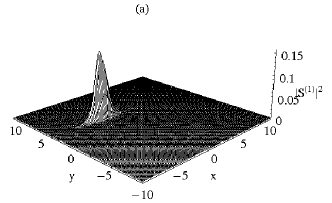
Figure 1: Intensity profile of the one dromion solution for (a) the first mode, (b) the second mode, (c) line soliton for the long wave component L at t=3.

Then, the corresponding exponentially localized solutions for $|S^{(1)}|^{2}$ and $|S^{(2)}|^{2}$ can be written as

$$|S^{(1)}|^{2}=\frac{\begin{array}[]{l}(a_{1}\sec h(d_{1}(t-y)+e_{1})+g_{1})^{2}{a_{2}b_{2}\sec h(b_{2}x+c_{2}y+e_{2})^{2}}\\ \end{array}}{{(a_{2}\tanh(b_{2}x+c_{2}y+e_{2})+g_{2}+g_{3}+a_{4}\tanh(d_{4}(t-y)+e_{4})+g_{4})^{2}}},$$ (32)

$$|S^{(2)}|^{2}=\frac{\begin{array}[]{l}\begin{array}[]{l}\left[a_{4}d_{4}\sec h(d_{4}(t-y)+e_{4})^{2}-(a_{1}\sec h(d_{1}(t-y)+e_{1})+g_{1})^{2}\right]\times\\ a_{2}b_{2}\sec h(b_{2}x+c_{2}y+e_{2})^{2}\\ \end{array}\\ \end{array}}{{(a_{2}\tanh(b_{2}x+c_{2}y+e_{2})+g_{2}+g_{3}+a_{4}\tanh(d_{4}(t-y)+e_{4})+g_{4}}}.$$ (36)

The variable $L$ takes the form

$$L = \frac{2a_{2}^{2}\sec h(b_{2}+c_{2}y+e_{2})^{4}}{(a_{2}\tanh(b_{2}x+c_{2}y+e_{2})+g_{2}+g_{3}+a_{4}\tanh(d_{4}(t-y)+e_{4})+g_{4})^{2}}$$ (37)

$$-\frac{4a_{2}b_{2}^{2}\sec h(b_{2}+c_{2}y+e_{2})^{2}\tanh(b_{2}+c_{2}y+e_{2})}{(a_{2}\tanh(b_{2}x+c_{2}y+e_{2})+g_{2}+g_{3}+a_{4}\tanh(d_{4}(t-y)+e_{4})+g_{4})}$$

$$-\frac{1}{4}\frac{c_{2}^{2}}{b_{2}^{2}}+b_{2}^{2}$$

A plot of the one dromion solution for the modes $S^{(1)}$ and $S^{(2)}$ for the following parametric choice, $a_{1}=1;a_{2}=a_{4}=0.6;b_{2}=1;c_{2}=1;d_{1}=d_{4}=4;e_{1}=e_{2}=e_{4}=0;g_{1}=g_{2}=g_{4}=0;g_{3}=3(a_{4}d_{4}>a_{1}^{2})$ is shown in figs. 1(a) and 1(b). From the figures, it is clear that the dromions for the modes $S^{(1)}$ and $S^{(2)}$ moving in the y-direction have different amplitudes and the amplitude of the dromions and hence the energy in a given mode depends on the parameter $a_{1}$. We call such exponentially localized solutions driving $S^{(1)}$ and $S^{(2)}$ as ”multimode dromions”. Further, the above choice of lower dimensional arbitrary functions of space and time given by eq. (30) yields a line soliton for the long wave L as shown in fig. 1(c).

To generate a $(2,1)$-dromion for $S^{(1)}$ and $S^{(2)}$, we choose

$$F_{1} =a_{1}sech(d_{1}(t-y)+e_{1})+g_{1}$$

$$\phi_{1} =a_{2}tanh(b_{2}x+c_{2}y+e_{2})+$$

$$a_{3}tanh(b_{3}x+c_{3}y+e_{3})+g_{2}$$ (38)

$$\phi_{21} =g_{3},\phi_{22}=a_{4}tanh(d_{4}(t-y)+e_{4})+g_{4}$$

so that the explicit solution can be written as

$$|S^{(1)}|^{2}=\frac{\begin{array}[]{l}(a_{1}\sec h(d_{1}(t-y)+e_{1})+g_{1})^{2}\begin{array}[]{l}[a_{2}b_{2}\sec h(b_{2}x+c_{2}y+e_{2})^{2}\\ +a_{3}b_{3}\sec h(b_{3}x+c_{3}y+e_{3})^{2}]\\ \end{array}\end{array}}{\begin{array}[]{l}[a_{2}\tanh(b_{2}x+c_{2}y+e_{2})+a_{3}\tanh(b_{3}x+c_{3}y+e_{3})+g_{2}+g_{3}+\\ a_{4}\tanh(d_{4}(t-y)+e_{4})+g_{4}]^{2}\\ \end{array}},$$ (44)

$$|S^{(2)}|^{2}=\frac{\begin{array}[]{l}\begin{array}[]{l}\left[a_{4}d_{4}\sec h(d_{4}(t-y)+e_{4})^{2}-(a_{1}\sec h(d_{1}(t-y)+e_{1})+g_{1})^{2}\right]\times\\ \left[a_{2}b_{2}\sec h(b_{2}x+c_{2}y+e_{2})^{2}+a_{3}b_{3}\sec h(b_{3}x+c_{3}y+e_{3})^{2}\right]\\ \end{array}\end{array}}{\begin{array}[]{l}[a_{2}\tanh(b_{2}x+c_{2}y+e_{2})+a_{3}\tanh(b_{3}x+c_{3}y+e_{3})+g_{2}+g_{3}+\\ a_{4}\tanh(d_{4}(t-y)+e_{4})+g_{4}]^{2}\\ \end{array}}.$$ (50)

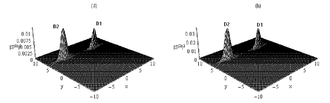
The plot of the (2,1) dromion solution for the modes $S^{(1)}$ and $S^{(2)}$ for the following parametric choice $a_{1}=1;a_{2}=1;a_{3}=1;a_{4}=1;b_{2}=b_{3}=1;c_{2}=1;c_{3}=-1;d_{1}=d_{4}=4;e_{1}=0;e_{2}=e_{3}=0;e_{4}=0;g_{1}=g_{2}=g_{4}=0;g_{3}=10(a_{4}d_{4}>a_{1}^{2})$ at t=-6, -4, -1, 5 is shown in figs. (2a-2h).

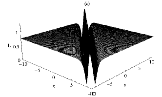
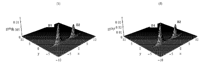
Figure 2: Intensity profiles of the two dromion solution for the first mode (4a-4d) and second mode (4e-4h) at t = -6.0, -4.0, -1.0, 5.0.

From the interaction of the dromions for the modes $S^{(1)}$ and $S^{(2)}$ shown in figs. (2a-2h), one observes that the two exponentially localized solutions with initial intensities $D_{1}$ and $D_{2}$ ($D_{1}>D_{2}$) move along the diagonals in the (x-y) plane and exchange their intensities (energies) among themselves after interaction ($D_{1}<D_{2}$) thereby undergoing intramodal inelastic collision. It is also interesting to note that there is no exchange of energy between the two constituent modes and the energy contained in a given mode remains a constant.

It should be mentioned that the choice of the lower dimensional arbitrary functions of space and time $F_{1}(t-y)$, $\phi_{1}(x,y)$, $\phi_{2}(y)$ and $\phi_{22}(t-y)$ determine the nature of the solutions admitted by 2CLSRI equation and their collision dynamics. For the choice of arbitrary functions given by eq.(30), one observes that the short waves are driven by exponentially localized solutions (dromions) and the energy contained in the first mode $S^{(1)}$ depends on $F_{1}(t-y)^{2}$ while for the second mode $S^{(2)}$, it is governed by $(\phi_{22,t}-F_{1}(t-y)^{2})$. For the choice given by eq.(30) (with the parameters as in fig.4), the amplitude (energy) of the first mode $S^{(1)}$ is governed by the one dimensional soliton $sech^{2}4(t-y)$ while for the second mode $S^{(2)}$, it depends on the soliton $3sech^{2}4(t-y)$. Thus, the choice given by eq. (30) launches two different energies in the modes $S^{(1)}$ and $S^{(2)}$ governed by the one dimensional solitons $sech^{2}4(t-y)$ and $3sech^{2}4(t-y)$, respectively, and since the amplitude (energy) of the solitons does not change during evolution, the energy contained in a mode remains a constant. Quantitatively, this is governed by the condition

$$\frac{|S^{(1)}|^{2}}{|S^{(2)}|^{2}}=\frac{F_{1}^{2}}{\phi_{22,t}-F_{1}^{2}}\quad\overrightarrow{t\rightarrow\pm\infty}\quad\frac{g_{1}^{2}}{g_{4}^{2}-g_{1}^{2}}=\rm{constant}$$ (51)

The above condition explains the existence of a firewall across the modes. This prohibition of energy across the modes by virtue of the existence of a firewall is valid only for the choice given by eq.(30), particularly if the short waves are to be driven by dromions. This behaviour in a vector (2+1) dimensional nonlinear pde is in sharp contrast to the Manakov model, a vector (1+1) nonlinear Schrodinger equation wherein the energy associated with the one dimensional solitons keeps flowing from one mode to the other. It should be mentioned that we report for the first time the identification of exponentially localized solutions in a vector (2+1) dimensional nonlinear pde and their collision dynamics.

From eqns. (27a) and (27b), one also observes that the sum of the squares of the short waves $S^{(1)}$ and $S^{(2)}$ obeys the following equation

$$|S^{(1)}|^{2}+|S^{(2)}|^{2}=\frac{\phi_{22,t}\phi_{1x}}{(\phi_{1}(x,y)+\phi_{21}(y)+\phi_{22}(t-y))^{2}}=S^{(1,2)}$$ (52)

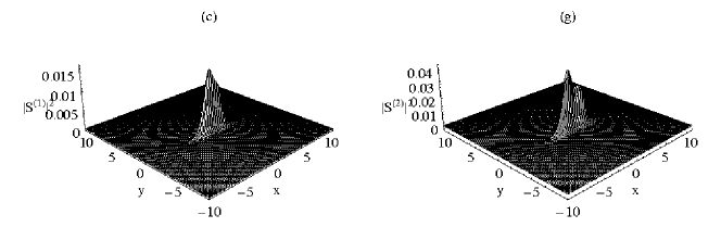
Figure 3: Time evolution of the composite mode $S^{(1,2)}$ at t= $-$6.0, 5.0

where we call $S^{(1,2)}$ as the ”composite mode”. Thus, we find that the composite mode $S^{(1,2)}$ is again driven by a two dromion solution (shown in figs.3((a),(b)) at t=$-$6, 5). The intensity of the solution for the composite mode $S^{(1,2)}$ is the sum of the constituent modes $S^{(1)}$ and $S^{(2)}$ at every instant of time and one also observes a similar inelastic collision in the composite mode $S^{(1,2)}$.

V Conclusion

In this paper, we have investigated the two component LSRI equation and shown that it admits Painleve property. We have then suitably exploited the truncated Painleve approach and generated multimode dromions for the short waves $S^{(1)}$ and $S^{(2)}$. The collision dynamics of multimode dromions generated in the paper indicates that they suffer intramodal inelastic collision while the existence of a firewall prevents the flow of energy from one mode to the other. It would be interesting to investigate the n-component LSRI equation from the perspective of localized solutions and their interaction.

Acknowledgements: RR wishes to acknowledge the financial assistance received from DST and UGC in the form of major and minor research projects. She also wishes to thank Indian National Science Academy (INSA) and Royal Society of London for sponsoring her visit to Glasgow under the bilateral exchange programme. The work of ML forms part of a Department of Science and Technology, Govt. of India research project and is also supported by a DST Ramanna Fellowship.

VI References