Europhysics Letters, 85 (2009) 49002
     
Transitional dynamics of the solar convection zone

Abstract

Solar activity is studied using a cluster analysis of the time-fluctuations of sunspot number. In the historic period (1850-1932) the cluster exponent $\alpha\simeq 0.37$ (strong clustering) for the high activity components of the solar cycles. In the modern period (last seven solar cycles: 1933-2007) the cluster exponent was $\alpha\simeq 0.50$ (random, white noise-like). Comparing these results with the corresponding data from laboratory experiments on convection it is shown, that in the historic period emergence of sunspots in the solar photosphere was dominated by turbulent photospheric convection. In the modern period, this domination was broken by a new more active dynamics of the inner layers of the convection zone. Cluster properties of the solar wind magnetic field and the aa-geomagnetic-index also support this result. Long-range chaotic dynamics in the solar activity is briefly discussed.

1 Introduction

The sunspot number is the main direct and reliable source of information about the solar dynamics for a historic period. In a recent paper [1], for instance, results of a reconstruction (based on radiocarbon concentrations, see also [2]) of the sunspot number were presented for the past 11,400 years. Analysis of this reconstruction showed an exceptional level of solar activity during the past seven solar cycles (1933-2007).

Figure 1: Daily sunspot number (SSN) vs time [12]. The dashed straight line separates between historic and modern periods.

Sunspots appear as the visible counterparts of magnetic flux tubes in the convective zone of the sun. Since a strong magnetic field is considered as a primary phenomenon that controls generation of the sunspots the crucial question is: Where has the magnetic field itself been generated? The location of the solar dynamo is the subject of vigorous discussions in recent years. A general consensus had been developed to consider the shear layer at the bottom of the convection zone as the main source of the solar magnetic field [3] (see, for a recent review [4]). In recent years, however, the existence of a prominent radial shear layer near the top of the convection zone has become rather obvious and the problem again became actual. The presence of large-scale meandering flow fields (like jet streams), banded zonal flows and evolving meridional circulations together with intensive multiscale turbulence shows that the near surface layer is a very complex system, which can significantly affect the processes of the magnetic field and the sunspots generation. There could be two sources for the poloidal magnetic field: one near the bottom of the convection zone (or just below it [3]), another one resulting from an active-region tilt near the surface of the convection zone. For the recently renewed Babcock-Leighton [5],[6] solar dynamo scenario, for instance, a combination of the sources was assumed for predicting future solar activity levels [7], [8]. In this scenario the surface generated poloidal magnetic field is carried to the bottom of the convection zone by turbulent diffusion or by the meridional circulation. The toroidal magnetic field is produced from this poloidal field by differential rotation in the bottom shear layer. Destabilization and emergence of the toroidal fields (in the form of curved tubes) due to magnetic buoyancy can be considered as a source of the pairs of sunspots of opposite polarity. The turbulent convection in the convection zone and, especially, in the near-surface layer captures the magnetic flux tubes and either disperses or pulls them trough the surface to become sunspots.

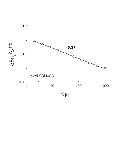
Figure 2: The standard deviation for $\delta n_{\tau}$ vs $\tau$ for the level SSN=85 (historic period) in log-log scales. The straight line (the best fit) indicates the scaling law Eq. (1).

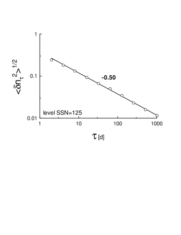
Figure 3: The standard deviation for $\delta n_{\tau}$ vs $\tau$ for the level SSN=125 (modern period) in log-log scales. The straight line (the best fit) indicates the scaling law Eq. (1).

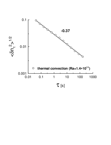
Figure 4: The standard deviation for $\delta n_{\tau}$ vs $\tau$ for the temperature fluctuations in the Rayleigh-Bernard convection laboratory experiment with $Ra=1.4\times 10^{11}$ [14]. The straight line indicates the scaling law Eq. (1).

The magnetic field plays a passive role in the photosphere and does not participate significantly in the turbulent photospheric energy transfer. On the other hand, the very complex and turbulent near-surface layer (including photosphere) can significantly affect the process of emergence of sunspot. The similarity of light elements properties in the spot umbra and granulation is one of the indication of such phenomena.

The paper reports a direct relation between the fluctuations in sunspot number and the temperature of turbulent convection in the photosphere for the historic period. This relation allows for certain conclusions about the generation mechanisms of the magnetic fields and the sunspots. In the modern period (last seven solar cycles: 1933-2007, cf. [1],[2]) the relative role of the surface layer (photosphere) in the process of emergence of sunspots decreased in comparison with the historic period (the seven solar cycles preceding 1933), implying a drastic increase of the relative role of the inner layers of the convection zone in the modern period.

2 Time-clustering of fluctuations

In order to extract a new information from sunspot number data we apply the fluctuation clustering analysis suggested in the Ref. [9]. For a time depending signal we count the number of ’zero’-crossings of the signal (the points on the time axis where the signal is equal to zero) in a time interval $\tau$ and consider their running density $n_{\tau}$. Let us denote fluctuations of the running density as $\delta n_{\tau}=n_{\tau}-\langle n_{\tau}\rangle$, where the brackets mean the average over long times. We are interested in scaling variation of the standard deviation of the running density fluctuations $\langle\delta n_{\tau}^{2}\rangle^{1/2}$ with $\tau$

$$\langle\delta n_{\tau}^{2}\rangle^{1/2}\sim\tau^{-\alpha}$$

For white noise signal it can be derived analytically [10],[11] that $\alpha=1/2$ (see also [9]). The same consideration can be applied not only to the ’zero’-crossing points but also to any level-crossing points of the signal.

In Fig. 1 we show the daily sunspot number (SSN) for the period 1850-2007 [12]. Even by eye one can see that the modern period (last seven cycles, 1933-2007) is different from the corresponding historic period: 1850-1933. Therefore, in order to calculate the cluster exponent (if exists) for this signal one should make this calculation separately for the modern and for the historic periods. We are interested in the active parts of the solar cycles. Therefore, for the historic period let us start from the level SSN=85. The set of the level-crossing points has a few large voids corresponding to the weak activity periods. To make the set statistically stationary we will cut off these voids. The remaining set (about $10^{4}$ data-points) exhibits good statistical stationarity that allows to calculate scaling exponents corresponding to this set. Fig. 2 shows (in the log-log scales) dependence of the standard deviation of the running density fluctuations $\langle\delta n_{\tau}^{2}\rangle^{1/2}$ on $\tau$. The straight line is drawn in this figure to indicate the scaling (1). The slope of this straight line provides us with the cluster-exponent $\alpha=0.37\pm 0.02$. This value turned to be insensitive to a reasonable variation of the SSN level. Results of analogous calculations performed for the modern period are shown in Fig. 3 for the SSN level SSN=125. The calculations performed for the modern period provide us with the cluster-exponent $\alpha=0.5\pm 0.02$ (and again this value turned to be insensitive to a reasonable variation of the SSN level).

The exponent $\alpha\simeq 0.5$ (for the modern period) indicates a random (white noise like) situation. While the exponent $\alpha\simeq 0.37$ (for the historic period) indicates strong clustering. The question is: Where is this strong clustering coming from? It is shown in the paper [9] that signal produced by turbulence exhibit strong clustering. Moreover, the cluster exponents for these signals depend on the turbulence intensity and they are nonsensitive to the types of the boundary conditions. Fortunately, we have direct estimates of the value of the main parameter characterizing intensity of the turbulent convection in photosphere: Rayleigh number $Ra\sim 10^{11}$ (see, for instance [13]). In Fig. 4 we show calculation of the cluster exponent for the temperature fluctuations in the classic Rayleigh-Bernard convection laboratory experiment for $Ra\sim 10^{11}$ (for a description of the experiment details see [14]). The calculated value of the cluster exponent $\alpha=0.37\pm 0.01$ coincides with the value of the cluster-exponent obtained above for the sunspot number fluctuations for the historic period. If the value of the Rayleigh number $Ra$ in the photosphere for the historic period has the same order as for the modern period: $Ra\sim 10^{11}$ (see next Section), then one can suggest that the clustering of the sunspot number fluctuations in the historic period is due to strong modulation of these fluctuations by the turbulent fluctuations of the temperature in the photospheric convection. This seems to be natural for the case when the photospheric convection determines the sunspot emergence in the photosphere. However, in the case when the effect of the photospheric convection on the SSN fluctuations is comparable with the effects of the inner convection zone layers on the SSN fluctuations the clustering should be randomized by the mixing of the sources, and the cluster exponent $\alpha\simeq 0.5$ (similar to the white noise signal). The last case apparently takes place for the modern period.

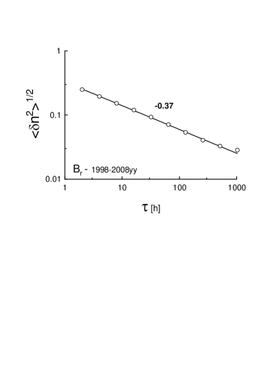
Figure 5: The standard deviation for $\delta n_{\tau}$ vs. $\tau$ for radial component $B_{r}$ of the interplanetary magnetic field, as measured by the ACE magnetometers for the last solar cycle (hourly average [17]).

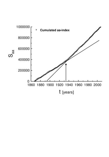
Figure 6: Cumulative aa-index vs. time. Daily aa-index was taken from [19]. The arrow indicates beginning of the transitional solar cycle.

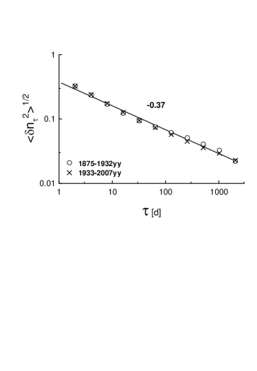
Figure 7: The standard deviation for $\delta n_{\tau}$ vs. $\tau$ (in log-log scales) for the daily aa-index [19]: circles correspond to the historic period and crosses correspond to the modern period.

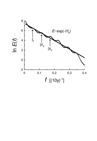
Figure 8: Spectrum of the sunspots number fluctuations in the ln-linear scales (the reconstructed data for the last 11,000 years have been taken from [20]). The straight line is drawn to indicate the exponential law Eq. (3).

Since the Rayleigh number $Ra$ of the photospheric convection preserves its order $Ra\sim 10^{11}$ with transition from the historic period to the modern one (see next Section), we can assume that just significant changes of the dynamics of the inner layers of the convection zone (most probably - of the bottom layer) were the main reasons for the transition from the historic to the modern period.

3 Magnetic fields in the solar wind and on the Earth

Although in the modern period the turbulent convection in the photosphere have no decisive impact on the sunspots emergence, the large-scale properties of the magnetic field coming through the sunspots into the photosphere and then to the interplanetary space (so-called solar wind) can be strongly affected by the photospheric motion. In order to be detected the characteristic scaling scales of this impact should be larger than the scaling scales of the interplanetary turbulence (cf. [15],[16]). In particular, one can expect that the cluster-exponent of the large-scale interplanetary magnetic field (if exists) should be close to $\alpha\simeq 0.37$. In Fig. 5 we show cluster-exponent of the large-scale fluctuations of the radial component $B_{r}$ of the interplanetary magnetic field. For computing this exponent, we have used the hourly averaged data obtained from Advanced Composition Explorer (ACE) satellite magnetometers for the last solar cycle [17]. As it was expected the cluster-exponent $\alpha\simeq 0.37\pm 0.02$. Analogous result was obtained for other components of the interplanetary magnetic field as well.

At the Earth itself the solar wind induced activity is measured by geomagnetic indexes such as aa-index (in units of 1 nT). This, the most widely used long-term geomagnetic index [18], presents long-term geomagnetic activity and it is produced using two observatories at nearly antipodal positions on the Earth’s surface. The index is computed from the weighted average of the amplitude of the field variations at the two sites. We are interested in the clustering properties of the aa-index and their relation to the modulation produced by the photospheric convective motion. The point is that the data for the aa-index are available for both the modern and the historic periods. This allows us to check the suggestion that the Rayleigh number of the photospheric convection has the same order for the both mentioned periods. The transition between the two periods is clear seen in Figure 6, where we show the cumulated aa-index $a(t)$

$$S_{aa}(t)=\int_{0}^{t}a(t^{\prime})dt^{\prime}$$

The arrow in this figure indicates beginning of the transitional solar cycle.

Figure 7 shows cluster-exponents for both the modern and the historic periods calculated for the low intensity levels of the aa-index (for the historic period the level used in the calculations is aa-index=10nT, whereas for the modern period the level is aa-index=25nT, the aa-index was taken from [19]). The low levels of intensity were chosen in order to avoid effect of the extreme phenomena (magnetic storms and etc.). The straight line in Fig. 7 is drawn to show the expected value of the cluster-exponent $\alpha\simeq 0.37$ for the both periods. It means that indeed for both the historic and the modern periods the Rayleigh number $Ra\sim 10^{11}$ (cf. Fig. 4) in the solar photosphere.

4 Chaotic sun

The long-range reconstructions of the sunspot number fluctuations (see, for instance, Refs. [1],[2]) allow us to look on the solar transitional dynamics from a more general point of view. In figure 8 we show a spectrum of such reconstruction for the last 11,000 years (the data, used for computation of the spectrum, is available at [20]). The spectrum was computed using the maximum entropy method as in Ref. [21] (see below). A semi-logarithmical representation was used in the figure to show an exponential law

$$E(f)\sim e^{-f/f_{0}}$$

The straight line is drawn in Fig. 8 to indicate the exponential law Eq. (3). Slope of the straight line provides us with the characteristic time scale $\tau=1/f_{0}\simeq 176y(\pm 7y)$. The exponential decay of the spectrum excludes the possibility of random behavior and indicates the chaotic behavior of the time series. It is well known that low-order dynamic (deterministic) systems have as a rule exponential decay of $E(f)$ in the chaotic regimes (see, for instance, [21]). As for the delay-differential equations with chaotic attractors it is interesting to compare Fig. 8 with figure 3 of the Ref. [22]. It should be noted that the 176y period is the third doubling of the period 22y. The 22y period corresponds to the Sun’s magnetic poles polarity switching.

The exponential spectrum can be also produced by a series of Lorentzian pulses with the average width of the individual pulses equals to $\tau$ (though, the distribution of widths of the pulses should be fairly narrow to result in the exponential spectrum).

In Fig. 8 a local maximum corresponding to the frequency $f_{0}$ and its first harmonics have been indicated by arrows. It should be noted that the harmonic $2f_{0}$ corresponds to the well known period $T\simeq 88y$ [23]. Comparing this with the Fig. 1 one can conclude that the period (1933y-…) of the solar hyperactivity is close to its end.

- [1] S. K. Solanki, I. G. Usoskin, B. Kromer, M. Schüssler and J. Beer, Nature, 431, 1084 (2004).
- [2] I.G. Usoskin, S.K. Solanki, M. Schüssler, et al., Phys. Rev. Lett. 91, 211101 (2003) (see also arXiv:astro-ph/0310823).
- [3] E.A. Spiegel, and N.O. Weiss, Nature, 287, 616 (1980)
- [4] A. Brandenburg, ApJ, 625 539 (2005) (see also arXiv:astro-ph/0502275).
- [5] H.W. Babcock, ApJ. 133 572 (1961).
- [6] R.B. Leighton, ApJ, 156, 1 (1969).
- [7] M. Dikpati, G.de Toma, and P.A. Gilman, Geophys. Res. Lett., 33 5102 (2006)
- [8] A.R. Choudhuri, P. Chatterjee, and J. Jiang, Phys. Rev. Lett. 98, 131101 (2007).
- [9] K.R. Sreenivasan and A. Bershadskii, J. Stat. Phys., 125, 1145 (2006).
- [10] G. Molchan, private communication.
- [11] M.R. Leadbetter and J.D. Gryer, Bull. Amer. Math. Soc. 71, 561 (1965).
- [12] Aviable at http://sidc.oma.be/sunspot-data/
- [13] R.J. Bray, R.E. Loughead, and C.J Durrant, The solar granulation (Cambridge Univ. Press, Cambridge, 2ed, 1984).
- [14] J.J. Niemela, L. Skrbek, K.R. Sreenivasan, R. J. Donnelly, Nature, 404, 837 (2000).
- [15] A. Bershadskii, Phys. Rev. Lett., 90 041101 (2003) (see also arXiv:astro-ph/0305453).
- [16] M.L. Goldstein, Space Sci. 227, 349 (2001).
- [17] Aviable at http://www.srl.caltech.edu/ACE/ASC/
- [18] P.N. Mayaud, Derivation, Meaning, and Use of Geomagnetic Indices, AGU 1129 Geophys. Monograph 22, (Washington D.C., 1980).
- [19] Aviable at http://www.ukssdc.ac.uk/data/wdcc1/wdc menu.html (World Data Centre for Solar-Terrestrial Physics, Chilton).
- [20] Aviable at http://www1.ncdc.noaa.gov/pub/data/ paleo/climate_forcing/solar_variability/usoskin-cosmic-ray.txt (see also I.G. Usoskin, K. Mursula, S.K. Solanki, M. Schuessler, and G.A. Kovaltsov, J. Geophys. Res., J. Geophys. Res., 107(A11), 1374 (2002)).
- [21] N. Ohtomo, K. Tokiwano, Y. Tanaka, A. Sumi, S. Terachi, and H. Konno, J. Phys. Soc. Jpn. 64 1104 (1995).
- [22] J. D. Farmer, Physica D, 4, 366 (1982).
- [23] J. Feynman, and S.B. Gabriel, Solar Physics, 127, 393 (1990).