Non-parametric strong lens inversion of SDSS J1004+4112

Abstract

In this article we study the well-known strong lensing system SDSS J1004+4112. Not only does it host a large-separation lensed quasar with measured time-delay information, but several other lensed galaxies have been identified as well. A previously developed strong lens inversion procedure that is designed to handle a wide variety of constraints, is applied to this lensing system and compared to results reported in other works. Without the inclusion of a tentative central image of one of the galaxies as a constraint, we find that the model recovered by the other constraints indeed predicts an image at that location. An inversion which includes the central image provides tighter constraints on the shape of the central part of the mass map. The resulting model also predicts a central image of a second galaxy where indeed an object is visible in the available ACS images. We find masses of $2.5\times 10^{13}\;M_{\odot}$ and $6.1\times 10^{13}\;M_{\odot}$ within a radius of 60 kpc and 110 kpc respectively, confirming the results from other authors. The resulting mass map is compatible with an elliptical generalization of a projected NFW profile, with $r_{\rm s}=58_{-13}^{+21}$ arcsec and $c_{\rm vir}=3.91\pm 0.74$. The orientation of the elliptical NFW profile follows closely the orientation of the central cluster galaxy and the overall distribution of cluster members.

1 Introduction

The gravitational deflection of light depends on both the luminous and dark matter present in the deflecting object, causing it to be an independent probe of the mass and possibly even the mass distribution of the deflector, i.e. the gravitational lens. Good alignment between a source, the lens and an observer, otherwise known as strong lensing, can cause several images of the source to be formed. Less perfect alignment, or weak lensing, will not cause multiple images to appear, but will still deform the image of the source somewhat. Multiple images and deformed images provide information about the mass distribution of the deflector and one can try to use these data to invert the lens, i.e. to determine its projected mass distribution.

The lensing cluster SDSS J1004+4112 was revealed by the presence of a multiply imaged quasar as reported by Inada et al. (2003). The lensing system was first identified as a quadruply imaged quasar, but later a fifth central image of the quasar was detected by Inada et al. (2005) and spectroscopically confirmed by Inada et al. (2008). Three multiply imaged galaxies were identified in HST/ACS images by Sharon et al. (2005) and time delay information for three of the quasar images was measured by Fohlmeister et al. (2008), improving the earlier reported time delay between the two closest quasar images in Fohlmeister et al. (2007). This work did not only only invalidate earlier proposed models of the lensing system (e.g. Oguri et al. (2004), Williams & Saha (2004)), which predicted shorter time delays, it also confirmed that microlensing is the cause of the strange magnification patterns in the quasar images, present both in optical (Richards et al., 2004) and X-ray (Lamer et al., 2006) measurements. With its separation of 14 arcsec, the multiply imaged quasar in SDSS J1004+4112 has held the record for being the widest lensed quasar for a number of years. The discovery of SDSS J1029+2623, a multiply imaged quasar with a separation of over 22 arcsec (Inada et al., 2006) broke this record recently. The statistics of multiply imaged quasars by clusters are studied in Hennawi et al. (2007).

In a strong lensing scenario, various kinds of information can be available, all encoding some information about the projected mass distribution of the lens. Not only does one have positional information of images of the same source, but it is also possible that magnification information or time delay information is present. Even the absence of images in certain locations can provide constraints on the mass distribution. In previous works (Liesenborgs et al. (2006), Liesenborgs et al. (2007) and Liesenborgs et al. (2008b)) we described a flexible, non-parametric method for strong lens inversion. In this article, we shall apply this procedure to SDSS J1004+4112 and compare our results with other findings about this system.

In section 2 we will review the non-parametric inversion method described in previous works, and discuss some modifications and extensions. We shall apply this method to the gravitational lensing system SDSS J1004+4112 in section 3. Finally, the results of this inversion will be discussed in section 4. Unless noted otherwise, uncertainties mentioned in this article specify a 68% confidence level.

2 Inversion method

2.1 Lensing basics

Image formation in gravitational lensing is most often described by the lens equation, which relates points $\theta$ on the image plane, describing what can be seen because of the deflection of light, to points $\beta$ on the source plane, describing what one would see without the lens effect:

$$\mbox{\boldmath$\beta$}(\mbox{\boldmath$\theta$})=\mbox{\boldmath$\theta$}-\frac{D_{\rm ds}}{D_{\rm s}}\mbox{\boldmath$\hat{\alpha}$}(\mbox{\boldmath$\theta$})\mathrm{.}$$ (1)

The angular diameter distances $D_{\rm ds}$ and $D_{\rm s}$ measure the distance between lens and source and observer and source respectively, and depend on the redshifts of source and lens. The actual bending of light rays is stored in $\hat{\alpha}$, the deflection angle.

The light travel time from source to observer is described by the time delay function:

$$t(\mbox{\boldmath$\theta$},\mbox{\boldmath$\beta$})=\frac{1+z_{\rm d}}{c}\frac{D_{\rm d}\,D_{\rm s}}{D_{\rm ds}}\left(\frac{1}{2}(\mbox{\boldmath$\theta$}-\mbox{\boldmath$\beta$})^{2}-\psi\left(\mbox{\boldmath$\theta$}\right)\right)\mathrm{.}$$ (2)

Here, $z_{d}$ describes the redshift of the gravitational lens, with corresponding angular diameter distance $D_{d}$. The gradient of the lensing potential $\psi$ is related to the deflection angle $\hat{\alpha}$ in such a way that the stationary solution of the time-delay function, i.e. $\mbox{\boldmath$\nabla$}_{\theta}t$ = 0, again yields the lens equation.

If the gravitational lens effect causes a single source to be seen as several distinct images, different light travel times will give rise to a time delay. Denoting $\beta$ the source position and $\mbox{\boldmath$\theta$}_{1}$ and $\mbox{\boldmath$\theta$}_{2}$ two corresponding image positions, the time delay between the two images is given by

$$\Delta t_{12}=t(\mbox{\boldmath$\theta$}_{1},\mbox{\boldmath$\beta$})-t(\mbox{\boldmath$\theta$}_{2},\mbox{\boldmath$\beta$})\mathrm{.}$$ (3)

If the source brightness is time-variable, similar brightness variations will be seen in the images at different times, and this time delay may be measured.

For more detailed information about the gravitational lensing formalism, the interested reader is referred to Schneider et al. (1992).

2.2 Genetic algorithm based inversion

As described in Liesenborgs et al. (2006), the inversion method we propose requires the user to specify a square-shaped region in which the procedure should try to reconstruct the projected mass density $\Sigma$ of the lens. At first, this region is subdivided into a number of smaller squares in a uniform way, and to each square a projected Plummer sphere (Plummer, 1911) is assigned. A genetic algorithm then looks for appropriate weights of these basis functions to construct a first approximation of the mass distribution. Using this first solution, a new grid is created in which regions containing more mass are subdivided further and the genetic algorithm again tries to determine appropriate weights for the associated basis functions. This iterative scheme can be repeated until the added resolution no longer considerably improves the fit to the data.

It is clear that the genetic algorithm mentioned above is the core of the inversion procedure. A genetic algorithm is an optimization strategy inspired by the Darwinian theory of evolution. An initial population of random trial solutions is evolved into solutions which are better adapted to the problem under study. To create each new generation, trial solutions are combined, cloned and mutated, and in doing so, selection pressure must be applied: trial solutions which are considered to be more fit, should create more offspring. Not only is it possible this way to create solutions which are optimized with respect to a single criterion, but so-called multi-objective genetic algorithms allow several fitness measures to be optimized at the same time. A detailed account of genetic algorithms and multi-objective genetic algorithms in particular, can be found in Deb (2001). The different fitness criteria that we use will be discussed below.

The original procedure as described in Liesenborgs et al. (2006) and Liesenborgs et al. (2007) has a shortcoming which is illustrated in Fig. 1. The left panel of this figure shows a mass map which consists of relatively small density peaks on top of a sheet of constant density. When our procedure is used to reconstruct the projected density of this lens, it fails in a quite dramatical manner (center panel). There are two causes of this undesirable behavior. First, the algorithm will have to try to mimic the effect of a mass sheet using the Plummer basis functions which is a rather difficult task, depending on the amount of constraints available. The second problem is that the subdivision scheme will be less effective. Since the mass sheet holds most of the mass, the subdivision procedure will not be successful at refining the grid in the central region.

Figure 1: Left panel: true projected mass density of a lens used to test the inversion procedure. The mass distribution consists of a few relatively small perturbations on top of a sheet of mass. Center panel: when the original procedure is applied to the images produced by the input lens, it is not successful in creating an acceptable mass map (see text). Right panel: when a sheet of mass is added as a basis function, the algorithm again is able to create acceptable reconstructions of the projected density.

To solve these problems, we have made it possible for the user to specify that the algorithm should also search for a mass sheet. In effect, we have added a mass sheet as a basis function for which the genetic algorithm needs to determine the weight. The subdivision scheme can then inspect the mass density relative to this sheet of mass so that the regions of interest can again be reconstructed with a finer resolution. The right panel of Fig. 1 illustrates how much this can help to improve the reconstruction.

The entire inversion procedure can be repeated a number of times to create a number of solutions which are compatible with the input constraints. Using such a set of solutions one can inspect the average, which highlights the common features of the mass maps, and one can calculate the standard deviation, revealing the areas in which solutions tend to disagree about the exact shape of the projected density.

2.3 Fitness criteria

2.3.1 Positions

In strong lens inversion, an obvious set of constraints is the information about multiply imaged sources. If the true mass distribution of the gravitational lens were known, using it to project the images of a single source back onto the source plane, would result in a single consistent source shape. If an incorrect lens is used, the lens equation will project each image back onto different regions in the source plane. The first fitness measure is therefore the amount of overlap between the back-projected images of each source.

Each back-projected image of a single source is surrounded by a rectangle and the distances between corresponding corners of the rectangles are used to calculate a fitness value. If corresponding points in the images can be identified, they too can be included in the fitness measure. Note that in calculating such distances, the estimated source size is used as the length scale. This avoids over-focussing the images (see Liesenborgs et al. (2006)) which is even more important when a mass sheet is included as a basis function: solutions with a considerable mass sheet will automatically project the images onto a smaller region in the source plane.

2.3.2 Null space

Using only the first criterion, the genetic algorithm evolves towards solutions for which the back-projected images overlap. However, it is also possible that other regions of the image plane are projected onto the same region in the source plane. If this is the case, the suggested solution would predict additional images. In situations where there are clearly no other images present, one would like to use this so-called null space as an additional constraint.

To do so, the null space is subdivided into a number of triangles, and the trial solution under study is used to project these triangles onto the source plane. Then, the amount of overlap between each triangle and the current estimate of the source shape is calculated and used to construct a null space fitness measure. The envelope of the back-projected images is used to estimate the source shape. More detailed information about the use of the null-space can be found in Liesenborgs et al. (2007).

2.3.3 Critical lines

In many cases it is obvious that images are not intersected by a critical line, i.e. that all points of an image have the same parity. In Liesenborgs et al. (2008b) we described how this information was used to avoid the genetic algorithm being trapped in a sub-optimal region of the solution space, where an image does get intersected by a critical line. The solution that was used simply calculated the sign of the magnification at several points inside an image, and this was used to construct a fitness measure which penalizes images in which the sign changes. While this worked well in the case of CL 0024+1654, applying the same method to SDSS J1004+4112 was far less successful.

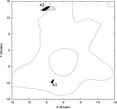
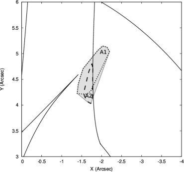
Figure 2: Illustration of the problem with the original fitness measure to penalize situations in which a critical line crosses an image. Suppose two input images (left panel, black) are known not to be intersected by a critical line. The critical lines of a certain trial solution indeed do not intersect the input images, so all the points in the input images will have the same parity. However, when the images are projected onto the source plane (right panel), the envelope of both images is in fact intersected by a caustic, causing a critical line to intersect the current prediction of the images (left panel, grey).

Fig. 2 illustrates the problem. In the left panel, the black regions mark two images of a single galaxy, and the points in each image should all have the same parity. For the constructed solution, the critical lines are shown and they clearly do not intersect the input images, meaning that no parity changes will be present in an image and that the solution will not be penalized. When the proposed mass map is used to project the images back onto the source plane, the situation in the right panel arises. Clearly, when the envelope of the back-projected images (grey area) is considered, a caustic does intersect this region and correspondingly when this shape is used to predict the images, a critical line will intersect an image as can be seen in the left panel. By not specifying precisely what type of solution one is interested in, the existing criterion can easily lead the genetic algorithm towards a sub-optimal reconstruction.

Instead of calculating the magnification information at the location of the images, the value of the magnification is now calculated on a relatively coarse grid covering the region of interest. This is used to create a rough estimate of the critical lines, which in turn are projected onto the source plane to provide an estimate of the caustics. The intersection of the caustics with the source shape is calculated and the total length is used as a fitness measure, a lower value indicating a better fitness.

2.3.4 Time delay information

When time delay information is available for a number of images of a single source, one would like to use this information to constrain the allowed region in the solution space even further. By calculating the lensing potential at the image points for which time delay information is available, in principle equation (2) can be used to compare the predicted time delays with the observed ones. However, to do so, one needs to know the position $\beta$ of the source. While the source position may be estimated once a good overlap of the images has been reached, this is in general not possible while the genetic algorithm is still evolving, and certainly not near the start, when the trial mass maps are still quite random and the images are projected onto very different regions.

Having tested a number of possible fitness measures, we found that the following one works very well. Suppose that there are $N$ images $\mbox{\boldmath$\theta$}_{i}$ with corresponding points in the source plane $\mbox{\boldmath$\beta$}_{i}$. It is possible that time delay information is not available for all images, so let us call $T$ the set of image indices for which time delay information is at hand. The measured time delay between image $i$ and $j$ will be called $\Delta t_{{\rm obs},ij}$. The fitness measure is then given by:

$$\sum_{i\in T}\sum_{\begin{subarray}{c}j\in T\\ j\neq i\end{subarray}}\sum_{k=1}^{N}\sum_{l=1}^{N}\left(\frac{\left[t(\mbox{\boldmath$\theta$}_{i},\mbox{\boldmath$\beta$}_{k})-t(\mbox{\boldmath$\theta$}_{j},\mbox{\boldmath$\beta$}_{l})\right]-\Delta t_{{\rm obs},ij}}{\Delta t_{{\rm obs},ij}}\right)^{2}\mathrm{.}$$ (4)

Again, a lower value implies a better fitness of the trial solution.

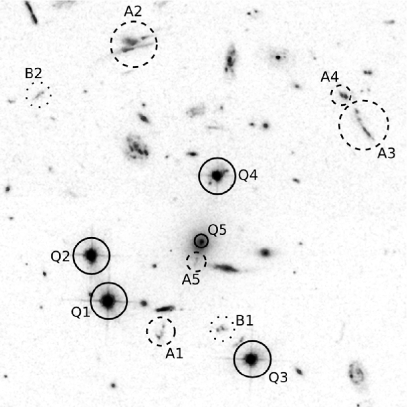
Figure 3: The multiple image systems which are used in the inversion of SDSS J1004+4112, using the same labeling as Sharon et al. (2005) (north is up, east is left). Five images of a quasar (Q1-Q5) are available, as well as four, possibly five images of a galaxy marked A1-A5, and two images of a second galaxy marked B1-B2. Between B1 and Q3 and to the left of B2 are two images of a third galaxy marked C1-C2 in Sharon et al. (2005), but this system was not used as no redshift is currently available.

Figure 4: Left panel: when the input images are projected back on to the source plane using the average of 28 individual solutions, these source positions are obtained. Galaxy A is surrounded by a dashed rectangle, galaxy B by a dotted one. The caustics correspond to the redshift of the quasar. Right panel: when the sources and caustics of the left panel are used to predict the images and critical lines using the average solution, this configuration is obtained.

Figure 5: Left panel: average mass map of 28 individual solutions when image A5 is not taken into account. Most of the mass is found to coincide with the region of the BCG. The critical density was calculated at the redshift of the quasar. Right panel: standard deviation of the individual solutions, showing that the precise distribution near the center of the cluster is somewhat uncertain.

3 Application to SDSS J1004+4112

3.1 Multiple image systems

Fig. 3 shows the image systems that were used in the inversion of SDSS J1004+4112, using the same labeling as Sharon et al. (2005). There are five spectroscopically confirmed images of a quasar at redshift $1.734$, labeled Q1-Q5. Corresponding to the time delay measurements of Fohlmeister et al. (2008), we used a time delay of 40.6 days between Q2 and Q1, and a time delay of 821.6 days between Q3 and Q1. No magnification information was used, as the quasar image magnifications are influenced by microlensing, introducing a large uncertainty. The positions of the quasar images were set to those reported in Inada et al. (2005). Four, possibly five images are present of a galaxy at redshift $3.332$, labeled A1-A5, with image A5 being marked as uncertain by Sharon et al. (2005). The third system used consists of two images of a galaxy at redshift $2.74$, marked B1-B2. Note that another galaxy with two images was identified in the aforementioned work, but because of its unknown redshift, it was not used in the inversion. Angular diameter distances were calculated in a flat cosmological model with $H_{0}=71$ km s^-1 Mpc^-1, $\Omega_{\rm m}=0.27$ and $\Omega_{\Lambda}=0.73$. Using the redshift information described above, this fixes the $D_{ds}/D_{s}$ ratios for the lensing systems, which is required input information in our method.

Figure 6: The circularly averaged profile of the inversions when image A5 is disregarded, together with the standard deviation.

Figure 7: The central part of the cluster after removing the contribution of the central cluster members using GALFIT. The central quasar image can clearly be seen in each filter, in the upper left part of the image. Below and to the left of it, image A5 can be seen in the F555W and F814W images. More to the right, an extra object can be seen, where the inversion predicts the central images of galaxies B and C.

3.2 First inversion

Since image A5 was marked as uncertain, the first inversion does not include it. The algorithm was instructed to look for mass in a square region, 35 arcsec wide, roughly centered on image Q4. The null space fitness measure was based on a square region, 60 arcsec wide, subdivided into a 64 by 64 grid. For each source, the image regions were excluded from the null space, and for systems A and B, the central cluster region was excluded as well, allowing the algorithm to predict the locations of the central images of these systems. The null space is a relatively large region, but this avoids the introduction of unnecessary substructure at the edge of the mass reconstruction region, that would cause images to appear at larger distances. The critical line fitness was based on a square shaped region, 40 arcsec wide, subdivided into a 64 by 64 grid. After each inversion, a finalizing step was performed, as described in Liesenborgs et al. (2008b). This causes some minor modifications to be made to the mass map, to improve the positional and time delay fitness measures. In the same work we described how mass could be redistributed without affecting any of the observable properties and demonstrated this on the obtained mass map for Cl 0024+1654. In this work however, no explicit mass redistribution step is performed.

The average solution of 28 individual inversions predicts the source positions and caustics shown in the left panel of Fig. 4. The source position of galaxy A is marked by a dashed rectangle, the position of galaxy B is marked by a dotted one. When these sources and the reconstructed lens are used to predict the image configurations, the result in the right panel of the same figure is obtained. The critical lines and caustics in these figures are calculated for the redshift of the quasar. The mass map itself is shown in the left panel of Fig. 5, with most of the mass in the same region as the brightest cluster galaxy (BCG). The standard deviation of the individual reconstruction can be seen in the right panel of the same figure, showing that the precise distribution of mass in the central region differs between the individual reconstructions. Fig. 6 shows the average profile and its standard deviation. The large core clearly differs from the NFW-like behavior that one might expect.

When inspecting the right panel of Fig. 4, one sees that the average solution predicts central images of galaxies A and B. The predicted position of the central image of galaxy A coincides with the location of image A5, although the predicted shape is far less extended. Fig. 7 shows the central region of the cluster, after subtracting the central cluster members using the GALFIT software (Peng et al., 2002). In each of the filters, one can clearly see the central image of the quasar in the upper-left region. Image A5 can clearly be seen in the F555W and F814W images. Since the other constraints predict a central image of galaxy A at this location and since it indeed resembles a mirror image of A1, we feel confident that this is in fact the central image of galaxy A.

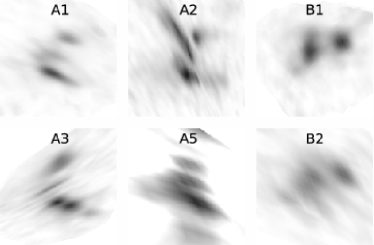
Figure 8: When using the model resulting from the second inversion to project the galaxy images back onto their source planes, these images are obtained. Note that image A4 is not shown here, as it is occluded by a cluster galaxy. The size of galaxy A is approximately 4 kpc, the size of galaxy B is approximately 2.5 kpc.

Figure 9: Left panel: when the average of 28 individual solutions is used to reconstruct the source plane when image A5 is included as a constraint, this result is obtained. The dashed box again indicates galaxy A, the dotted one galaxy B. Right panel: the sources and caustics in the left panel correspond to these images and critical lines. In this case, the central image of galaxy A is indeed more elongated. The critical lines and caustics again correspond to the redshift of the quasar.

Figure 10: Left panel: average mass density of the 28 individual solutions. When image A5 is included, the central region clearly needs to be much steeper. Right panel: standard deviation of the individual solutions. The precise mass distribution in the central region differs somewhat among the reconstructions. The critical density again corresponds to the critical density at the redshift of the quasar.

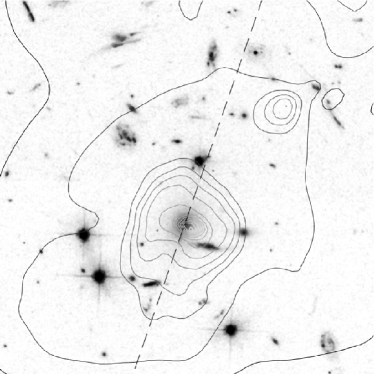
Figure 11: The average solution resulting from the second inversion is shown as a contour map on top of the ACS image. Most of the mass clearly lies in the same area as the central cluster members. The mass peak in the north-west part of the figure is not significant, as it can easily be redistributed. The dashed line indicates the orientation of the BCG.

Figure 12: Left panel: average profile and standard deviation of the resulting mass distributions. The dashed line shows the best fit NFW profile. Right panel: when only the mass density at the location of the images is taken into account, this is the resulting best fit NFW. The center of the profile lies very close to Q5, as does the center of the BCG. The orientation is very similar to that of the BCG (dashed line), and corresponds to the general alignment of the cluster members (Oguri et al., 2004).

3.3 Second inversion

Including the central image of galaxy A will provide additional information that will lead to a different inversion since its true shape is different from the one predicted by the first inversion. For this reason, a second inversion was performed in which image A5 was added as an observational constraint. The rest of the constraints are the same as in the first inversion. Fig. 9 shows the source and image configurations obtained in this case, using the average solution of 28 individual reconstructions. The central image of galaxy A is now clearly more extended than in the first inversion. When the images of galaxies A and B are projected back onto their source planes, the source shapes in Fig. 8 are reconstructed. The back-projected images of each source clearly resemble each other, illustrating that a good positional fitness has been achieved. The estimated size of galaxy A is approximately 4 kpc, the size of galaxy B approximately 2.5 kpc.

The effect of the inclusion of image A5 can best be seen in the average mass map, as shown in the left panel of Fig. 10. Now, the mass distribution has clearly become much steeper in the central region, although some disagreement still remains between the individual solutions (right panel). A comparison with the visible matter can be seen in Fig. 11. The effect on the mass density can also be clearly seen in the circularly averaged profile, shown in the left panel of Fig. 12. It would definitely be interesting to see how much the resulting mass map resembles a NFW distribution.

The NFW density profile (Navarro et al., 1996) is described by:

$$\rho_{\rm NFW}(r)=\frac{\rho_{\rm s}}{(r/r_{\rm s})(1+r/r_{\rm s})^{2}}\mathrm{,}$$ (5)

in which $\rho_{\rm s}$ is a density scale factor and $r_{\rm s}$ is a characteristic radius. The density scale can be expressed in terms of $c_{\rm vir}$, which relates $r_{\rm s}$ to the virial radius $r_{\rm vir}$ through $r_{\rm vir}=c_{\rm vir}r_{\rm s}$. The virial radius itself is defined as the radius within which the mean density equals $\Delta_{\rm vir}$ times the mean matter density at the redshift of the halo. This virial overdensity $\Delta_{\rm vir}$ stems from the spherical collapse model, and for a flat cosmological model it can be approximated by (e.g. Bryan & Norman (1998), Bullock et al. (2001))

$$\Delta_{\rm vir}\approx\frac{18\pi^{2}+82x-39x^{2}}{\Omega(z)}\mathrm{,}$$ (6)

in which $x=\Omega(z)-1$ and $\Omega(z)$ is defined as the ratio of the mean matter density to the critical density. Through lens inversion one recovers the projected density:

$$\Sigma_{\rm NFW}(R)=\int_{-\infty}^{\infty}\rho_{\rm NFW}(R,z)dz\mathrm{,}$$ (7)

for which an analytical expression can be calculated (e.g. Wright & Brainerd (2000)).

	Prediction	CASTLES			I2005	F2008
Image		F160W	F555W	F814W
Q1	1	1	1	1	1	1
Q2	$1.03\pm 0.38$	0.6486	1.0864	1.3428	0.732	0.724
Q3	$0.54\pm 0.19$	0.4487	0.4529	0.4656	0.346	0.592
Q4	$0.29\pm 0.11$	0.3191	0.6138	0.2489	0.207
Q5	$0.032\pm 0.029$	0.0114	0.00024	0.0047	0.003

Table 1: The predicted flux ratios of the quasar images, compared to data from the CASTLES project, Inada et al. (2005) and Fohlmeister et al. (2008) respectively. Note that only in this last work, the combined effect of the intrinsic variability of the source and the time delay has been taken into account. The general trend of the predicted values matches the observations, even though no magnification information was used in the inversion. The uncertainties show that this non-parametric inversion method can create a wide variety of flux ratios, even without having to consider microlensing.

Naively performing a fit of the profile in the left panel of Fig. 12 to a projected NFW profile, yields the best fit profile described by the dashed line in the same figure. One then finds $r_{\rm s}=41.2_{-1.3}^{+1.5}$ arcsec, and $c_{\rm vir}=5.37_{-0.12}^{+0.14}$. Although this seems to correspond well to the values found by Ota et al. (2006), who reported $r_{\rm s}=39_{-9}^{+12}$ arcsec and $c_{\rm vir}=6.1_{-1.2}^{+1.5}$ (90% confidence) based on Chandra X-ray observations, the uncertainties found in this way are far too low. As explained in Liesenborgs et al. (2008b), using the monopole degeneracy it is possible to redistribute the mass in between the images, without affecting any of the observable properties of the lensing system. This means that the uncertainty of the circularly averaged profile is actually much larger than obtained by simply calculating the standard deviation of the individual profiles. In turn, this translates to larger uncertainties on the parameters of the fit.

Since the mass distribution in between the images is not well constrained, it is interesting to see how much the density at the location of the images themselves constrains the NFW parameters. First, we calculated the average density and its standard deviation at the location of each image. Then, an elliptical generalization of $\Sigma_{\rm NFW}$ was fitted to these data points. An axis ratio $f$ was introduced in the projected NFW profile by setting $R=(fx^{2}+y^{2}/f)^{1/2}$ in equation (7). We prefer this substitution over $R=(x^{2}+(y/q)^{2})^{1/2}$ that would correspond to an axisymmetric NFW instead of a triaxial one, because the circularly averaged profile in the first case corresponds closely to the profile of a symmetric NFW with the same $r_{\rm s}$ and $c_{\rm vir}$ parameters. This allows the obtained values to be compared directly to fits to the circularly averaged profile. After fitting the elliptical generalization of $\Sigma_{\rm NFW}$, the values $r_{\rm s}=58_{-13}^{+21}$ arcsec and $c_{\rm vir}=3.91\pm 0.74$ are obtained. The best fit NFW is shown in the right panel of Fig. 12. Its orientation corresponds to that of the BCG and to the general configuration of the cluster members as reported in Oguri et al. (2004).

When calculating the total mass within 60 kpc, corresponding to the region of the quasar images, and 110 kpc, the region bounded by the images of galaxy A, we find results of $2.5\times 10^{13}\;M_{\odot}$ and $6.1\times 10^{13}\;M_{\odot}$ respectively. These values can be compared to the findings of Williams & Saha (2004), who also find $2.5\times 10^{13}\;M_{\odot}$, and of Sharon et al. (2005), who find $6\times 10^{13}\;M_{\odot}$. This illustrates once more that the mass within the images is well constrained.

In Sharon et al. (2005) a lens model was used to predict the redshift of galaxy C, of which the two images lie between B1 and Q3, and to the left of B2 respectively (see Fig. 3). Doing the same using the average model discussed above, we find that the back-projected images nearly overlap for a $D_{\rm ds}/D_{\rm s}$ ratio of 0.64, corresponding to a redshift of 3.35, slightly higher than the reported redshift of 2.94. After the inversions were completed, we have learned that the authors of the aforementioned work have now spectroscopically confirmed the redshift of galaxy C to be 3.288 (private communication).

The right panel of Fig. 9 contains a prediction for the central image of galaxy B, lying to the right of image A5. Inspecting Fig. 7 again, there indeed seems to be an object at that location, which is especially clear in the F435W and F555W filters. It is important to note however that the model also predicts that the central image of galaxy C mentioned above, is located at almost the same location as the central image of galaxy B. For this reason, the object that can be seen in Fig. 7, is possibly a superposition of the central images of these two galaxies.

The predicted flux ratios for the quasar system – relative to the flux of Q1 – are shown in table 1 and are compared to the flux ratios from other works. Although no magnification information was used in the inversion, the general trend of the predictions matches the observations. Also note that the relatively large uncertainties show that the non-parametric technique can accomodate a wide number of flux ratios, without taking microlensing into account. Finally, the model presented here predicts a time delay of slightly over 1300 days between images Q1 and Q4 of the quasar. This is still consistent with the constraint presented in Fohlmeister et al. (2008) which specifies that this delay should be over 1250 days. The Q1-Q5 time delay is predicted to be of the order of 1900 days.

4 Discussion and conclusions

In this article we have applied a previously developed strong lens inversion method to the case of SDSS J1004+4112. The constraints used include time delay information, positional information and null-space information, all handled well using a multi-objective genetic algorithm.

The system under study only provides a few sources at different redshifts, which, in principle, still allows a generalized version of the mass sheet or steepness degeneracy (Liesenborgs et al., 2008a). It is for this reason that the available time delay information is of particular importance here, as it directly breaks the degeneracy. The fact that the degeneracy is broken well can be seen in the low dispersion in the outer regions of the surface density (right panels of Figs. 5 and 10) which is of the order of $\Sigma/\Sigma_{cr}\approx 0.05$, indicating that in our extended version of the genetic algorithm a similar mass sheet basis function is found in each individual reconstruction. It is interesting to compare the mass map of the second inversion to the mass map obtained by Saha et al. (2007). The outer contours of their reconstruction show a remarkably circular structure, causing a similar effect as the mass sheet basis function used in our work. The contour steps in that figure would correspond to $\Sigma/\Sigma_{\rm cr}=0.22$, indicating that a similar mass density will be found near the edges of image system A as in our work.

Note that in the reconstruction of the projected mass density, relatively large structures seem to exist to the north and south of images A3 and A4. As already suggested by the large associated standard deviations, one should not place much confidence in the displayed shape of these features, as the mass in those regions can easily be redistributed without affecting any of the observable properties of the lensing system using the monopole degeneracy (Liesenborgs et al., 2008b). For the same reason it is extremely difficult to make reliable statements about the nature of substructure that may be present near the cluster center. One can only hope to make reliable predictions about the projected density at the location of the images themselves, illustrating the need for lenses with many multiply-imaged systems. Furthermore, to probe the core regions of clusters, central images are of particular importance as is nicely illustrated by the difference in profiles between the two inversions shown in this article.

When studying the constraints provided by the density at the image locations, we find that the resulting best fit NFW bears great resemblence to the general cluster configuration. As is often the case (e.g. Keeton et al. (1998)) the fit has a very similar orientation as that of the central galaxy, which in this case also follows the general distribution of the cluster galaxies. In a recent study, Oguri et al. (2009) discussed the fact that lensing clusters are often over-concentrated. Although the circularly averaged profile indeed suggests that this may be the case in this cluster as well, the more reliable two-dimensional fit yields an estimate of the concentration which is compatible with the expected value $c_{\rm vir}\sim 4$.

The method described and applied in this article is a non-parametric one, in the sense that no predefined shape for the matter distribution is used to fit the data. This is done by arranging a large number of Plummer basis functions on a grid. In a recent article, Jullo & Kneib (2009) made the interesting point that when basis functions overlap, the introduced correlation reduces the effective number of degrees of freedom, making such a non-parametric inversion less underconstrained than it appears at a first glance. In any case, non-parametric methods can certainly help to explore a larger portion of the solution space, helping one to obtain a less biased look at the possible mass distributions. As with any method, one must be cautious about interpreting the results, since degeneracies can greatly enhance the uncertainties involved.

References

- Bryan & Norman (1998) Bryan G. L., Norman M. L., 1998, ApJ, 495, 80
- Bullock et al. (2001) Bullock J. S., Kolatt T. S., Sigad Y., Somerville R. S., Kravtsov A. V., Klypin A. A., Primack J. R., Dekel A., 2001, MNRAS, 321, 559
- Deb (2001) Deb K., 2001, Multi-Objective Optimization Using Evolutionary Algorithms. John Wiley & Sons, Inc., New York, NY, USA
- Fohlmeister et al. (2008) Fohlmeister J., Kochanek C. S., Falco E. E., Morgan C. W., Wambsganss J., 2008, ApJ, 676, 761
- Fohlmeister et al. (2007) Fohlmeister J., Kochanek C. S., Falco E. E., Wambsganss J., Morgan N., Morgan C. W., Ofek E. O., Maoz D., Keeton C. R., Barentine J. C., Dalton G., Dembicky J., Ketzeback W., McMillan R., Peters C. S., 2007, ApJ, 662, 62
- Hennawi et al. (2007) Hennawi J. F., Dalal N., Bode P., 2007, ApJ, 654, 93
- Inada et al. (2008) Inada N., Oguri M., Falco E. E., Broadhurst T. J., Ofek E. O., Kochanek C. S., Sharon K., Smith G. P., 2008, PASJ, 60, L27+
- Inada et al. (2005) Inada N., Oguri M., Keeton C. R., Eisenstein D. J., Castander F. J., Chiu K., Hall P. B., Hennawi J. F., Johnston D. E., Pindor B., Richards G. T., Rix H.-W. R., Schneider D. P., Zheng W., 2005, PASJ, 57, L7
- Inada et al. (2006) Inada N., Oguri M., Morokuma T., Doi M., Yasuda N., Becker R. H., Richards G. T., Kochanek C. S., Kayo I., Konishi K., Utsunomiya H., Shin M.-S., Strauss M. A., Sheldon E. S., York D. G., Hennawi J. F., Schneider D. P., Dai X., Fukugita M., 2006, ApJ, 653, L97
- Inada et al. (2003) Inada N., Oguri M., Pindor B., Hennawi J. F., Chiu K., Zheng W., Ichikawa S.-I., Gregg M. D., Becker R. H., Suto Y., Strauss M. A., Turner E. L., Keeton C. R., Annis J., Castander F. J., Eisenstein D. J., Frieman J. A., Fukugita M., Gunn J. E., Johnston D. E., Kent S. M., Nichol R. C., Richards G. T., Rix H.-W., Sheldon E. S., Bahcall N. A., Brinkmann J., Ivezić Ž., Lamb D. Q., McKay T. A., Schneider D. P., York D. G., 2003, Nat, 426, 810
- Jullo & Kneib (2009) Jullo E., Kneib J.-P., 2009, ArXiv e-prints
- Keeton et al. (1998) Keeton C. R., Kochanek C. S., Falco E. E., 1998, ApJ, 509, 561
- Lamer et al. (2006) Lamer G., Schwope A., Wisotzki L., Christensen L., 2006, in ESA Special Publication, Vol. 604, The X-ray Universe 2005, Wilson A., ed., pp. 641–+
- Liesenborgs et al. (2006) Liesenborgs J., De Rijcke S., Dejonghe H., 2006, MNRAS, 367, 1209
- Liesenborgs et al. (2007) Liesenborgs J., De Rijcke S., Dejonghe H., Bekaert P., 2007, MNRAS, 380, 1729
- Liesenborgs et al. (2008a) Liesenborgs J., De Rijcke S., Dejonghe H., Bekaert P., 2008a, MNRAS, 386, 307
- Liesenborgs et al. (2008b) Liesenborgs J., De Rijcke S., Dejonghe H., Bekaert P., 2008b, MNRAS, 389, 415
- Navarro et al. (1996) Navarro J. F., Frenk C. S., White S. D. M., 1996, ApJ, 462, 563
- Oguri et al. (2009) Oguri M., Hennawi J. F., Gladders M. D., Dahle H., Natarajan P., Dalal N., Koester B. P., Sharon K., Bayliss M., 2009, ArXiv e-prints
- Oguri et al. (2004) Oguri M., Inada N., Keeton C. R., Pindor B., Hennawi J. F., Gregg M. D., Becker R. H., Chiu K., Zheng W., Ichikawa S.-I., Suto Y., Turner E. L., Annis J., Bahcall N. A., Brinkmann J., Castander F. J., Eisenstein D. J., Frieman J. A., Goto T., Gunn J. E., Johnston D. E., Kent S. M., Nichol R. C., Richards G. T., Rix H.-W., Schneider D. P., Sheldon E. S., Szalay A. S., 2004, ApJ, 605, 78
- Ota et al. (2006) Ota N., Inada N., Oguri M., Mitsuda K., Richards G. T., Suto Y., Brandt W. N., Castander F. J., Fujimoto R., Hall P. B., Keeton C. R., Nichol R. C., Schneider D. P., Eisenstein D. E., Frieman J. A., Turner E. L., Minezaki T., Yoshii Y., 2006, ApJ, 647, 215
- Peng et al. (2002) Peng C. Y., Ho L. C., Impey C. D., Rix H.-W., 2002, AJ, 124, 266
- Plummer (1911) Plummer H. C., 1911, MNRAS, 71, 460
- Richards et al. (2004) Richards G. T., Keeton C. R., Pindor B., Hennawi J. F., Hall P. B., Turner E. L., Inada N., Oguri M., Ichikawa S.-I., Becker R. H., Gregg M. D., White R. L., Wyithe J. S. B., Schneider D. P., Johnston D. E., Frieman J. A., Brinkmann J., 2004, ApJ, 610, 679
- Saha et al. (2007) Saha P., Williams L. L. R., Ferreras I., 2007, ApJ, 663, 29
- Schneider et al. (1992) Schneider P., Ehlers J., Falco E. E., 1992, Gravitational Lenses. Springer-Verlag
- Sharon et al. (2005) Sharon K., Ofek E. O., Smith G. P., Broadhurst T., Maoz D., Kochanek C. S., Oguri M., Suto Y., Inada N., Falco E. E., 2005, ApJ, 629, L73
- Williams & Saha (2004) Williams L. L. R., Saha P., 2004, AJ, 128, 2631
- Wright & Brainerd (2000) Wright C. O., Brainerd T. G., 2000, ApJ, 534, 34