CRETE-09-11

UFIFT-QG-09-02

A Phenomenological Model for the Early Universe

N. C. Tsamis^†

Department of Physics, University of Crete
GR-710 03 Heraklion, HELLAS.

R. P. Woodard^∗

Department of Physics, University of Florida
Gainesville, FL 32611, UNITED STATES.

ABSTRACT

We consider the description of cosmological dynamics from the onset of inflation by a perfect fluid whose parameters must be consistent with the strength of the enhanced quantum loop effects that can arise during inflation. The source of these effects must be non-local and a simple incarnation of it is studied both analytically and numerically. The resulting evolution stops inflation in a calculable amount of time and leads to an oscillatory universe with a vanishing mean value for the curvature scalar and an oscillation frequency which we compute.

PACS numbers: 04.60.-m, 04.62.+v, 98.80.Cq

^† e-mail: tsamis@physics.uoc.gr

^∗ e-mail: woodard@phys.ufl.edu

1 Introduction

Although it is not yet known how to account for the late time acceleration of the universe [1, 2], it is by now quite clear that an adequate period of approximately exponential expansion – inflation [3] – provides a simple and natural explanation for the homogeneity and isotropy of the large-scale observable universe [4], and also is in satisfactory agreement with the primordial density perturbations spectrum [5]. This inflationary phase is usually realized by a scalar field but this is not a necessity.

Consider the pure gravitational equations of motion:

$$G_{\mu\nu}\;\equiv\;R_{\mu\nu}\,-\,\frac{1}{2}g_{\mu\nu}\,R\;=\;-\Lambda\,g_{\mu\nu}\;\;.$$ (1)

If $\Lambda$ is assumed to be positive, the “no-hair” theorems imply that classically the local geometry approaches the maximally symmetric solution at late times [6]; this solution is de Sitter spacetime and, thus, $\Lambda$-driven inflation is intrinsic to (1).

As (1) shows, classical gravitation without matter is a theory which only “knows” about the cosmological constant $\Lambda\,$; Newton’s constant $G$ sets the strength of quantum effects. The corresponding mass scales are the Planck mass $M_{\rm Pl}$ – associated with $G$ – and the mass $M$ – associated with $\Lambda$:

$$M^{2}_{\rm Pl}\;\equiv\;\frac{1}{G}\qquad,\qquad M\;\equiv\;\Big{(}\frac{\Lambda}{8\pi G}\Big{)}^{\frac{1}{4}}\;\;.$$ (2)

We restrict ourselves to scales below the Planck mass so that the dimensionless coupling constant $\epsilon\equiv G\Lambda$ of the theory is small:

$$M\;<\;M_{\rm Pl}\qquad\Longleftrightarrow\qquad\epsilon\,\equiv\,G\Lambda\;<\;1\;\;.$$ (3)

The quantum behaviour of gravity in de Sitter ($dS$) spacetime has been studied in perturbation theory and in the infrared [7, 8]. In particular, the expansion rate $H(t)$ decreases by an amount which becomes non-perturbatively large at late times:

$$de\;Sitter\quad\Longrightarrow\quad H(t)\;\simeq\;H_{0}\left\{1\,-\,\epsilon^{2}\Big{[}\,\#(H_{0}\,t)+O(1)\,\Big{]}\,+\,O(\epsilon^{3})\right\}\;\;,$$ (4)

where $\#$ is a positive pure number of $O(1)$. The underlying physical mechanism is the production of infrared quanta out of the vacuum due to the accelerated expansion of spacetime. Such a production can only occur for particles that are light compared to the Hubble scale without classical conformal invariance; gravitons and massless minimally coupled scalars are unique in that respect.

The factor of $H_{0}\,t$ which appears in expression (4) is known as an infrared logarithm because it derives from infrared virtual particles and because $H_{0}\,t$ is the logarithm of the de Sitter scale factor. Any quantum field theory which involves undifferentiated gravitons or massless minimally coupled scalars will show infrared logarithms in some correlators at some order in the loop expansion. If the interaction contains $N$ undifferentiated gravitons or massless minimally coupled scalars, along with any number of other fields, then each new factor of the coupling constant squared can produce at most $N$ additional infrared logarithms. For example, the fundamental interaction of quantum gravity in de Sitter background takes the generic form [9]:

$$\sqrt{G}\;h\,\partial h\,\partial h\;\;,$$ (5)

where $h_{\mu\nu}$ is the fluctuating graviton field. Thus, one can get at most one extra infrared logarithm for each additional power of $G$ [8].

The operator under study also has an effect. For example, because there are two derivatives in the invariant measure of acceleration [10] whose expectation value gave expression (4), the general form of such corrections is:

$$H(t)\;=\;H_{0}\,\Biggl{\{}1\,-\,\sum_{\ell=2}^{\infty}\epsilon^{\ell}\,\sum_{k=0}^{\ell-1}c_{\ell k}\,(H_{0}\,t)^{k}\Biggr{\}}\;\;,$$ (6)

where $\ell$ stands for the loop order and where the constants $c_{\ell k}$ are pure numbers of $O(1)$.

Because $\epsilon$ is constant, whereas $H_{0}\,t$ grows without bound, infrared logarithms eventually lead to a breakdown of perturbation theory. In quantum gravity on de Sitter background this occurs after about $\epsilon^{-1}$ e-foldings. To evolve further requires a non-perturbative technique such as summing the series of leading infrared logarithms:

$$H(t)\Big{|}_{\rm leading\;log}\;=\;H_{0}\,\Biggl{\{}1\,-\,\epsilon\sum_{\ell=2}^{\infty}c_{\ell,\,\ell-1}\;(\epsilon H_{0}\,t)^{\ell-1}\Biggr{\}}\;\;.$$ (7)

Starobinskiĭ [11] has developed a stochastic technique which exactly reproduces the leading infrared logarithms of scalar potential models [8], and which can be used to sum them whenever the scalar potential is bounded below [12]. Starobinskiĭ’s technique has recently been extended to include models in which the scalar interacts with other fields such as a Yukawa fermion [13] or electromagentism [14]. The late time limits of the vacuum energies of these scalar models exhibit a broad range of possibilities for what the quantum gravitational sum might give:

• Scalar potential models which are bounded below show a small, constant increase of the vacuum energy [12, 15];

• Scalar quantum electrodynamics experiences a small, constant decrease of the vacuum energy [14]; and

• Yukawa theory engenders a decrease of the vacuum energy which grows without bound [13].

We would ultimately like to compute how quantum gravity affects late time cosmology by employing Starobinskiĭ’s technique to sum the series of leading infrared logarithms. There has been some progress in this area [16] but the full solution is not yet in sight. A more modest approach is to anticipate the solution by attempting to guess the most cosmologically significant part of the effective field equations guided by our understanding of the perturbative regime at leading logarithm order. The resulting model could be regarded as a worthy object of study in its own right, just as one views the many classes of scalar-driven inflation models, without feeling any need to derive them from fundamental theory. It may even be that our study will uncover some general feature of any successful model which can, it turn, guide the fundamental derivation.

It should be noted that doubts have been raised about the possibility of any infrared contribution to the quantum gravitational vacuum energy [17, 18]. However, these doublts are difficult to reconcile with the fact that scalar models certainly show infrared corrections to the vacuum energy [12, 15, 14, 13], and with Weinberg’s observation that infrared logarithms contaminate the power spectrum of scalar-driven inflation [19]. General theoretical arguments have also been advanced to show that de Sitter must be unstable in quantum gravity [20].

One feature which complicates evaluation of these arguments is the intractibility of quantum gravity at any order, and the fact that the onset of this particular effect occurs at two loops. The latter fact must be so because screening represents the gravitational attraction between virtual infrared gravitons which have been ripped from the vacuum. The production process is a one-loop effect, so the gravitational response to it cannot occur until the next loop order. Three separate computations of the graviton 1-point function have confirmed that there is no one-loop effect [21, 22, 23], and the same conclusion can be reached from taking the de Sitter limit of scalar-driven inflation [24, 25]. This difficulty of performing explicit computations is one more reason why it might be desirable to study quantum gravitational screening from the perspective of the effective field equations.

In the present paper we shall use the physical principles responsible for the non-trivial quantum gravitational back-reaction on inflation to construct a phenomenological model which we can then directly evolve. Therefore, we wish to construct an appropriate effective conserved stress-energy tensor $T_{\mu\nu}[g]$ which will modify the gravitational equations of motion (1) in the usual way:

$$G_{\mu\nu}\;=\;-\Lambda\,g_{\mu\nu}\,+\,8\pi G\,T_{\mu\nu}[g]\;\;.$$ (8)

Our stress-energy tensor must be a non-local functional of the metric as dictated by the nature of the effect we wish to describe. It can be conveniently parametrized as a “perfect fluid”:

$$T_{\mu\nu}[g]\;=\;(\rho+p)\,u_{\mu}\,u_{\nu}\,+\,p\,g_{\mu\nu}\;\;,$$ (9)

so that to completely determine it we need the following three ingredients:
(i) the energy density $\rho$ as a functional of the metric tensor $\rho[g](x)$,
(ii) the pressure $p$ as a functional of the metric tensor $p[g](x)$,
(iii) the 4-velocity field $u_{\mu}$ as a functional of the metric tensor $u_{\mu}[g](x)$, chosen to be timelike and normalized:

$$g^{\mu\nu}\,u_{\mu}u_{\nu}=-1\qquad\Longrightarrow\qquad u^{\mu}\,u_{\mu;\nu}=0\;\;.$$ (10)

Section 2 describes a simple ansatz for the effective stress-energy tensor $T_{\mu\nu}[g]$ and the set of equations it leads to for homogeneous and isotropic spacetimes. Section 3 presents numerical results obtained by discretizing the relevant evolution equation. To the degree that is possible, the dynamics of homogeneous and isotropic evolution in the presence of $T_{\mu\nu}[g]$ is studied analytically in Section 4 and – wherever a comparison can be made – the excellent agreement with our numerical study is noticed. Section 5 discusses late time evolution and the possible modifications it implies on our ansatz. Our conclusions comprise Section 6.

2 A Physical Ansatz

It is clearly impossible to uniquely fix the functional form of the effective stress-energy tensor solely from the physical requirements and correspondence limits we have at our disposal; only quantum field theory could, in principle, provide such an answer. However, we can try to obtain a simple ansatz and then analyze its implications.

$\bullet\;\;$ Why a Perfect Fluid?
One might think that a good way of discussing quantum corrections to the field equations would be in terms of an ansatz for the effective action. However, the “in-out” effective action – being non-local – does not give causal effective field equations we can use to study cosmological evolution. The “in-in” effective action of the Schwinger-Keldysh formalism does produce causal effective field equations, but this results from subtle cancellations between different off-shell fields, making it difficult to identify promising candidates for the off-shell effective action. For a class of simple non-local effective actions, it is possible – using a partial integration “trick” – to obtain causal effective field equations [27] but it is impossible to restrict the non-local effects to the past. The chain of action and reaction that is part of any single-field variational formalism implies that screening the cosmological constant by an inverse differential operator acting on some curvature scalar will inevitably lead to a variation of that curvature scalar appearing at the current time in the effective field equations. Hence one always gets a renormalization of the effective Newton constant. We wish to avoid this, so we specify the effective field equations directly and insist that the non-local screening of the cosmological constant both remains in the distant past and also does not change the Einstein tensor so that Newton’s constant is not renormalized. The problem with this procedure is that we must enforce conservation. We selected the perfect fluid form for the effective stress tensor both because enforcing conservation is straightforward and because our perturbative studies of quantum gravitational screening indicate that this form suffices to capture the leading infrared logarithms we seek to reproduce [26].

$\bullet\;\;$ Implications of Conservation
The “perfect fluid” parametrization (9) of $T_{\mu\nu}[g]$ allows us to completely determine it from the three quantities it contains: the scalars $\rho$, $p$ and the 4-vector $u_{\mu}$. Because of the normalization (10), only three of the components of $u_{\mu}$ are algebraically independent. Thus, $T_{\mu\nu}[g]$ contains five independent quantities in total. Conservation provides four equations and allows us to determine any four of these quantities in terms of any one. It turns out to be more convenient to specify the induced pressure functional $p[g]$ and then use conservation to obtain the form of the induced energy density $\rho[g]$ and 4-velocity $u_{\mu}[g]$ up to their initial value data.

The fundamental equation:

$$D^{\mu}\,T_{\mu\nu}\;=\;0\;\;,$$ (11)

implies:

$$\partial_{\nu}\,p\,+\,u_{\nu}\,(\,u\cdot D+D\cdot u\,)(\rho+p)\,+\,(\rho+p)(\,u\cdot Du_{\nu}\,)\;=\;0\;\;.$$ (12)

By contracting $u^{\nu}$ into (12) and using (10), we get:

$$u\cdot\partial\,p\! = \!D_{\mu}\Big{[}\,(\rho+p)u^{\mu}\,\Big{]}\;\;,$$ (13)

$$u\cdot\partial\,\rho\! = \!-(D\cdot u)(\rho+p)\;\;.$$ (14)

Then, by substituting (14) into the conservation equation (12), the following equation emerges:

$$(\rho+p)\;u\cdot Du_{\nu}\;=\;-(\,\partial_{\nu}\,+\,u_{\nu}\,u\cdot\partial\,)\,p\;\;.$$ (15)

Equations (13-15) can be used to accomplish our goal.

$\bullet\;\;$ Requirements on the Pressure

(i) The initial value requirement
Our gravitationally induced source should not disturb the basic nature of the pure gravitational equations (1). The latter can be evolved from the initial spacelike surface knowing only the metric and its first time derivative. This property of gravity must be retained in the presence of the source and constrains both the local and non-local parts of its functional form [28]; for instance, any local parts in $T_{\mu\nu}[g]$ can contain at most second time derivatives of the metric.

(ii) The non-locality requirement
We argued that the physical effect responsible for gravitationally inducing $T_{\mu\nu}[g]$ is inherently non-local and, therefore, our source must be non-local. It is important to mention that this conclusion can also be reached by noting that no local modification of pure gravity can prevent de Sitter spacetime from being a solution of the field equations eternally [28]. Any local modification simply changes the initial Hubble constant $H_{0}$ and can be absorbed by the cosmological constant counterterm $\delta\Lambda$ to leave no change and de Sitter spacetime as a solution for all time. Thus, the important part of the induced stress-energy tensor must be non-local.

(iii) The simplicity requirement
A simple non-local operator at our disposal is the inverse of the scalar d’Alembertian:

$$\kern 1.0pt\vbox{\hrule height=1.2pt\hbox{\vrule width=1.2pt\hskip 3.0pt\vbox{\vskip 6.0pt}\hskip 3.0pt\vrule width=0.6pt} \hrule height=0.6pt}\kern 1.0pt\,\equiv\;\frac{1}{\sqrt{-g}}\;\partial_{\mu}\Big{(}\,g^{\mu\nu}\sqrt{-g}\;\partial_{\nu}\,\Big{)}\;\;,$$ (16)

and a simple scalar it can act on is the curvature scalar $R$. Hence, we shall explore ansatze in which the pressure is a function of the quantity $X[g]$:

$$X\;\equiv\;\frac{1}{\kern 1.0pt\vbox{\hrule height=1.2pt\hbox{\vrule width=1.2pt\hskip 3.0pt\vbox{\vskip 6.0pt}\hskip 3.0pt\vrule width=0.6pt} \hrule height=0.6pt}\kern 1.0pt}\,R\;\;.$$ (17)

(iv) The correspondence requirement
Our gravitationally induced source should reproduce the perturbative results obtained in de Sitter spacetime.

$\bullet\;\;$ Cosmological Spacetimes
The large-scale homogeneity and isotropy of the universe selects Friedman-Robertson-Walker ($FRW$) spacetimes as those of primary cosmological interest; their line element for zero spatial curvature equals in co-moving coordinates:

$$ds^{2}\;=\;g_{\mu\nu}(t)\;dx^{\mu}dx^{\nu}\;=\;-dt^{2}\,+\,a^{2}(t)\;d{\vec{x}}\cdot d{\vec{x}}\;\;.$$ (18)

Derivatives of the scale factor $a(t)$ give the Hubble parameter $H(t)$ – a measure of the cosmic expansion rate – and the deceleration parameter $q(t)$ – a measure of the cosmic acceleration:

$$H(t) \equiv \frac{{\dot{a}}(t)}{a(t)}\,=\,\frac{d}{dt}\ln a(t)\;\;,$$ (19)

$$q(t) \equiv -\frac{a(t)\,{\ddot{a}}(t)}{{\dot{a}}^{2}(t)}\,=\,-1\,-\,\frac{\dot{H}(t)}{H^{2}(t)}\;\;.$$ (20)

For these spacetimes the stress-energy tensor (9) takes the form:

$$T_{00} = u_{0}\,u_{0}\,(\rho+p)\,-\,p\;=\;\rho\;\;,$$ (21)

$$T_{0i} = 0\;\;,$$ (22)

$$T_{ij} = u_{i}\,u_{j}\,(\rho+p)\,+\,g_{ij}\,p\;=\;g_{ij}\,p\;\;.$$ (23)

An immediate consequence of isotropy and the normalization condition (10) is:

$$u_{\mu}\;=\;-\,\delta_{\mu}^{~{}0}\qquad\Longleftrightarrow\qquad u^{\mu}\;=\;\delta^{\mu}_{~{}0}\;\;.$$ (24)

The Ricci tensor and Ricci scalar become, respectively:

$$R_{00} = -\left[\,\frac{3{\ddot{a}}}{a}\,\right]\;=\;-\left(\,3H^{2}\,+\,3{\dot{H}}\,\right)\;\;,$$ (25)

$$R_{0i} = 0\;\;,$$ (26)

$$R_{ij} = \left[\,\frac{{\ddot{a}}}{a}\,+\,\frac{2{\dot{a}}^{2}}{a^{2}}\,\right]g_{ij}\;=\;\left(\,3H^{2}\,+\,{\dot{H}}\,\right)g_{ij}\;\;,$$ (27)

and:

$$R\;=\;\left[\,\frac{6{\ddot{a}}}{a}\,+\,\frac{6{\dot{a}}^{2}}{a^{2}}\,\right]\;=\;\left(\,12H^{2}\,+\,6{\dot{H}}\,\right)\;\;.$$ (28)

In view of (21-23, 25-28), the non-trivial gravitational equations of motion (8) take the form:

$$3H^{2} = \Lambda\,+\,8\pi G\,\rho\;\;,$$ (29)

$$-2{\dot{H}}-3H^{2} = \!-\Lambda\,+\,8\pi G\,p\;\;,$$ (30)

while the conservation equation (11) becomes:

$$\dot{\rho}\;=\;-3H\,(\rho+p)\;\;.$$ (31)

The latter implies that:

$$\rho(t)\;=\;-p(t)\,+\,\frac{1}{a^{3}(t)}\int_{0}^{t}dt^{\prime}\;a^{3}(t^{\prime})\;\dot{p}(t^{\prime})\;\;.\\$$ (32)

When acting on functions which only depend on co-moving time, the scalar d’Alembertian (16) for $FRW$ geometries equals:

$$\kern 1.0pt\vbox{\hrule height=1.2pt\hbox{\vrule width=1.2pt\hskip 3.0pt\vbox{\vskip 6.0pt}\hskip 3.0pt\vrule width=0.6pt} \hrule height=0.6pt}\kern 1.0pt\;=\;-\left(\,\partial_{t}^{2}\,+\,3H\partial_{t}\,\right)\;\;,$$ (33)

so that its inverse is:

$$\frac{1}{\kern 1.0pt\vbox{\hrule height=1.2pt\hbox{\vrule width=1.2pt\hskip 3.0pt\vbox{\vskip 6.0pt}\hskip 3.0pt\vrule width=0.6pt} \hrule height=0.6pt}\kern 1.0pt}\;=\;-\int_{0}^{t}dt^{\prime}\;\frac{1}{a^{3}(t^{\prime})}\,\int_{0}^{t^{\prime}}dt^{\prime\prime}\;a^{3}(t^{\prime\prime})\;\;.$$ (34)

Consequently, the source $X$ can be written as follows:

$$X\;=\;\frac{1}{\kern 1.0pt\vbox{\hrule height=1.2pt\hbox{\vrule width=1.2pt\hskip 3.0pt\vbox{\vskip 6.0pt}\hskip 3.0pt\vrule width=0.6pt} \hrule height=0.6pt}\kern 1.0pt}\,R\;=\;-\int_{0}^{t}dt^{\prime}\;\frac{1}{a^{3}(t^{\prime})}\,\int_{0}^{t^{\prime}}dt^{\prime\prime}\;a^{3}(t^{\prime\prime})\,\left[\,12H^{2}(t^{\prime\prime})\,+\,6{\dot{H}}^{2}(t^{\prime\prime})\,\right]\;\;.$$ (35)

Note that we have taken the initial time to be at $t=0$.

$\bullet\;\;$ The de Sitter Correspondence Limit
If we define inflation as positive expansion, i.e. $H(t)>0$, with negative decelaration, i.e. $q(t)<0$, a locally de Sitter geometry provides the simplest paradigm. It is characterized by constant Hubble and deceleration parameters, and a scale factor of a simple exponential form:

$$H_{dS}(t)\;=\;H_{0}\qquad,\qquad q_{dS}(t)\;=\;-1\qquad,\qquad a_{dS}(t)\;=\;e^{H_{0}t}\;\;.$$ (36)

The source $X_{dS}$ can be computed by first obtaining the inverse d’Alembertian and curvature scalar from (34) and (28) respectively:

$$\frac{1}{\kern 1.0pt\vbox{\hrule height=1.2pt\hbox{\vrule width=1.2pt\hskip 3.0pt\vbox{\vskip 6.0pt}\hskip 3.0pt\vrule width=0.6pt} \hrule height=0.6pt}\kern 1.0pt}\,\Big{|}_{dS} = -\int_{0}^{t}dt^{\prime}\;e^{-3H_{0}t^{\prime}}\,\int_{0}^{t^{\prime}}dt^{\prime\prime}\;e^{3H_{0}t^{\prime\prime}}\;\;,$$ (37)

$$R_{dS} = 12H^{2}\;\;,$$ (38)

and then acting the former on the latter:

$$X_{dS}\;=\;\Big{(}\,\frac{1}{\kern 1.0pt\vbox{\hrule height=1.2pt\hbox{\vrule width=1.2pt\hskip 3.0pt\vbox{\vskip 6.0pt}\hskip 3.0pt\vrule width=0.6pt} \hrule height=0.6pt}\kern 1.0pt}\,R\,\Big{)}_{dS}\!\! = \!\!-\int_{0}^{t}dt^{\prime}\;e^{-3H_{0}t^{\prime}}\,\int_{0}^{t^{\prime}}dt^{\prime\prime}\;e^{3H_{0}t^{\prime\prime}}\;12H^{2}$$ (39)

$$= \!\!-4H_{0}\int_{0}^{t}dt^{\prime}\;\left[\,1-e^{-3H_{0}t^{\prime}}\,\right]$$

$$= \!\!-4H_{0}\,t\;+\;\frac{4}{3}\left[\,1-e^{-3H_{0}t}\,\right]\;\;.$$

For large observation times we get:

$$X_{dS}\;\simeq\;-4\ln[\,a_{dS}(t)\,]\,+\,O(1)\qquad,\qquad\ln[\,a_{dS}(t)\,]=H_{0}t\;\;.$$ (40)

¿From (40) we already see that our source $X$ can give the infrared logarithm in our perturbative result (4). We should mention at this stage that explicit perturbative computations for a massless minimally coupled self-interacting scalar field give the following leading logarithm result [29]:

$$leading\;log\quad\Longrightarrow\quad H^{2}(t)\,=\,\frac{\Lambda}{3}\,\Bigg{\{}1\,-\,G\Lambda\,\sum_{\ell=2}^{+\infty}\,h_{\ell}\,\Big{[}\,G\Lambda\,\ln[\,a_{dS}(t)\,]\,\Big{]}^{\ell-1}\Bigg{\}}$$ (41)

where $\ell$ is the loop order and $h_{\ell}$ are pure numbers. Now consider the equation of motion (30) for de Sitter spacetime:

$$-3H^{2}\;\simeq\;-3H_{0}^{2}\,+\,8\pi G\,p[g_{dS}]\;\;.$$ (42)

The leading logarithm form of the induced pressure immediately follows:

$$leading\;log\quad\Longrightarrow\quad p(t)\,=\,\Lambda^{2}\,\sum_{\ell=2}^{+\infty}\,h_{\ell}\,\Big{[}\,G\Lambda\,\ln[\,a_{dS}(t)\,]\,\Big{]}^{\ell-1}\;\;.$$ (43)

In view of the above, the following ansatz for the gravitationally induced pressure $p[g_{dS}](t)$ reproduces (4) up to a numerical coefficient:

$$p[g_{dS}](t)\;=\;\Lambda^{2}\,f[-\epsilon\,X_{dS}](t)\;=\;\Lambda^{2}\,f[-(G\Lambda)(\kern 1.0pt\vbox{\hrule height=1.2pt\hbox{\vrule width=1.2pt\hskip 3.0pt\vbox{\vskip 6.0pt}\hskip 3.0pt\vrule width=0.6pt} \hrule height=0.6pt}\kern 1.0pt^{-1}R)_{dS}](t)\;\;,$$ (44)

where $f$ is some monotonically unbounded function. The reason for requiring $f$ to be unbounded is dictated by the similar behaviour seen in our lowest order perturbative result (4). Moreover, since the source $X_{dS}$ is increasingly negative definite as can be seen from (39), any function $f$ satisfying:

$$f[-\epsilon\,X_{dS}]\;=\;-\epsilon\,X_{dS}\,+\,O(\epsilon^{2})\;\;,$$ (45)

will be increasingly positive definite.

Finally, successively apply equations (44), (45) and (40) to the equation of motion (42):

$$H^{2}\!\!\! \simeq \!\!\!H_{0}^{2}\,\Big{\{}\,1\,-\,8\pi\epsilon\,f[-\epsilon\,X_{dS}]\,\Big{\}}$$ (46)

$$\simeq \!\!\!H_{0}^{2}\,\Big{\{}\,1\,-\,8\pi\epsilon\,\left[\,-\epsilon\,X_{dS}+O(\epsilon^{2})\,\right]\Big{\}}$$

$$\simeq \!\!\!H_{0}^{2}\,\Big{\{}\,1\,-\,32\pi\epsilon^{2}\,\ln(a_{dS})\,+\,O(\epsilon^{3})\,\Big{\}}\;\;.$$

Up to a positive numerical coefficient, the requisite agreement is achieved.

$\bullet\;\;$ The General Ansatz
Our physical requirements and correspondence limits have led us to the following ansatz for the gravitationally induced pressure $p[g](x)$ in a general geometry:

$$p[g](x)\;=\;\Lambda^{2}\,f[-\epsilon\,X](x)\qquad,\qquad X\,\equiv\,\frac{1}{\kern 1.0pt\vbox{\hrule height=1.2pt\hbox{\vrule width=1.2pt\hskip 3.0pt\vbox{\vskip 6.0pt}\hskip 3.0pt\vrule width=0.6pt} \hrule height=0.6pt}\kern 1.0pt}\,R\;\;,$$ (47)

where the function $f$ satisfies:

$$f[-\epsilon\,X]\;=\;-\epsilon\,X\,+\,O(\epsilon^{2})\;\;.$$ (48)

To completely determine the induced stress-energy tensor $T_{\mu\nu}[g](x)$ we need the energy density $\rho[g](x)$ and the 4-velocity $u_{\mu}[g](x)$. Given the pressure $p[g](x)$, we can obtain the other two quantities via stress-energy conservation up to their initial value data.

An explicit cosmological model needs an explicit function $f$. Out of the plethora of functions satisfying (48) we shall select simple ones and define:

$$(i) {\rm the}\,\,linear\,\,{\rm model}:\qquad f[-\epsilon\,X]\;\equiv\;-\epsilon\,X\;\;,$$ (49)

$$(ii) {\rm the}\,\,exponential\,\,{\rm model}:\qquad f[-\epsilon\,X]\;\equiv\;e^{-\epsilon\,X}\,-\,1\;\;.\qquad$$ (50)

It is the dynamical evolution of the explicit cosmological models that will determine whether, as we expect, they will naturally stop inflation. Afterwards, the induced source should “turn-off” and the universe should enter a radiation dominated epoch.

3 Numerical Results

Because the non-local, non-linear equations we have proposed are too complicated to solve exactly, we shall evolve them numerically. For that purpose, it is preferable to use the $(ij)$ equation of motion due to its linearity in the highest derivative:

$$2{\dot{H}}+3H^{2}\;=\;3H_{0}^{2}\,\Big{\{}\,1\,-\,8\pi\epsilon\,f[-\epsilon\,X]\,\Big{\}}\qquad,\qquad X\;\equiv\;\frac{1}{\kern 1.0pt\vbox{\hrule height=1.2pt\hbox{\vrule width=1.2pt\hskip 3.0pt\vbox{\vskip 6.0pt}\hskip 3.0pt\vrule width=0.6pt} \hrule height=0.6pt}\kern 1.0pt}\,R\;\;,$$ (51)

where, as we have already mentioned, $H_{0}$ is the Hubble parameter at the onset of inflation and $\epsilon\equiv G\Lambda=3GH_{0}^{2}$ is the dimensionless coupling constant of the theory.

The discretization of (51) involves:
(i) Constants,

$${\rm step\;size\;in\;Hubble\;units} \Longrightarrow \quad\delta\;\equiv\;H_{0}\,\Delta t\;\;,$$ (52)

$${\rm coupling\;constant} \Longrightarrow \quad\epsilon\;\equiv\;G\Lambda\;\;,$$ (53)

(ii) The basic variables and initial value data,

$$a(t) \longrightarrow \quad a(i\,\Delta t)\;=\;e^{b_{i}}\qquad,\qquad b_{0}=0\;\;,$$ (54)

$$\Big{(}\rho+p\Big{)}(t) \longrightarrow \quad[\rho+p](i\,\Delta t)\qquad,\qquad[\rho+p\Big{]}_{0}=0\;\;,$$ (55)

$$[\rho+p\Big{]}_{i+1}\;=\;e^{-3b_{i}}\Big{\{}\,[\rho+p]_{i}-\epsilon\,\Delta X_{i}\,f^{\prime}[-\epsilon\,X_{i}]\,\Big{\}}\;.\qquad$$

All quantities of interest as well as their initial values can be determined from (54-55):
(i) Dynamical quantities,

$$H(t) \longrightarrow \quad H(i\,\Delta t)\;=\;\frac{\Delta b_{i}}{\Delta t}\qquad,\qquad\Delta b_{i}\;\equiv\;b_{i+1}\,-\,b_{i}\;\;,$$ (56)

$${\dot{H}}(t) \longrightarrow \quad{\dot{H}}(i\,\Delta t)\;=\;\frac{\Delta^{2}b_{i}}{\Delta t^{\,2}}\qquad,\qquad\Delta^{2}b_{i}\;\equiv\;\Delta b_{i+1}\,-\,\Delta b_{i}\;\;,\qquad$$ (57)

$$q(t) \longrightarrow \quad q(i\,\Delta t)\;=\;-\,1-\frac{\Delta^{2}b_{i}}{\Delta b_{i}^{\,2}}\;\;,\qquad$$ (58)

$$R(t) \longrightarrow \quad R(i\;\Delta t)\;=\;\frac{1}{\Delta t^{2}}\,\Big{[}\,6\Delta^{2}b_{i}+12(\Delta b_{i})^{2}\,\Big{]}\;\;,$$ (59)

$$X(t) \longrightarrow \quad X(i\,\Delta t)\quad,\quad X_{i+1}\;=\;X_{i}+\Delta X_{i}\;\;,$$ (60)

$$\hskip 14.22636pt\Delta X_{i+1}\;=\;e^{-3b_{i}}\Big{[}\,\Delta X_{i}-12\,(\Delta b_{i})^{2}-6\,\Delta^{2}b_{i}\,\Big{]}\;\;,$$

(ii) Initial value data,

$$\Delta b_{0}=\delta\qquad,\qquad\Delta^{2}b_{0}=0\;\;,$$ (61)

$$X_{0}=\Delta X_{0}=0\;\;.$$ (62)

The discretized evolution equation (51) reads:

$$\Delta^{2}b_{i}\;=\;\frac{3}{2}\Big{[}\,\delta^{2}-(\Delta b_{i})^{2}\,\Big{]}\,-\,12\pi\delta^{2}\epsilon\,f[-\epsilon\,X_{i}]\;\;.$$ (63)

It was numerically integrated using Mathematica for the following choice of the input parameters and of the step range:

$$\delta\;=\;\frac{1}{1000}\quad,\quad\epsilon\;=\;\frac{1}{200}\qquad;\qquad i\in[0,350000]\;\;.$$ (64)

Moreover, for the function $f$ we chose the one corresponding to the exponential model (50):

$$f(x)\;=\;e^{x}-1\quad\Longrightarrow\qquad f^{-1}(x)\;=\;\ln(1+x)\quad,\quad f^{\prime}(x)\;=\;e^{x}\;\;.$$ (65)

The associated critical point $x_{cr}=-\epsilon X_{cr}$ – defined in (70) – and frequency $\omega$ – defined in (76) – are:

$$X_{cr}\!\! = \!\!-\,\frac{1}{\epsilon}\,f^{-1}\Big{(}\frac{1}{8\pi\epsilon}\Big{)}\;=\;-\,\frac{1}{\epsilon}\,\ln\Big{(}1+\frac{1}{8\pi\epsilon}\Big{)}\;\sim\;-\,438.50\;\;,$$ (66)

$$\omega\!\! = \!\!\frac{\epsilon\,\delta}{\Delta t}\,\sqrt{72\pi\,f^{\prime}_{cr}}\;=\;\frac{\epsilon\,\delta}{\Delta t}\,\Bigg{[}\,72\pi\,\Big{(}1+\frac{1}{8\pi\epsilon}\Big{)}\,\Bigg{]}^{\frac{1}{2}}\;\sim\;\frac{2.25\times 10^{-4}}{\Delta t}\;\;.\qquad$$ (67)

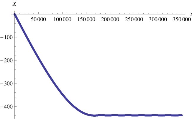
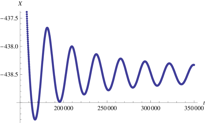
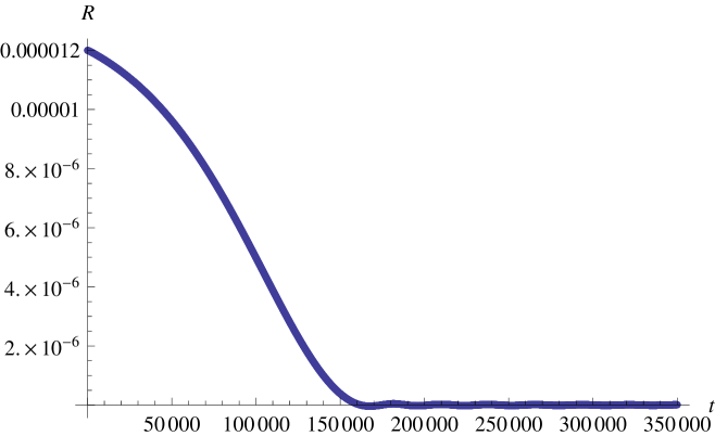
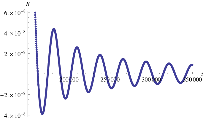
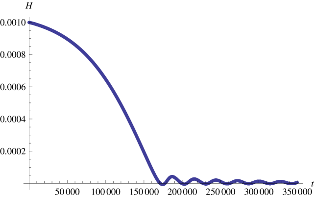
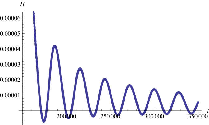
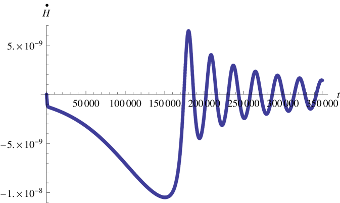
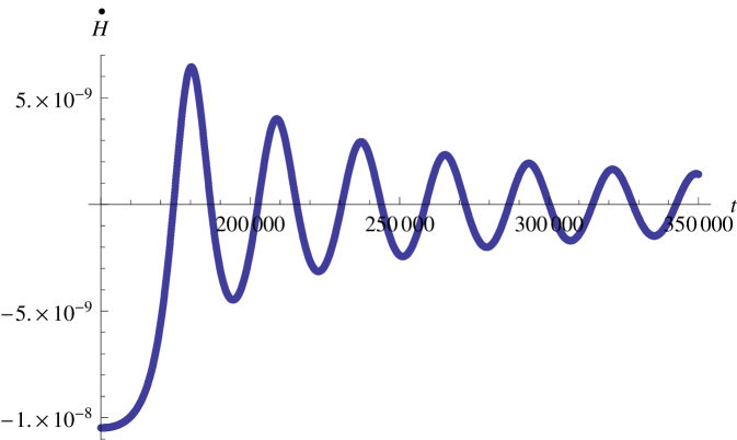
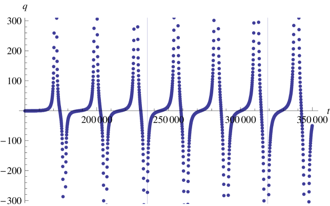
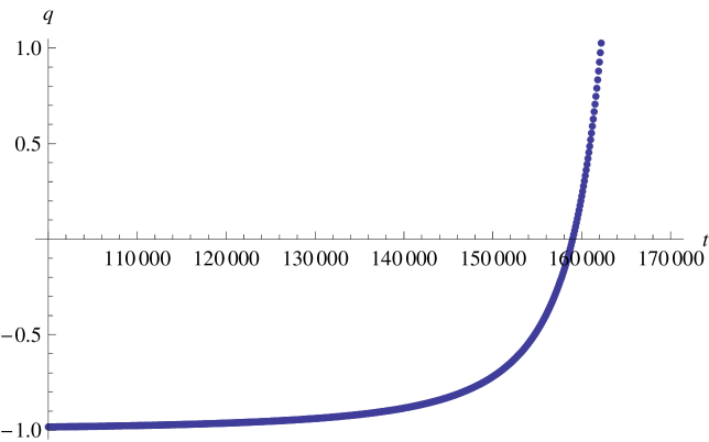
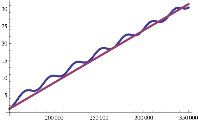
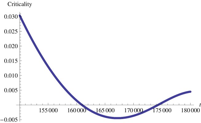
Our results are presented in the set of graphs that can be found in the very end. Some comments are in order:
$\bullet\;$ After the onset of and during the era of inflation, the source $X(t)$ grows while the curvature scalar $R(t)$ and Hubble parameter $H(t)$ decrease.
$\bullet\;$ Inflation ends and the time when this occurs is the time when the deceleration parameter $q(t)$ goes from negative to positive values.
$\bullet\;$ During the era of oscillations:
(i) The oscillations of $R(t)$ are centered around $R=0$, have an envelope behaving like $t^{-1}$ and a frequency $\omega$ in agreement with (67)
(ii) Although there is net expansion, the oscillations of $H(t)$ take it to small negative values for small time intervals. The presence of these short deflation periods is a novel feature of the model and may have consequences on the primordial perturbation spectrum.
(iii) The oscillations of $\dot{H}(t)$ show that there is almost no difference between $R(t)$ and $6\dot{H}$ and, therefore, the term in $R(t)$ proportional to $H^{2}(t)$ is insignificant during this era.
(iv) The oscillations of the scale factor $a(t)$ are centered around a linear increase with time.

It is important to note at this stage the excellent agreement of the analytical results derived in Section 4 with their numerical equivalents. The two basic parameters to concentrate are,
$\bullet\;$ Criticality: It occurs at step $i=160942$, as the detailed data of Figure 12 indicates, and at that point:

$$X[160942]\;=\;-438.50\qquad,\qquad q[160942]\;=\;0.50\;\;,$$ (68)

in complete agreement with the analytical predictions (66) and (91) respectively.
$\bullet$ Oscillation frequency: ¿From the detailed data of Figure 4 we conclude that six oscillations have occured between steps $i=174291$ and $i=342478$. Hence, we have:

$$T\;=\;\frac{342478-174291}{6}\,\Delta t\;=\;\frac{2\pi}{\omega}\qquad\Longrightarrow\qquad\omega\;=\;\frac{2.24\times 10^{-4}}{\Delta t}\;\;,$$ (69)

which compares very well with the analytical prediction (67).

4 Analytical Results

With the evolution equation (51) as a starting point, we can analytically derive some results for the physical system under study. Our ansatz restricts the function $f$ to be monotonically unbounded. Therefore, there exists a critical point $X_{cr}$ such that:

$$1\,-\,8\pi\epsilon\,f[-\epsilon\,X_{cr}]\;=\;0\qquad\Longrightarrow\qquad X_{cr}\;=\;-\,\frac{1}{\epsilon}\;f^{-1}\Big{(}\frac{1}{8\pi\epsilon}\Big{)}\;\;.$$ (70)

Inflationary evolution dominates roughly until we reach the critical point. Close to the critical point the induced pressure $p$ is small and, thus, it makes sense to expand $f$ around its critical point and use the resulting perturbation theory for the subsequent evolution:

$$2{\dot{H}}+3H^{2}\!\! = \!\!3H_{0}^{2}\,\Big{\{}\,1\,-\,8\pi\epsilon\,f[-\epsilon\,X_{cr}-\epsilon(X-X_{cr})]\,\Big{\}}$$ (71)

$$= \!\!3H_{0}^{2}\,\Bigg{\{}\,1\,-\,8\pi\epsilon\,\Big{(}\,f[-\epsilon\,X_{cr}]\,-\,\epsilon(X-X_{cr})\,f^{\prime}[-\epsilon\,X_{cr}]\,\Big{)}\qquad$$

$$\hskip 85.35826pt+\,O\Big{(}\epsilon^{2}(X-X_{cr})^{2}\Big{)}\;\Bigg{\}}$$

$$\simeq \!\!24\pi\epsilon^{2}\,H_{0}^{2}\,(X-X_{cr})\,f^{\prime}[-\epsilon\,X_{cr}]\;\;.$$

Neglecting all higher order terms is a superb approximation given the very small realistic values of $\epsilon$.

Moreover, using (28) we rewrite the co-moving time derivative of the Hubble parameter as:

$${\dot{H}}\;=\;\frac{1}{6}R\,-\,2H^{2}\;\;.$$ (72)

Consequently, the evolution equation (71) becomes:

$$-R\,+\,3H^{2}\;\simeq\;-72\pi\,(\epsilon H_{0})^{2}\,(X-X_{cr})\,f^{\prime}_{cr}\;\;,$$ (73)

where we have defined:

$$f^{\prime}_{cr}\;\equiv\;f^{\prime}[-\epsilon\,X_{cr}]\;\equiv\;-\frac{1}{\epsilon}\,\frac{d}{dX}f[-\epsilon\,X]\Big{|}_{X=X_{cr}}\;\;.$$ (74)

Action of the d’Alembertian operator (33) on (73) gives:

$$\ddot{R}\,+\,2H\,\dot{R}\,+\,(\omega^{2}-{\dot{H}})\,R\,+\,\Big{[}\,3H^{2}R-36H^{4}\,\Big{]}\;\simeq\;0\;\;,$$ (75)

with the understanding that:

$$\omega\;\equiv\;\epsilon H_{0}\,\sqrt{72\pi\,f^{\prime}_{cr}}\;\;.$$ (76)

It will turn out that the term in brackets is subdominant and we can focus our attention to the differential equation:

$$\ddot{R}\,+\,2H\,\dot{R}\,+\,\Big{(}\omega^{2}-{\dot{H}}\Big{)}\,R\;\simeq\;0\;\;,$$ (77)

which describes a damped oscillator. To solve the above equation we first scale out the Hubble friction term by defining:

$$R\;\equiv\;\frac{1}{a}\,S\;\;,$$ (78)

so that (77) becomes:

$$\ddot{S}\,+\,\Big{(}\omega^{2}-2{\dot{H}}-H^{2}\Big{)}\,S\;\simeq\;0\;\;,$$ (79)

and, in the large time limit, is solved by:

$$S(t)\;\simeq\;K_{1}\,\sin(\omega t+\varphi)\qquad,\qquad\omega^{2}\;\gg\;\Big{|}-2{\dot{H}}-H^{2}\Big{|}\;\;.$$ (80)

Hence, by using (78) and (28), we have:

$$K_{1}\,\sin(\omega t+\varphi)\;\simeq\;a\,R\;=\;6\,\frac{d}{dt}(Ha)\,+\,6H^{2}a\;\simeq\;6\,\frac{d}{dt}(Ha)\;\;.$$ (81)

¿From (81) we immediately conclude:

$${\dot{a}}(t)\!\! \simeq \!\!K_{2}\,-\,\frac{K_{1}}{6\,\omega}\,\cos(\omega t+\varphi)\;\;,$$ (82)

$$a(t)\!\! \simeq \!\!K_{3}\,+\,K_{2}\,t\,-\,\frac{K_{1}}{6\,\omega^{2}}\,\sin(\omega t+\varphi)\;\;.$$ (83)

and our large time results are:

$$\lim_{t\gg 1}\,H(t)\!\! \simeq \!\frac{1}{t}\,-\,\frac{K_{1}}{6K_{2}\,\omega}\,\frac{\cos(\omega t+\varphi)}{t}\,+\,O\Big{(}\frac{1}{t^{2}}\Big{)}\;\;,$$ (84)

$$\lim_{t\gg 1}\,{\dot{H}}(t)\!\! \simeq \!\frac{K_{1}}{6K_{2}}\,\frac{\sin(\omega t+\varphi)}{t}\,+\,O\Big{(}\frac{1}{t^{2}}\Big{)}\;\;,$$ (85)

$$\lim_{t\gg 1}\,R(t)\!\! \simeq \!\frac{K_{1}}{K_{2}}\,\frac{\sin(\omega t+\varphi)}{t}\,+\,O\Big{(}\frac{1}{t^{2}}\Big{)}\;\;.$$ (86)

¿From the asymptotic solution that we just obtained, the physical picture that emerges so far is that of a universe in which, as the exit from the inflationary era approaches, oscillations in $R$ become significant; their frequency $\omega$ is given by (76) and, according to (86), their envelope is linearly falling with time.

We can get further insight by computing the deceleration parameter $q$ at criticality. This is most easily done by considering the equations of motion (29-30) from which we deduce that:

$$-2{\dot{H}}\;=\;8\pi G\,(\rho+p)\;=\;\Lambda\,8\pi\epsilon\,\frac{\rho+p}{\Lambda^{2}}\;\;.$$ (87)

Then, we rewrite (29) in a form convenient for our purpose:

$$3H^{2}\!\! = \!\!\Lambda\,+\,8\pi G\,\rho$$ (88)

$$= \!\!\Lambda\,\Big{[}\,1\,+\,8\pi\epsilon\,\frac{\rho}{\Lambda^{2}}\,\Big{]}\;=\;\Lambda\,\Big{[}\,1\,-\,8\pi\epsilon\,\frac{p}{\Lambda^{2}}\,+\,8\pi\epsilon\,\frac{\rho+p}{\Lambda^{2}}\,\Big{]}\;\;,$$

and use (87-88) to express the decelaration parameter (20) in the following way:

$$q\;=\;-1\,-\,\frac{\dot{H}}{H^{2}}\;=\;-1\;+\;\frac{3}{2}\times\frac{\Lambda\,8\pi\epsilon\,\frac{\rho+p}{\Lambda^{2}}}{\Lambda\,\Big{[}\,1\,-\,8\pi\epsilon\,\frac{p}{\Lambda^{2}}\,+\,8\pi\epsilon\,\frac{\rho+p}{\Lambda^{2}}\,\Big{]}}\;\;.$$ (89)

The definitions (70) of criticality and (47) of pressure imply:

$$1\,-\,8\pi\epsilon\,f[-\epsilon\,X_{cr}]\;=\;1\,-\,8\pi\epsilon\,\frac{p_{cr}}{\Lambda^{2}}\;=\;0\;\;,$$ (90)

and allow us to conclude that:

$$q_{cr}\;=\;-1+\frac{3}{2}\;=\;+\,\frac{1}{2}\;\;$$ (91)

At the onset of inflation $q_{0}=-1$. Since by the time the universe arrived at the critical point the decelaration parameter had already reached positive values – $q_{cr}=+\frac{1}{2}$ – the epoch of inflation ended before the universe evolved to the critical time.

To investigate whether the dynamical system is underdamped at the critical point, we isolate all terms of the full equation (75) that affect the frequency:

$$frequency\;\;terms\qquad\Longrightarrow\qquad\Big{(}\,\omega^{2}-{\dot{H}}+3H^{2}\,\Big{)}\,R\;\;.$$ (92)

We have already seen that:

$$q_{cr}\;=\;-1\,-\,\frac{\dot{H}_{cr}}{H_{cr}^{2}}\;=\;+\,\frac{1}{2}\qquad\Longrightarrow\qquad-{\dot{H}}_{cr}\;=\;\frac{3}{2}\,H_{cr}^{2}\;\;,$$ (93)

leading to a positive frequency determining coefficient:

$$\Big{(}\,\omega^{2}-{\dot{H}}+3H^{2}\,\Big{)}\,\Big{|}_{cr}\;=\;\omega^{2}\,+\,\frac{9}{2}\,H_{cr}^{2}\,>\,0\;\;.$$ (94)

Hence, at criticality the system is underdamped implying again that oscillations start around the end of inflation.

It is also interesting to work out an approximate but direct relation between the frequency $\omega$ and the Hubble parameter $H$ at the critical time. The starting point is equation (87) and the approximation consists of evaluating its right hand side in de Sitter spacetime: