Boolean Network Approach to Negative Feedback Loops of the p53 Pathways: Synchronized Dynamics and Stochastic Limit Cycles

Abstract

Deterministic and stochastic Boolean network models are build for the dynamics of negative feedback loops of the p53 pathways. It is shown that the main function of the negative feedback in the p53 pathways is to keep p53 at a low steady state level, and each sequence of protein states in the negative feedback loops, is globally attracted to a closed cycle of the p53 dynamics after being perturbed by outside signal (e.g. DNA damage). Our theoretical and numerical studies show that both the biological stationary state and the biological oscillation after being perturbed are stable for a wide range of noise level. Applying the mathematical circulation theory of Markov chains, we investigate their stochastic synchronized dynamics and by comparing the network dynamics of the stochastic model with its corresponding deterministic network counterpart, a dominant circulation in the stochastic model is the natural generalization of the deterministic limit cycle in the deterministic system. Moreover, the period of the main peak in the power spectrum, which is in common use to characterize the synchronized dynamics, perfectly corresponds to the number of states in the main cycle with dominant circulation. Such a large separation in the magnitude of the circulations, between a dominant, main cycle and the rest, gives rise to the stochastic synchronization phenomenon.

KEY WORDS: Hopfield network; Stochastic Boolean network; Boltzmann machine; circulation; stochastic limit cycles; synchronization; p53 protein;

I Introduction

Thousands of papers have been reported in the field of p53 protein during the last three decades since 1979, including both the experimental and theoretical analysis. p53, the tumor suppressor, transcriptionally activates Mdm2, which in turn targets p53 for degradation (Piette et al. 1997, Prives et al. 1998, Vogelstein et al. 2000, Momand et al. 2000, Michael et al. 2003), keeping p53 at a low steady state level. The low steady state of p53 is essential for normal cell proliferation because p53 induces either cell cycle arrest or programmed cell death. The concentration of p53 increases in response to stress signals, such as DNA damage, inducing a transition to oscillations of p53 level. Following stress signal, p53 also activates transcription of several hundred genes, which are involved in the program of cell cycle arrest, apoptosis, cellular senescence and DNA repair. Therefore, it is important to note that many additional proteins interact with p53 and Mdm2, so that a number of positive and negative autoregulatory feedback loops acting upon the p53 response are embedded inside a network with a few additional interactions (Harris et al. 2005).

Several mathematical models have been proposed to explain the damped oscillations of p53, either in cell population or in a single-cell, most of which are deterministic model of ordinary differential equations (Mihalas et al. 2000, Lev Bar-Or et al. 2000, Monk et al. 2003, Ma et al. 2003, Ciliberto et al. 2005). On the other hand, the stochastic nature of p53 dynamics has also been observed and caused more and more interest nowadays (Ma et al. 2003).

However, in many cellular biochemical modelling, a detailed model, whether the deterministic one based on mass-action law, Michaelis-Menten kinetics and Hill function, or the stochastic molecular number-based CME(chemical master equation), is not warranted because of a lack of enough quantitative experimental data. Alternatively, one can develop discrete state network model, i.e., deterministic and stochastic Boolean networks, of a complex biological system using the available information on the activation and repression from one signaling molecules to another, e.g., the kind of signaling wiring diagram as the Fig. 1 in (Li et al. 2004), where Li et. al. have developed a discrete Boolean model by applying the approach of Hopfield for neural networks for yeast cell-cycle regulatory network with 11 nodes. The main results of (Li et al. 2004) are that the network is both dynamically and structurally stable. The biological steady state, known as the G1 phase of a cell cycle, is a global attractor of the dynamics; the biological pathway, i.e., the returning to G1 phase after perturbation, is a globally attracting dynamic trajectory. The deterministic Boolean model has been further extended to incorporate stochastic dynamics (Zhang et al.2006). They found that both the biological steady state and the biological pathway are well preserved under a wide range of noise level. Furthermore, recently we investigated the synchronized dynamics and nonequilibrium steady states in the stochastic yeast cell-cycle network (Ge et al. 2007), applying the mathematical circulation theory of Markov chains(Jiang et al. 2004).

In the present paper, deterministic and stochastic Boolean network models are build for the dynamics of negative feedback loops of the p53 pathways. It is shown that the main function of the negative feedback in the p53 pathways is to keep p53 at a low steady state level, and each sequence of protein states in the negative feedback loops, is globally attracted to a closed cycle of the p53 dynamics after being perturbed by outside signal (e.g. DNA damage). Our theoretical and numerical studies show that both the biological stationary state and the biological oscillation after being perturbed are stable for a wide range of noise level. Applying the mathematical circulation theory of Markov chains, we investigate their stochastic synchronized dynamics and by comparing the network dynamics of the stochastic model with its corresponding deterministic network counterpart, a dominant circulation in the stochastic model is seen to be the natural generalization of the deterministic limit cycle in the deterministic system.

It is shown that a large separation in the magnitude of the circulation, between a dominant main cycle and the rest, gives rise to the stochastic synchronization phenomenon and the stochastic global attractive behavior, and moreover the power spectrum of the trajectory has a main peak, whose period converges just to the number of states in the dominant cycle. Furthermore, the net circulation of the dominant cycle increases monotonically with the noise-strength parameter $\beta$, approaching its deterministic limit; while the circulation of all the other cycles approaches zero very fast when $\beta$ is quite large. Together, these observations provide a clear picture of the nature of the synchronization and stochastic limit cycles in a stochastic network in terms of the probabilistic circulation of NESS (nonequilibrium steady states) (Jiang et al. 2004).

For the completeness of the work, in supporting information, we give a theoretical sketch of some relevant results on biological networks, including a classification of the deterministic and stochastic Boolean networks and their correspondence. Also a short introduction of the mathematical theory of stochastic circulation for Markov chains is introduced and applied to deterministic and stochastic networks. It is shown that the stochastic Boolean network is reversible if and only if the matrix $T$ in the model is symmetric, and the net NESS circulation is strictly positive as long as the probability of the directed cycle is larger than that of its reversal.

II Boolean network approach

Since the influential work of J.J. Hopfield in 1980s’ (Hopfield 1982, Hopfield 1984), the deterministic Boolean (Hopfield) network has been applied to various fields of sciences. Amit (Amit 1989) has introduced a temperature-like parameter $\beta$ that characterizes the noise in the network and constructed a probabilistic Boolean network called Boltzmann machine. The deterministic and stochastic Boolean networks have found wide range of applications in biological networks.

In our model, the states of the nodes(proteins, DNAs or RNAs) in the network at the n-th step are represented by variables $X_{n}=(X_{n}^{1},X_{n}^{2},\cdots,X_{n}^{N})$ respectively, where $N$ is the number of nodes in the network. Each node $i$ has only two values, $X_{n}^{i}=1$ and $X_{n}^{i}=-1$, representing the active state and the reset state of this node respectively.

Deterministic Boolean network model:

The deterministic model consider in the present paper is a deformation of model $A1$ in supporting information. Let us suppose $N$ is a fixed integer, $S=\{1,2,\cdots,N\}$. We take the state space as $\{-1,1\}^{S}$. Denote the state of the $n$-th step as $X_{n}=(X_{n}^{1},X_{n}^{2},\cdots,X_{n}^{N})$, then the dynamic is as follows:

If $X_{n}\neq(-1,-1,\cdots,-1)$, then

$$X_{n+1}^{i}=\left\{\begin{array}[]{ll}\textrm{sign}(H_{i}),&\textrm{if}~{}\sum_{j=1}^{N}T_{ij}X_{n}^{j}\neq U_{i};\\ X_{n}^{i},&\textrm{if}~{}\sum_{j=1}^{N}T_{ij}X_{n}^{j}=U_{i};\end{array}\right.$$ (3)

where the function $\textrm{sign}(x)=\left\{\begin{array}[]{ll}1&x>0;\\ 0&x=0;\\ -1&x<0,\end{array}\right.$ $H_{i}=\sum_{j=1}^{N}T_{ij}X_{n}^{j}-U_{i}$ is the input to the i-th node and $U_{i}~{}(1\leq i\leq N)$, given a priori, are called the threshold of the $i$-th unit.

And if $X_{n}=(-1,-1,\cdots,-1)$, then $X_{n+1}=X_{n}$ when the parameter $\gamma=0$ representing that the system is under normal environment, and $X_{n+1}=(1,-1,-1,\cdots,-1)$ when the parameter $\gamma=1$ representing there are some perturbation(signal) of the system (e.g. DNA damage) emerge.

Stochastic Boolean Network model:

The stochastic model consider in the present paper is a deformation of model $C$ in supporting information, which is similar to the model in (Ge et al. 2007). Consider a Markov chain $\{X_{n}=(X_{n}^{1},X_{n}^{2},\cdots,X_{n}^{N}),n=0,1,2,\cdots\}$ on the state space $\{-1,1\}^{S}$, with transition probability given as follows:

$$P(X_{n+1}|X_{n})=\prod_{i=1}^{N}P_{i}(X_{n+1}^{i}|X_{n}),$$ (4)

where

$$P_{i}(X_{n+1}^{i}|X_{n})=\frac{\exp(\beta X_{n+1}^{i}H_{i})}{\exp(\beta H_{i})+\exp(-\beta H_{i})},$$

in which $H_{i}=\sum_{j=1}^{N}T_{ij}X_{n}^{j}-U_{i}$ is the input to the i-th node, if $\sum_{j=1}^{N}T_{ij}X_{n}^{j}\neq U_{i}$ and $X_{n}\neq(-1,-1,\cdots,-1)$ or $i\geq 2$,

$$P_{i}(X_{n+1}^{i}|X_{n})=\left\{\begin{array}[]{ll}\frac{1}{1+e^{-\alpha}},&X_{n+1}^{i}=X_{n}^{i};\\ \frac{e^{-\alpha}}{1+e^{-\alpha}},&X_{n+1}^{i}=1-X_{n}^{i},\end{array}\right.$$

if $\sum_{j=1}^{N}T_{ij}X_{n}^{j}=U_{i}$ and $X_{n}\neq(-1,-1,\cdots,-1)$ or $i\geq 2$, and

$$P_{1}(X_{n+1}^{i}|X_{n})=\left\{\begin{array}[]{ll}1-\gamma,&X_{n+1}^{i}=X_{n}^{i},\\ \gamma,&X_{n+1}^{i}=1-X_{n}^{i},\end{array}\right.$$

if $X_{n}=(-1,-1,\cdots,-1)$, where the parameter $0\leq\gamma\leq 1$ still represents the stochastic perturbations of the system from extracellular environment.

In the above equation, $\alpha(>0)$, $\beta(>0)$, $T_{ij}$ and $U_{i}~{}(1\leq i,j\leq N)$ are parameters of the model. The positive temperature-like parameter $\beta$ represents noise in the system from the perspective of statistical physics (Amit 1989, Zhang et al. 2006). Noticeably, the actual noises within a cell might not be constant everywhere, but here we use a system-wide noise measure for simplicity. To characterize the stochasticity when the input $H_{i}$ to a node is zero, we have to introduce another parameter $\alpha$. This parameter controls the likelihood for a protein to maintain its state when there is no input to it.

The previous parameters $\beta$ and $\alpha$ represent the intracellular noise due to thermodynamic fluctuations, and on the other hand, we need another parameter $\gamma$ to characterize the extracellular signal strength with appropriate stochasticity. Since the signal is not purely disordered, we can not express the probability $P_{1}(X_{n+1}^{i}|X_{n})$ when $X_{n}=(-1,-1,\cdots,-1)$ as the exponential form analogous to the Boltzmann distribution, hence we directly regard $\gamma$ as the probability transiting from $(-1,-1,\cdots,-1)$ to $(1,-1,\cdots,-1)$.

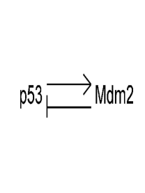
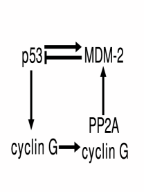
In our models below, $T_{ij}=1$ for a arrow from protein $j$ to protein $i$, and $T_{ij}=-1$ for a horizontal bar instead of arrowhead from protein $j$ to protein $i$(Fig. 1, 2). And it is indispensable to point out that self-connections haven’t been taken into consideration in our models for simplicity.

Similar to Proposition II.6 in supporting information, with the same initial distribution, when $\gamma\rightarrow 0$, and $\alpha$, $\beta\rightarrow\infty$, then the stochastic Boolean network model converges to the corresponding deterministic Boolean network model with parameter $\gamma=0$; and when $\gamma\rightarrow 1$, and $\alpha$, $\beta\rightarrow\infty$, then the stochastic Boolean network model converges to the corresponding deterministic Boolean network model with parameter $\gamma=1$.

III Steady states and synchronized dynamics of the p53 pathways

From biochemical perspective, the microscopic variables for a cellular regulatory network are the concentrations, or numbers, of various mRNAs, regulatory proteins, and cofactors. If all the biochemistry were known, then the dynamics of such a network would be represented by a chemical master equation (McQuarrie 1967, Gillespie 1977). Unfortunately, much of the required information is not available, nor such a “fully-detailed” model will always be useful. Phenomenologically the concentrations of key players of a biochemical regulatory network can often be reduced to two or three states, such as resting state, activated state, inactivated state, etc. (Fall et al. 2002). The interactions between these states are usually determined from experimental data.

The present study will build simple deterministic and stochastic Boolean network models for several negative feedback loops of the p53 pathways, and more important, provides a sound mathematical explanation of the synchronized dynamics and stochastic limit cycles in the stochastic Boolean network model after being perturbed by stress signals, in terms of the theory of nonequilibrium circulations (Jiang et al. 2004). This makes the description of pathway more definite and penetrating.

III.1 The core regulation

Negative feedback loops, composed of one transcription arm and one protein-interaction arm, are a common network motif across organisms. p53, the tumor suppressor, transcriptionally activates Mdm2, which in turn targets p53 for degradation. Although it is believed that the existence of negative feedback loop in biological systems can always gives rise to oscillations, yet it is not sufficient for the appearing of a limit cycle in the deterministic ODE model from the mathematical point of view.

A bit out of expectation is, if we use the deterministic Boolean network even to the simplest case(Fig.1), the existence of negative feedback already gives rise to a limit cycle corresponding to oscillations in a biological system, when there exists the outside signal (i.e. $\gamma=1$).

Model: From Section II(For Fig.1).

The first node $X_{n}^{1}$: p53; and the second node $X_{n}^{2}$: Mdm2.

$N=2$ is the number of nodes in the model. For simplicity, we set thresholds as $U_{1}=U_{2}=0$. And the interacting matrix

$$T=\left[\begin{array}[]{ll}0&-1\\ 1&0\end{array}\right]$$

The deterministic model with $\gamma=0$ has a global attractor $(-1,-1)$, which corresponds to the fact that the main function of the negative feedback between $p53$ and $Mdm2$ is to keep $p53$ at a low steady state level in normal cells.

On the other hand when $\gamma=1$, the deterministic model has a unique limit cycle consist of $4$ state, which is described by Table 1. It corresponds to the fact that the stress signal (e.g. DNA damage) will activate the protein p53(i.e. time-2 point in Table 1) and induce a transition to oscillations of p53 level after being perturbed from the outside environment.

Time	p53	Mdm2
1	1	-1
2	1	1
3	-1	1
4	-1	-1

Table 1: Cycle evolution of the protein states in the negative feedback loop of p53 and Mdm2 after being perturbed.

Moreover, as long as the stress signal strength $\gamma$ is sufficiently low $(0<\gamma<<1)$ or sufficiently high $(0<1-\gamma<<1)$, the stochastic Boolean network model would preserve the dynamics of the corresponding deterministic model at a certain low level of noise. As it illustrates the same phenomenon as the Cyclin G/Mdm-2 loop given below, so we won’t show the data here.

Similar model can also be built and analyzed exactly by the same reasoning, to other ubiquitin ligases that promote p53 ubiquitination and subsequent proteasomal degradation (Fig. 10 in Harris et al. 2005). We only use the simplest example as a start, and pass directly to a really delicate interesting case.

III.2 Cyclin G/Mdm2 loop

Model: From Section II.

The first node $X_{n}^{1}$: p53; The second node $X_{n}^{2}$: cyclin G; The third node $X_{n}^{3}$: PP2A cyclin G; The last node $X_{n}^{4}$: Mdm-2.

N=4 is the number of nodes in the model. For simplicity, we set thresholds as $U_{1}=U_{2}=U_{3}=U_{4}=0$. And from Fig.2, the interacting matrix

$$T=\left[\begin{array}[]{llll}0&0&0&-1\\ 1&0&0&0\\ 0&1&0&0\\ 1&0&1&0\end{array}\right].$$

The deterministic model with $\gamma=0$ has a global attractor $(-1,-1,-1,-1)$, which corresponds to the fact that $p53$ is kept at a low steady state level in normal cells.

On the other hand, the deterministic model when $\gamma=1$ has a unique limit cycle consist of $8$ state, which is described by Table 2. It corresponds to the fact that the stress signal (e.g. DNA damage) will activate the protein p53(i.e. time-2 point in Table 2) and induce a transition to oscillations of p53 level after being perturbed from the outside environment, which roughly corresponds to the p53 pathway or biological trajectory described in (Harris et al. 2005) “One of the most active of the p53-responsive genes is the cyclin G gene. It is rapidly transcribed to high levels after p53 activation in a wide variety of cell types.”(i.e. Time-3 point in Table 2) “The cyclin G protein makes a complex with the PP2A phosphatase, which removes a phosphate residue from Mdm-2, which is added to the Mdm-2 protein by a cdk kinase” (i.e. Time-4,5 points in Table 2). Our language in the present paper is more definite and penetrating than the quotations.

Time	p53	Cyclin G	PP2A Cyclin G	Mdm-2
1	(-1	-1	-1	-1)
2	(1	-1	-1	-1)
3	(1	1	-1	-1)
4	(1	1	1	-1)
5	(1	1	1	1)
6	(-1	1	1	1)
7	(-1	-1	1	1)
8	(-1	-1	-1	1)

Table 2: Cycle evolution of the protein states in the Cyclin G/Mdm-2 loop after being perturbed.

Numerical Simulation of the stochastic Boolean network model

The numerical results about the cyclic motion of this stochastic model are quite similar to the stochastic Boolean network model of the cell-cycle, which we have recently discussed (Ge et al. 2007). The main conclusion is that, given the structure of the negative feedback present in Fig. 2, the stochastic model still exhibits well pronounced oscillations after being seriously perturbed, which is excellently characterized by the circulation theory introduced in the supporting information.

Numerical computations for the current model(Fig.2), are carried out with the famous Gillespie’s method (Gillespie 1977) of the stochastic Boolean network model using MATLAB, and the results are given in the following figures. The network with $4$ binary nodes has a total of $2^{4}=16$ number of states. Here, we can present the dynamics of the network in terms of the integer states $0,1,2,\cdots,2^{4}-1=15$ on a line. This 1-d system is reversible if and only if the 4-d system is reversible.

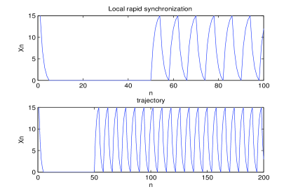
Fig. 3 are the basic behavior of a random trajectory. The upper panel shows that there arises the phenomenon of local rapid synchronization like that observed in (Hopfield 1995) during a very short time period after the value of $\gamma$ transits from $0.01$ to $0.99$ at time $n=50$, when $\beta$ and $\alpha$ are sufficiently large. The lower panel is a random trajectory over a longer time. Little deviation is shown from the deterministic trajectory in Table 2 after being perturbed at time $n=50$, which implies that the stochastic model still leads to well pronounced oscillations when the perturbation from the environment is sufficiently high.

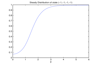
Fig. 4 shows the stationary distribution of the state $(-1,-1,-1,-1)$ in the stochastic model which increasingly approaches $1$ when $\beta$ tends to infinity. This excellently corresponds well to the dynamics of the deterministic model when $\gamma=0$. At large $\beta$ (low temperature or small noise level), the low level state $(-1,-1,-1,-1)$ is the most probable state of the system. So analogous to the concept of the deterministic model, this state $(-1,-1,-1,-1)$ can be regarded as the global attractor of the stochastic model. Moreover, one observes a phase-transition like behavior of the stationary distribution of the state $(-1,-1,-1,-1)$ while varying the noise level $\beta$ (similar behavior has been seen in (Qu et al. 2002)).

Then we turn to investigate the synchronized dynamics when the signal parameter $\gamma$ is sufficiently high(i.e. $0<1-\gamma<<1$). The keys to understand synchronization behavior in stochastic Boolean network models are ($i$) establishing a correspondence between a stochastic dynamics and its deterministic counterpart; and ($ii$) identifying the cyclic motion in the stochastic models.

As there is a growing awareness and interest in studying the effects of noise in biological networks, it becomes more and more important to quantitatively characterize the synchronized dynamics mathematically in stochastic models, because the concepts of limit cycle and fixed phase difference no longer holds in this case. Instead, physicists and biologists always have to characterize synchronized dynamics by the distinct peak of some spectrum or just only by observing the stochastic trajectories, which however may cause ambiguities in the conclusion. Therefore, a logical generalization of limit cycle to the stochastic model is well worth to be developed.

In case of the stochastic models of biological networks, there does exist a rather complete mathematical theory for the cyclic motion of the corresponding Markov chains, which has been developed for more than twenty years (Jiang et al. 2004, Kalpazidou 1995). One of the most important concepts in this mathematical theory of NESS is the circulation, which corresponds to the cycle kinetics in open chemical systems (Hill 1989, Qian 2005). The details of mathematical theory is supplied in the supporting information.

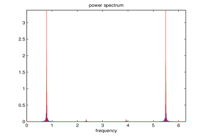
To further characterize the synchronized dynamics, we give Fig. 5 which shows the Fourier power spectrum of the stochastic trajectory with different values of $\beta$ respectively. Using MATLAB, the discrete Fourier transform for time series $\{x_{1},x_{2},\cdots,x_{n}\}$ is defined as

$$y_{m}=\left|\sum_{k=1}^{n}x_{k}e^{-i(2\pi/n)(m-1)(k-1)}\right|,\hskip 11.38092pt\left(\frac{m-1}{n}2\pi,\ 1\leq m\leq n\right).$$ (5)

Therefore, by the Herglotz theorem (Qian et al. 1997 p. 331), the power spectrum of discrete trajectory has a symmetry $y_{m}=y_{n+2-m}$. For different sets of parameters, we found all the calculations give the same outstanding main peak in the Fig. 5. It is important to mention here that by ergodicity, different trajectories give the same power spectrum for any $\beta$ that is sufficiently large.

The single dominant peak in Fig. 5 implies there exists a global synchronization and a globally attractive phenomenon. Note that by representating our maps, one-to-one, from the $N$ binary nodes to the integers $0-15$, the synchronized behavior is preserved. It is possible that the map will cause some distortion in the power spectrum.

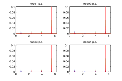
To further illustrate the synchronized behavior, Fig. 6 shows the power spectra of all the 4 individual nodes in the network. While subtle details are different, all exhibit the dominant peak, similar to that of the overall dynamics. This demonstrates further that synchronized dynamics is presented in the network.

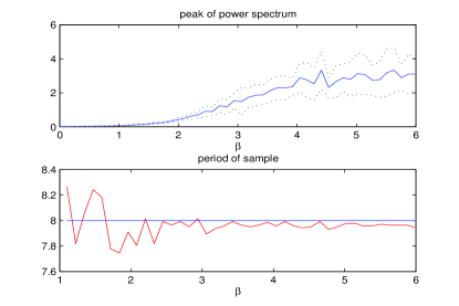
Fig. 7 plots the magnitude and the period of the dominant peak of the power spectrum in Fig. 5 respectively, as functions of the noise strength, i.e., the parameter $\beta$. It shows, as we have predicted, that the period converges to 8 which corresponds perfectly to the number of states in the main cycle of Table 2 when $\beta$ is large. We also put error bars on the upper panel of Fig. 7 with various values of $\beta$.

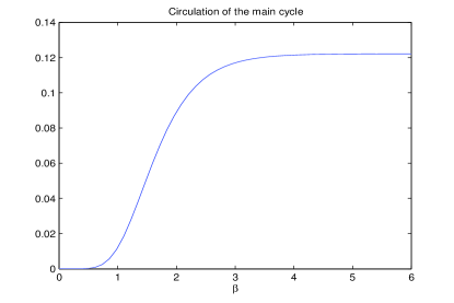
Finally, Fig. 8 shows how the net circulation of the dominant, main cycle varies with $\beta$, applying the determinant presentation of circulations according to Theorem II.4 in the supporting information. Note that circulation is just the time-averaged number of appearance of certain cycle along the stochastic trajectory of our model, and net circulation is just the difference between the circulations along the positive direction and negative direction of a specific cycle. It is clearly seen that the net circulation of the main cycle increases monotonically to $\frac{1}{8}$ that is just the reciprocal of the number of states in the main cycle, which implies the appearing of more and more distinct synchronization and global attractive behavior with increasing $\beta$. The direction of the net circulation does not change. It is also found that the circulation of negative direction along the main cycle is always quite low compared to the circulation of positive direction.

The net circulations of all the cycles are very small when $\beta$ and $\alpha$ are near zero, since the system is close to equilibrium(reversible) state when $\alpha=\beta=0$ according to lemma II.9 in supporting information.

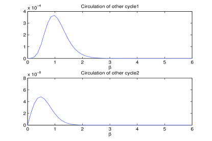
For large $\beta$, the net circulations of all the cycles except the main cycle are also very small by numerical simulation using the determinant expression in Theorem II.4 of supporting information. All the circulations of non-main cycles actually decrease with increasing $\beta$ when $\beta$ is large. Examples are shown in Fig. 9. This large separation in the magnitudes of the weights gives rise to the stochastic synchronization, and this stochastic limit cycle can be defined as a “stable” one, whose attractive domain is global.

As in (Zhang et al. 2006, Ge et al. 2007), we also notice that there exists an inflection point in the curve in Fig. 8. This implies a cooperative transition of the net circulation of the main cycle while varying the noise level $\beta$, which equivalently means some sort of “phase transition” around $\beta=2$ from chaotic fluctuations(period=infinity) at small $\beta$ to periodic fluctuations (period=8) at large $\beta$. Certainly, the implication of this observation remains to be further elucidated.

IV Discussion

From detailed models to simplified Boolean network approach

Deterministic nonlinear mathematical models, based on the Law of Mass Action, have been traditionally used for biochemical reaction networks. Furthermore, noises are unavoidable in small biochemical reaction systems such as those inside a single cell. Stochastic models with chemical master equations (CME) (McQuarrie 1967, Van Kampen 1981) should be developed, which has already provided important insights and quantitative characterizations in some cases of the biochemical system (Fox et al. 1994, Fox 1997, Zhou et al. 2005). Ref. (Wilkinson 2006) is a good introduction to the stochastic modelling in biology.

In many cellular biochemical modelling, it is impossible to build a detailed, molecular number-based CME model due to a lack of quantitative experimental data. Thus, one often seeks a simplified network model based on simple binary states of the signaling molecules. This leads to the Boolean, Markov network model of the p53 pathways we studied in the present paper.

Modelling the oscillatory dynamics of p53 pathways after being perturbed

The realization that p53 is a common denominator in human cancer has stimulated an avalanche of research since 1989. The p53 gene can integrate numerous signals that control cell life and death, and damped oscillations for p53 and Mdm2 has been observed and modeled (Lev Bar-Or et al. 2000, Ma et al. 2003). The Boolean network models built in the present paper, which omit some parameters to represent the degradation of the p53 protein in cells, only try to explain the mechanism of the oscillatory behavior of the p53 dynamics after being perturbed by stress signals rather than exhibiting the damped oscillations. The signal parameter $\gamma$ plays a very important role in the model similar to the cell cycle model in (Ge et al. 2007), which can induce the level of p53 from a low steady state to oscillated behaviors.

On the other hand, ideally, one should try to combine these Boolean network models of negative feedback loops together to construct a clear and integrated picture of the p53 pathways, maybe especially including several positive feedback loops (Harris et al. 2005). But unfortunately we haven’t developed a reasonable way to do so.

Synchronization and circulation in stochastic Boolean network

Synchronization is an important characteristics of many biological networks (Strogatz 2003, Winfree 2000) whose dynamics has been modelled traditionally by deterministic, coupled nonlinear ordinary differential equations in terms of regulatory mechanisms and kinetic parameters (Murray 2002, Fall et al. 2002). Two important classes of biological networks which have attracted wide attentions in recent years are neural networks (Scott 2002) and cellular biochemical networks (Goldbeter 1996).

As we know, the occurrence of a deterministic limit cycle in an ODE model is the hallmark of a synchronization phenomenon, while such a definite concept no longer holds in a stochastic system. It is observed that in our present model of p53 pathways, the trajectory concentrates around a main cycle, which we call stochastic limit cycle and is very similar to in many aspects the limit cycle of a deterministic model. Furthermore, the present work shows that the circulation in an irreversible Markov chain (Jiang et al. 2004) is a reasonable generalization of the concept of deterministic limit cycles, and provides a sound mathematical explanation of the synchronization in the stochastic Boolean network model.

Stability and robustness of the p53 genetic networks

Biological functions in living cells are controlled by protein interaction and genetic networks, and have to be robust to function in complex (and noisy) environments. More robustness would also mean being more evolvable, and thus more likely to survive.

More precisely, these molecular networks should be dynamically stable against various fluctuations which are inevitable in the living world. Therefore, the stability and robustness of Boolean network model can not be determined if the noise hasn’t been introduced into the model, since it is not reasonable to simply apply the Euclidean topology in mathematics to such a real biological discrete model not to say the magnitudes of the different attractive basins of fixed states and limit cycles as in the deterministic models. For instance, the recent analysis of stochastic cell-cycle Boolean networks (Ge et al. 2007, Zhang et al. 2006) just claimed the stability and robustness of the previous deterministic model (Li et al. 2004), in which Li, et.al. announced but didn’t really investigate the robustness of this model against perturbation. Hence, the numerical and theoretical studies in the present paper in some sense excellently exhibit the stability and robustness of the p53 genetic networks.

Figure 1: Negative feedback loop of p53 and Mdm2. Arrows denote stimulatory interactions, whereas horizontal bars instead of arrowheads indicate inhibitory influences.

Figure 2: Cyclin G/Mdm2 loop, redrawn from (Fig. 8 in Harris et al. 2005).

Figure 3: Stochastic trajectory and synchronization of the Cyclin G/Mdm-2 loop. Simulations are carried out with the parameters $\alpha=5$, $\beta=5$ and the values of $\gamma$ transits from $0.001$ to $0.999$ at time $n=50$.

Figure 4: Stationary distribution of the state $(-1,-1,-1,-1)$ in the stochastic model. Simulations are carried out with the parameters $\alpha=5$ and $\gamma=0.001$.

Figure 5: Power spectrum of the overall trajectory in the Cyclin G/Mdm-2 loop with the parameter $\alpha=5$ and $\gamma=0.999$ fixed, and with different $\beta$: blue: $\beta$=2.4; green: $\beta$=4.8; red: $\beta=6$. The discrete Fourier transform causes an alias; hence the spectrum is symmetric with respect to $\pi$ on the $[0,2\pi]$ interval.

Figure 6: Power spectra of individual nodes in the Cyclin G/Mdm-2 loop show a synchronization among all the nodes with the parameter $\alpha=5$ and $\gamma=0.999$ fixed, and different $\beta$: blue: $\beta$=2.4; green: $\beta$=4.8; red: $\beta$=6.

Figure 7: Magnitude and period of the dominant power-spectral peak as functions of $\beta$ in the Cyclin G/Mdm-2 loop, with $\alpha=5$ and $\gamma=0.999$. In the upper panel, the magnitude of the dominant power-spectral peak is averaged over 20 simulations. The solid curve is the mean, and the dotted curves are the mean $\pm$ standard deviation. The period approaches to 6 (the horizonal line) with increasing $\beta$.

Figure 8: Net circulation of the main cycle in the Cyclin G/Mdm-2 loop as a function of the noise strength, $\beta$, with the parameter $\alpha=5$ and $\gamma=0.999$ fixed.

Figure 9: Net circulation of several other cycles in the Cyclin G/Mdm-2 loop as a function of the noise strength, $\beta$, with the parameter $\alpha=5$ and $\gamma=0.999$ fixed.

References

- [1] Amit, D.J. 1989: Modeling brain function: The world of attractor neural networks. Cambridge University Press
- [2] Chen, Y., Chen, X. and Qian, M.P. 2006: Green-Kubo formula, autocorrelation function and fluctuation spectrum for finite Markov chains with continuous time. J. Phys. A: Math. Gen. 39 2539-2550
- [3] Ciliberto, A., Novak, B. and Tyson, J. 2005: Steady states and oscillations in the p53/Mdm2 network. Cell Cycle 4, 488–493
- [4] Fall, C.P., Marland, E.S., Wagner, J.M. and Tyson, J.J. 2002: Computational cell biology. New York: Springer-Verlag
- [5] Fox, R.F. and Lu, Y. 1994: Emergent collective behavior in large numbers of globally coupked independently stochastic ion channels. Phys. Rev. E 49(4) 3421-3431
- [6] Fox, R.F. 1997: Stochastic versions of the Hodgkin-Huxley equations. Biophys. J. 72 2068-2074
- [7] Ge, H., Qian, H. and Qian, M. 2008: Synchronized dynamics and nonequilibrium steady states in a yeast cell-cycle network. Math. Biosci. 211 132–152
- [8] Gillespie, D.T. 1977: Exact stochastic simulation of coupled chemical reactions. J. Phys. Chem. 81(25), 2340–2361
- [9] Goldbeter, A. 1996: Biochemical Oscillations and Cellular Rhythms: the Molecular Bases of Periodic and Chaotic Behaviour, New York: Cambridge Univ. Press
- [10] Harris, S.L. and Levine, A.J. 2005: The p53 pathway: positive and negative feedback loops. (Oncogene (24). 2899-2908)
- [11] Hill, T.L. 1989: Free Energy Transduction and Biochemical Cycle Kinetics. New York: Springer-Verlag
- [12] Hopfield, J.J. 1982: Neural networks and physical systems with emergent collective computational abilities. Proc. Natl. Acad. Sci. (79) 2554-2558
- [13] Hopfield, J.J. 1984: Neurons with graded response have collective computational properties like those of two-state neurons. Proc. Natl. Acad. Sci. (81) 3088-3092
- [14] Hopfield, J.J. 1995: Rapid local synchronization of action potentials: Toward computation with coupled integrate-and-fire neurons. Proc. Natl. Acad. Sci. (92) 6655-6662
- [15] Jiang, D.Q., Qian, M. and Qian, M.P. 2004: Mathematical theory of nonequilibrium steady states - On the frontier of probability and dynamical systems. (Lect. Notes Math. 1833) Berlin: Springer-Verlag
- [16] Jiang, D.Q. and Zhang, F.X. 2003: The Green-Kubo formula and power spectrum of reversible Markoc processes. J. Math. Phys. 44(10), 4681–4689
- [17] Kalpazidou, S.L. 1995: Cycle representations of Markov processes. (Applications of Mathematics. 28) Berlin: Springer-Verlag
- [18] Lev Bar-Or, R., Maya, R., Segel, L.A., Alon, U., Levine, A.J. and Oren, M. 2000: Generation of oscillations by the p53-Mdn2 feedback loop: a theoretical and experimental study. Proc.Natl.Acad.Sci. USA 97, 11250–11255
- [19] Li, F., Long, T., Lu, Y., et al. 2004: The yeast cell-cycle network is robustly designed. Proc. Natl. Acad. Sci. 101 (14) 4781-4786
- [20] Ma, L., Wagner, J., Rice, J.J., Hu, W., Levine, A.J. and Stolovitzky, G.A. 2003: A plausible model for the digital response of p53 to DNA damage. Proc. Natl. Acad. Sci. USA 102, 14266–14271
- [21] McQuarrie, D.A. 1967: Stochastic approach to chemical kinetics. J.Appl.Prob. 4(3), 413-478
- [22] Michael, D. and Oren, M. 2003: The p53-Mdm2 module and the ubiquitin system. Semin. Cancer Biol. 13, 49–58
- [23] Mihalas, G.L., Simon, Z., Balea, G. and Popa, E. 2000: Possible oscillatory behavior in p53-Mdm2 interaction computer simulation. J.Biol.Syst. 8, 21–29
- [24] Momand, J., Wu, H.H. and Dasgupta, G. 2000: Mdm2-master regulator of the p53 tumor suppressor protein. Gene 242, 15–29
- [25] Monk, N.A. 2003: Oscillatory expression of Hes1, p53, and NF-kappaB driven by transcriptional time delays. Curr. Biol. 13, 1409–1413
- [26] Murray, J.D 2002: Mathematical biology, 3rd Ed. New York: Springer 2002
- [27] Piette, J., Neel, H. and Marechal, V. 1997: Mdm2: keeping p53 under control. Oncogene 15, 1001–1010
- [28] Prives, C. 1998: Signaling to p53: breaking the Mdm2-p53 circuit. Cell 95, 5–8
- [29] Qian, H. 2005: Cycle kinetics, steady-state thermodynamics and motors–a paradigm for living matter physics. J. Phys. Cond. Matt. 17, S3783-S3794
- [30] Qian, M.P. and Gong, G.L. 1997: Stochastic Processes(second edition). Peking University Press. (in Chinese)
- [31] Qian, M.P. and Qian, M. 1982: Circulation for recurrent Markov chains. Z. Wahrsch. Verw. Gebiete 59, 203–210 (1982)
- [32] Qian, M.P., Qian, C. and Qian, M. 1984: Circulations of Markov chains with continuous time and the probability interpretation of some determinants. Sci. Sinica (Series A) 27(5), 470–481
- [33] Qu, X., Aldana, M. and Kadanoff, L.P. 2002: Numerical and theoretical studies of noise effects in the kauffman model. J. Statist. Phys. 109(5-6), 967–986
- [34] Scott, A.C. 2002: Neuroscience: A Mathematical Primer. New York: Springer-Verlag
- [35] Strogatz, S. 2003: Sync: The Emerging Science of Spontaneous Order. New York:Hyperion
- [36] Van Kampen N.G. 1981: Stochastic Processes in Physics and Chemistry. Amsterdam:North-Holland
- [37] Vogelstein, B., Lane, D. and Levine, A.J. 2000: Surfing the p53 network. Nature 408, 307–310
- [38] Wilkinson, D.J. 2006: Stochastic Modelling for Systems Biology. Chapman and Hall/CRC
- [39] Winfree, A.T. 2000: The Geometry of Biological Time, 2nd. Ed. Berline: Springer-Verlag
- [40] Zhou, T.S., Chen, L.N., and Wang, R.Q. 2005: A mechanism of synchronization in interacting multi-cell genetic systems. Physica D 211, 107–127
- [41] Zhang, Y., Qian, M.P., Ouyang, Q., et al. 2006: Stochastic model of yeast cell-cycle network. Physica D 219, 35–39