Sensitivity Amplification in the Phosphorylation-Dephosphorylation Cycle:
Nonequilibrium steady states, chemical master equation and temporal cooperativity

Abstract

A new type of cooperativity termed temporal cooperativity [Biophys. Chem. 105 585-593 (2003), Annu. Rev. Phys. Chem. 58 113-142 (2007)], emerges in the signal transduction module of phosphorylation-dephosphorylation cycle (PdPC). It utilizes multiple kinetic cycles in time, in contrast to allosteric cooperativity that utilizes multiple subunits in a protein. In the present paper, we thoroughly investigate both the deterministic (microscopic) and stochastic (mesoscopic) models, and focus on the identification of the source of temporal cooperativity via comparing with allosteric cooperativity.

A thermodynamic analysis confirms again the claim that the chemical equilibrium state exists if and only if the phosphorylation potential $\triangle G=0$, in which case the amplification of sensitivity is completely abolished. Then we provide comprehensive theoretical and numerical analysis with the first-order and zero-order assumptions in phosphorylation-dephosphorylation cycle respectively. Furthermore, it is interestingly found that the underlying mathematics of temporal cooperativity and allosteric cooperativity are equivalent, and both of them can be expressed by “dissociation constants”, which also characterizes the essential differences between the simple and ultrasensitive PdPC switches. Nevertheless, the degree of allosteric cooperativity is restricted by the total number of sites in a single enzyme molecule which can not be freely regulated, while temporal cooperativity is only restricted by the total number of molecules of the target protein which can be regulated in a wide range and gives rise to the ultrasensitivity phenomenon.

KEY WORDS: Phosphorylation-dephosphorylation cycle; Nonequilibrium steady states; Chemical master equation; Temporal cooperativity; Allosteric cooperativity; Ultrasensitivity

1 Introduction

Biological signal transduction processes are increasingly understood in quantitative terms, such that the switching of enzymes and proteins between phosphorylated and dephosphorylated states becomes a universal module [1, 2]. The biological activity of a target protein is often wakened by the phosphorylation reaction catalyzed by a specific kinase, and restrained by the dephosphorylation reaction catalyzed by a specific phosphatase, which is quite similar to the turning on and off procedure of an ordinary switch.

One of the key concepts in PdPC signaling is the switching sensitivity: the sharpness of the activation of the substrate protein in response to the concentration of the kinase is basic in the perspective of metabolic control analysis, usually termed as Hill coefficient first proposed by A. V. Hill [3].

Actually, the research about the sensitivity of single-enzyme catalysis activity, also known as the allosteric cooperativity, has already been developed for about forty years, since the classic paper of Monod, Wyman and Changeux [4] and Koshland, Nemethy and Filmer [5]. It is found in experiments that very few individual enzymes show positive cooperativity with Hill coefficient greater than $4$.

However, in the case of multi-enzyme systems such as the phosphorylation-dephosphorylation module, the situation is quite different. In the early 1980s, Goldbeter and Koshland [6, 7] discovered the ultrasensitivity phenomenon of a PdPC switch in terms of the zeroth order kinetics of kinase and phosphatase, where the Hill coefficient can be extremely high. Moreover, it has already been observed in experiments [8].

Recently, Qian [9, 10] has further elucidated the importance of open-system chemical reaction in terms of continuous ATP hydrolysis. It was found that the thermodynamic energy aspect of the signal transduction plays an important role in further understanding the function of PdPC switches, which confirms the well-known belief that signal transduction in biological systems actually consumes energy [11].

Most of the previous models [12, 6, 9, 13] built for the phosphorylation and dephosphorylation module were traditionally based on deterministic, coupled nonlinear ordinary differential equations in terms of regulatory mechanisms and kinetic parameters, which are widely used in the field of computational biology [14, 15]. Nowadays, as there is a growing awareness of the basic character of noise in the study of the effects of noise in biological networks, it becomes more and more important to develop stochastic models with chemical master equations (CME) based on biochemical reaction stoichiometry, molecular numbers, and kinetic rate constants. Such an approach has already provided important insights and quantitative characterizations of a wide range of biochemical systems [16, 17, 18, 19, 20, 21, 22, 23], especially in recent studies on gene expression [24, 25].

On the other hand, these stochastic models for systems cell biology would exhibit nonequilibrium steady states (NESS), in which their mesoscopic properties can be rigorously investigated from the trajectory point of view [26, 27, 28]. Moreover, several recently interesting experimental results can only be explained by stochastic models [29].

The aim of this paper is to thoroughly investigate temporal cooperativity [9] emerged in the signal transduction module of phosphorylation-dephosphorylation cycle (PdPC) and to compare it with allosteric cooperativity through both deterministic (macroscopic) and stochastic (mesoscopic) models. The analysis developed in the present paper indicates that the cooperativity in the cyclic reaction is temporal, with energy “stored” in time rather than in space as for allosteric cooperativity. This kind of cooperativity utilizes multiple kinetic cycles in time, in contrast to allosteric cooperativity that utilizes multiple subunits in a protein.

It is necessary to emphasize that the essential similarities and differences between temporal cooperativity and allosteric cooperativity can only be put forward and discussed in stochastic models.

In Section 2, we firstly introduce the deterministic and stochastic model of the phosphorylation-dephosphorylation cycle. A thermodynamic analysis confirms again the claim that the chemical equilibrium state exists if and only if the phosphorylation potential $\triangle G=0$; in this case the amplification of sensitivity is completely abolished (Section 3).

In Section 4 and 5, we then provide comprehensive theoretical and numerical analysis with the first-order and zero-order assumptions in phosphorylation-dephosphorylation cycle respectively.

Furthermore, it is interestingly found in Section 6 that the underlying mathematics of temporal cooperativity and allosteric cooperativity are equivalent, and both of them can be expressed by “dissociation constants”, which characterizes the essential differences between the simple and ultrasensitive PdPC switches. Nevertheless, the degree of allosteric cooperativity is restricted by the total number of sites in a single enzyme molecule which can not be freely regulated, while temporal cooperativity is only restricted by the total number of molecules of the target protein which can be regulated in a wide range and gives rise to the ultrasensitivity phenomenon.

More implications of biochemistry are included in the discussion of Section 7.

2 Reversible kinetic model for covalent modification

Many references [6, 30, 9, 12, 10] have considered the important phosphorylation-dephosphorylation cycle (PdPC) catalyzed by kinase $E_{1}$ and phosphatase $E_{2}$, respectively. The phosphorylation covalently modifies the protein $W$ to become $W^{*}$:

$$W+E_{1}+ATP\overset{a_{1}^{0}}{\underset{d_{1}}{\rightleftharpoons}}W\cdot E_{1}\cdot ATP\overset{k_{1}}{\underset{q_{1}^{0}}{\rightleftharpoons}}W^{*}+E_{1}+ADP;$$

$$W^{*}+E_{2}\overset{a_{2}}{\underset{d_{2}}{\rightleftharpoons}}W^{*}E_{2}\overset{k_{2}}{\underset{q_{2}^{0}}{\rightleftharpoons}}W+E_{2}+Pi.$$

Then at constant concentrations for $ATP$, $ADP$ and $Pi$, introducing the pseudo reaction orders $a_{1}=a_{1}^{0}[ATP]$, $q_{1}=q_{1}^{0}[ADP]$ and $q_{2}=q_{2}^{0}[Pi]$, these reactions become

$$Reaction~{}A1:W+E_{1}\overset{a_{1}}{\underset{d_{1}}{\rightleftharpoons}}WE_{1};$$

$$Reaction~{}A2:WE_{1}\overset{k_{1}}{\underset{q_{1}}{\rightleftharpoons}}W^{*}+E_{1};$$

$$Reaction~{}A3:W^{*}+E_{2}\overset{a_{2}}{\underset{d_{2}}{\rightleftharpoons}}W^{*}E_{2};$$

$$Reaction~{}A4:W^{*}E_{2}\overset{k_{2}}{\underset{q_{2}}{\rightleftharpoons}}W+E_{2}.$$

This biochemical scheme is also isomorphic to another important module in cellular signal transduction across the cell membrane, namely the GTPase system.

From the chemical point of view, the total affinity [9] (intracellular phosphorylation potential) through the chemical reactions $A1\rightarrow A2\rightarrow A3\rightarrow A4$ is

$$\triangle G = \triangle G_{1}+\triangle G_{2}+\triangle G_{3}+\triangle G_{4}$$

$$= k_{B}T\log\frac{a_{1}[W][E_{1}]}{d_{1}[WE_{1}]}+k_{B}T\log\frac{k_{1}[WE_{1}]}{q_{1}[W^{*}][E_{1}]}+k_{B}T\log\frac{a_{2}[W^{*}][E_{2}]}{d_{2}[W^{*}E_{2}]}+k_{B}T\log\frac{k_{2}[W^{*}E_{2}]}{q_{2}[W][E_{2}]}$$

$$= k_{B}T\log\frac{a_{1}k_{1}a_{2}k_{2}}{d_{1}q_{1}d_{2}q_{2}}$$

$$= k_{B}T\log\gamma,$$

where $\gamma=\frac{a_{1}k_{1}a_{2}k_{2}}{d_{1}q_{1}d_{2}q_{2}}$ is called the energy parameter.

Therefore, the system is in chemical equilibrium, if and only if $\triangle G=0$, i.e.$\gamma=1$.

For the sake of sticking to the main point, the complete deterministic and stochastic models as well as their thermodynamic analysis are all put in the Appendix.

At the end of this subsection, it is indispensable to note that the sustained high concentration of ATP ($\sim$1 mM) and low concentrations of adenosine diphosphate (ADP) ($\sim$10 $\mu$M) and Pi (orthophosphate) ($\sim$1 mM) give rise to an equilibrium constant of $4.9\times 10^{5}$ M for ATP hydrolysis and the phosphorylation potential in a normal cell is approximately 12 kcal $mol^{-1}$ [31].

2.1 Reduced Mathematical models

It is always supposed that the total concentration of $W$ and $W^{*}$ is much larger than that of the kinase and phosphatase (i.e. $W_{T}\gg E_{1T}+E_{2T}$ or equivalently $W_{T}=[W]+[W^{*}]$) [6, 9], therefore, we can reasonably assume that the time scale for the dynamics of enzymes $E_{1}$ and $E_{2}$ is much faster than that for the dynamics of $W$ and $W^{*}$. Consequently, the concentrations of $W$ and $W^{*}$ can be recognized as constants when considering the dynamics of kinase $E_{1}$ and phosphatase $E_{2}$, while the concentrations of $E_{1}$ and $E_{2}$ can be recognized as in steady states when considering the dynamics of $W$ and $W^{*}$.

Therefore, the dynamics of kinase and phosphatase can be considered separably:

$$(a):W+E_{1}\overset{a_{1}}{\underset{d_{1}}{\rightleftharpoons}}WE_{1}\overset{k_{1}}{\underset{q_{1}}{\rightleftharpoons}}W^{*}+E_{1}$$

$$(b):W+E_{2}\overset{q_{2}}{\underset{k_{2}}{\rightleftharpoons}}W^{*}E_{2}\overset{d_{2}}{\underset{a_{2}}{\rightleftharpoons}}W^{*}+E_{2}$$ (2)

The steady states in the above Michaelis-Menten kinetics has been solved in the classic enzymology [32], and the fluxes from $W$ to $W^{*}$ and from $W^{*}$ to $W$ in reactions (a) and (b) of Eq. 2.1 are

$$v_{1}([W])=\frac{\frac{V_{1}[W]}{K_{1}}}{1+\frac{[W]}{K_{1}}+\frac{[W^{*}]}{K_{1}^{*}}},v_{1}^{*}([W^{*}])=\frac{\frac{V_{1}^{*}[W^{*}]}{K_{1}^{*}}}{1+\frac{[W]}{K_{1}}+\frac{[W^{*}]}{K_{1}^{*}}}$$

and

$$v_{2}([W])=\frac{\frac{V_{2}[W]}{K_{2}}}{1+\frac{[W]}{K_{2}}+\frac{[W^{*}]}{K_{2}^{*}}},v_{2}^{*}([W^{*}])=\frac{\frac{V_{2}^{*}[W^{*}]}{K_{2}^{*}}}{1+\frac{[W]}{K_{2}}+\frac{[W^{*}]}{K_{2}^{*}}}$$

respectively, in which the parameters $V_{1}=k_{1}E_{1T}$, $V_{1}^{*}=d_{1}E_{1T}$, $V_{2}=d_{2}E_{2T}$ and $V_{2}^{*}=k_{2}E_{2T}$ are the maximal forward ($W\rightarrow W^{*}$) and backward ($W^{*}\rightarrow W$) fluxes of the reactions (a) and (b); and $K_{1}=\frac{d_{1}+k_{1}}{a_{1}}$, $K_{2}^{*}=\frac{d_{2}+k_{2}}{a_{2}}$, $K_{1}^{*}=\frac{d_{1}+k_{1}}{q_{1}}$, $K_{2}=\frac{d_{2}+k_{2}}{q_{2}}$ are the corresponding Michaelis constants.

Of more interest is the free energy constant

$$\gamma=\frac{a_{1}k_{1}a_{2}k_{2}}{d_{1}q_{1}d_{2}q_{2}}=\frac{V_{1}K_{1}^{*}V_{2}^{*}K_{2}}{V_{1}^{*}K_{1}V_{2}K_{2}^{*}}\equiv\frac{v_{1}([W])v_{2}^{*}([W^{*}])}{v_{2}([W])v_{1}^{*}([W^{*}])},$$

which doesn’t vary with $[W]$ and $[W^{*}]$, and moreover makes the model here not only more general but also more reasonable than the semi-quantitative model introduced in [9].

Hence our model is now reduced the form of Fig. 1, which can be also found in the latest book [30] and reduced further to

$$W\overset{f_{1}([W])}{\underset{f_{2}([W^{*}])}{\rightleftharpoons}W^{*}},$$ (3)

where $f_{1}=v_{1}+v_{2}$ is the total flux from $W$ to $W^{*}$, $f_{2}=v_{1}^{*}+v_{2}^{*}$ is the total flux from $W^{*}$ to $W$, and $[W]+[W^{*}]=W_{T}$(constant).

2.1.1 Deterministic model

The ordinary differential equation of the model (3) is

$$\frac{d[W^{*}]}{dt}=f_{1}(W_{T}-[W^{*}])-f_{2}([W^{*}]),$$ (4)

whose steady state $[W^{*}]^{ss}$ satisfies $f_{1}(W_{T}-[W^{*}]^{ss})=f_{2}([W^{*}]^{ss})$ and $[W]^{ss}=W_{T}-[W^{*}]^{ss}$.

What we concern most is the steady state fraction of phosphorylated protein $W^{*}$, i.e. $\phi=\frac{[W^{*}]^{ss}}{W_{T}}$.

Beard and Hong Qian [30] have written down the general equation for $\phi=\frac{[W^{*}]^{ss}}{W_{T}}$ in the deterministic model under the restriction $W_{T}\gg E_{1T}+E_{2T}$ ($W_{T}=[W]+[W^{*}]$):

$$\theta=\frac{\mu\gamma[\mu-(\mu+1)\phi](\phi-\frac{K_{1}^{*}(W_{T}+K_{1})}{(K_{1}^{*}-K_{1})W_{T}})K_{2}K_{2}^{*}(K_{1}^{*}-K_{1})}{[\mu\gamma-(\mu\gamma+1)\phi](\phi+\frac{K_{2}^{*}(W_{T}+K_{2})}{(K_{2}-K_{2}^{*})W_{T}})K_{1}K_{1}^{*}(K_{2}-K_{2}^{*})},$$

where $\theta=\frac{V_{1}K_{2}^{*}}{K_{1}V_{2}^{*}}$, $\mu=\frac{V_{2}K_{2}^{*}}{K_{2}V_{2}^{*}}$ and $\gamma=\frac{V_{1}K_{1}^{*}V_{2}^{*}K_{2}}{V_{1}^{*}K_{1}V_{2}K_{2}^{*}}=\frac{a_{1}k_{1}a_{2}k_{2}}{d_{1}q_{1}d_{2}q_{2}}$.

In general chemical situation, we always have $K_{1}^{*}\gg K_{1}$, $K_{2}\gg K_{2}^{*}$ $K_{2}\gg W_{T}$ (i.e. $q_{1},q_{2}\ll 1$), then $K_{1}^{*}-K_{1}\approx K_{1}^{*}$, $K_{2}-K_{2}^{*}\approx K_{2}$, $W_{T}+K_{2}\approx K_{2}$, so the above equation can be simplified to

$$\sigma\stackrel{{\scriptstyle def}}{{=}}\frac{\theta K_{1}}{K_{2}^{*}}=\frac{V_{1}}{V_{2}^{*}}=\frac{\mu\gamma[\mu-(\mu+1)\phi](\phi-1-\frac{K_{1}}{W_{T}})}{[\mu\gamma-(\mu\gamma+1)\phi](\phi+\frac{K_{2}^{*}}{W_{T}})}.$$ (5)

If we let the free energy parameter $\gamma$ tends to infinity, then $\mu=0$ (i.e. $q_{1}=q_{2}=0$). From (5), one can get

$$\sigma=\frac{\phi(1-\phi+\frac{K_{1}}{W_{T}})}{(1-\phi)(\phi+\frac{K_{2}^{*}}{W_{T}})},$$

which is just the celebrated Goldbeter-Koshland equation [6] in their pioneer work on zero-order ultrasensitivity.

Solving the quadratic equation (5), one can get that

$$\phi=\frac{B-\sqrt{B^{2}-4AC}}{2A},$$ (6)

where $A=1+\mu-\sigma(1+\frac{1}{\gamma\mu})$, $B=\mu+(1+\mu)(1+\frac{K_{1}}{W_{T}})-\sigma[1-\frac{K_{2}^{*}}{W_{T}}(1+\frac{1}{\gamma\mu})]$, and $C=\mu(1+\frac{K_{1}}{W_{T}})+\sigma\frac{K_{2}}{W_{T}}$. This expression is put forward by Qian in [9].

However, in such a deterministic model, the concentrations of phosphorylated protein $W$ and its dephosphorylated state $W^{*}$ are both the ensemble-averaged quantities, which can not really exhibit the transition route between them and are unable to adequately reveal the intrinsic essence of temporal cooperativity.

2.1.2 Stochastic model: chemical master equation

In order to illustrate the essence of temporal cooperativity, we should turn to the stochastic model–chemical master equation. Let $V$ be the volume of the system, then the total molecule number of $W$ and $W^{*}$ is $N=W_{T}V$. Due to the existence of unavoidable fluctuations, one can not determine the molecule numbers of each species at any arbitrary time $t$, and instead can only determine the probability that the vector representing the molecule numbers of species $W$ and $W^{*}$ is $(N-i,i)$. According to (3), the chemical master equation model is illustrated in Fig. 2, where $f_{1}(\frac{N-i}{V})V$ is the transition density jumping from state $(N-i,i)$ to $(N-i-1,i+1)$, and $f_{2}(\frac{i}{V})V$ is the transition density jumping from state $(N-i,i)$ to $(N-i+1,i-1)$.

Similar transition models have recently emerged in [9, 33], but all of them did not explicitly insert the volume parameter $V$ into their models, ignoring the variety of stochasticity related with the volume.

Denote the probability of the state $(N-i,i)$ at time $t$ as $P(N-i,i;t)$, then it satisfies the chemical master equation

$$\frac{dP(N,0;t)}{dt} = f_{2}(1/V)VP(N-1,1;t)-f_{1}(N/V)VP(N,0;t);$$

$$\frac{dP(N-i,i;t)}{dt} = f_{1}((N+1-i)/V)VP(N+1-i,i-1;t)$$

$$+f_{2}((i+1)/V)VP(N-1-i,i+1;t)$$

$$-[f_{1}((N-i)/V)+f_{2}(i/V)]VP(N-i,i;t),~{}i=1,2,\cdots,N-1;$$

$$\frac{dP(0,N;t)}{dt} = f_{1}(1/V)VP(1,N-1;t)-f_{2}(N/V)VP(0,N;t).$$ (7)

In probability theory, such a random-walk model is called the one-dimensional birth-and-death process, which is a special Markov chain, and the above equation is called the Kolmogorov forward equation (also called Fokker-Planck equation) of the continuous-time Markov chain with transition density matrix $Q=(q_{\xi\eta})$, in which

$$q_{\xi\eta}=\left\{\begin{array}[]{ll}f_{1}(\frac{N-i}{V})V,&\xi=(N-i,i),\eta=(N-i-1,i+1),i=0,1,\cdots,N-1;\\ f_{2}(\frac{i}{V})V,&\xi=(N-i,i),\eta=(N-i+1,i-1),i=1,\cdots,N;\\ -f_{1}(\frac{N-i}{V})V-f_{2}(\frac{i}{V})V,&\xi=\eta=(N-i,i),i=1,2,\cdots,N-1;\\ -f_{1}(\frac{N}{V})V,&\xi=\eta=(N,0);\\ -f_{2}(\frac{N}{V})V,&\xi=\eta=(0,N);\\ 0,&else.\end{array}\right.$$

Two points of importance are worth emphasizing: (i) there is a basic assumption for the validity of this reduced stochastic model (2.1.2), that is the time scale for the dynamics of enzymes $E_{1}$ and $E_{2}$ are much faster than that for the dynamics of $W$ and $W^{*}$ so as to ensure the Markovian property of this simplified model, especially when the functions $f_{1}$ and $f_{2}$ are nonlinear; (ii) According to the Kolmogorov cyclic condition (See Appendix), since there is no cycles consisting of more than two states in the chemical master equation model (Fig. 2), detailed balance condition is satisfied. However, the detailed balance condition of this reduced stochastic model does not allude to the chemical equilibrium state of the original model, because the reversibility(equilibrium) of the complete model (i.e. $\gamma=1$) is not equivalent to the reversibility of this reduced model.

From (2.1.2), in the steady state, the ratio of the probabilities of the states $(N-i,i)$ and $(N,0)$ is $\Pi_{j=1}^{i}\left[\frac{f_{1}((N+1-j)/V)V}{f_{2}(j/V)V}\right]=\Pi_{j=1}^{i}\left[\frac{f_{1}((N+1-j)/V)}{f_{2}(j/V)}\right]$ (See Appendix for derivation), then the steady distribution of the state $(N-i,i)$ is

$$P^{ss}(N-i,i)=\frac{\Pi_{j=1}^{i}\frac{f_{1}((N+1-j)/V)}{f_{2}(j/V)}}{1+\sum_{i=1}^{N}\Pi_{j=1}^{i}\frac{f_{1}((N+1-j)/V)}{f_{2}(j/V)}},$$ (8)

and the averaged molecule number of $W^{*}$ is

$$\langle W^{*}\rangle=\frac{\sum_{i=1}^{N}i\Pi_{j=1}^{i}\frac{f_{1}((N+1-j)/V)}{f_{2}(j/V)}}{1+\sum_{i=1}^{N}\Pi_{j=1}^{i}\frac{f_{1}((N+1-j)/V)}{f_{2}(j/V)}}.$$

Similar to the deterministic model, we introduce the ratio of the averaged molecule number $\langle W^{*}\rangle$ of phosphorylated protein molecules and the total molecule number $N$,

$$\langle\phi\rangle\stackrel{{\scriptstyle def}}{{=}}\frac{\langle W^{*}\rangle}{N}=\frac{\sum_{i=1}^{N}i\Pi_{j=1}^{i}\frac{f_{1}((N+1-j)/V)}{f_{2}(j/V)}}{N(1+\sum_{i=1}^{N}\Pi_{j=1}^{i}\frac{f_{1}((N+1-j)/V)}{f_{2}(j/V)})}.$$ (9)

When $N=W_{T}V$, it is easy to find that if $j>[W^{*}]^{ss}V$, then $\frac{f_{1}((N+1-j)/V)}{f_{2}(j/V)}<1$, and if $j<[W^{*}]^{ss}V$, then $\frac{f_{1}((N+1-j)/V)}{f_{2}(j/V)}>1$. Hence, the state with the highest probability is $(W_{T}V-[W^{*}]^{ss}V,[W^{*}]^{ss}V)$. When $V\rightarrow\infty$, all the probability will tend to centralize on the state $((W_{T}-[W^{*}]^{ss})V,[W^{*}]^{ss}V)$, which perfectly corresponds to the steady state of the deterministic model by the mathematical theory of T. Kurtz [34]. Consequently, we have $\langle\phi\rangle\rightarrow\phi$, when $V\rightarrow\infty$.

In this stochastic model, $\langle\phi\rangle$ does not usually have a simple explicit expression, but it will be shown in the following sections, under different reasonable approximations that correspond to the simple and ultrasensitive PdPC switches respectively, the expression of $\langle\phi\rangle$ is then clear and definite.

In addition, due to the nonlinearity of functions $f_{1}$ and $f_{2}$, although $\langle\phi\rangle\rightarrow\phi$ when the molecule numbers tend to infinity, the graph of $\langle\phi\rangle$ is more gradual than that of $\phi$, which is pointed out recently by Berg, et al. [35].

2.1.3 Dissociation constants

If the functions $f_{1}$, $f_{2}$ are both linear, i.e. $f_{1}([W])=\alpha_{1}[W]$, and $f_{2}([W^{*}])=\alpha_{2}[W^{*}]$. In this case, according to (4) and (9), it is derived that $\langle\phi\rangle=\phi=\frac{\alpha_{1}/\alpha_{2}}{1+\alpha_{1}/\alpha_{2}}$(hyperbolic) illustrating no cooperative effect.

In order to estimate the degree of cooperative phenomenon in the PdPC switch, we introduce the dissociation constants similar to the Adair constants [32] in the allosteric cooperative phenomenon.

For the state $(N+1-j,j-1)$, there have already been $(j-1)$ molecules transited from $W$ to $W^{*}$, thus there are $(N+1-j)$ ways of transiting for the next molecule of $W$ to $W^{*}$. Similarly, for the state $(N-j,j)$, there have already been $j$ molecules transited from $W$ to $W^{*}$, and there are $j$ ways of transiting for the next molecule of $W^{*}$ back to $W$.

Define quantities $K_{j}=\frac{(N+1-j)f_{2}(j/V)}{jf_{1}((N+1-j)/V)}$, representing the “dissociation capability” of the j-th molecule in the state $(N-j,j)$ transiting back from the activated species $W^{*}$ to the inactivated one $W$, which are called “dissociation constants”, and their reciprocals are representing the “association capability” of the j-th molecule transiting from the inactivated species $W$ to the activated one $W^{*}$, which can be called “association constants”.

In Section 6, we will show that the underlying mathematics of temporal cooperativity and allosteric cooperativity are equivalent, and both of them can be expressed by “dissociation constants”, which reveals the essential differences between the simple and ultrasensitive PdPC switches. So here it is worth rewriting the formula (9) by the dissociation constants as

$$\langle\phi\rangle=\frac{\sum_{i=1}^{N}\frac{(N-1)!}{(i-1)!(N-i)!}\frac{1}{\prod_{j=1}^{i}K_{j}}}{1+\sum_{i=1}^{N}\frac{N!}{i!(N-i)!}\frac{1}{\prod_{j=1}^{i}K_{j}}},$$

which is essentially same as the general Adair scheme of allosteric cooperativity (6).

With these in our model, there exists the temporal cooperative phenomenon if the quantities $\{K_{j},~{}j=1,2,\cdots,N\}$ successively decreases, which means the more number of molecules of $W^{*}$ is, the larger the association constant of the next molecule transiting from the state $W$ to $W^{*}$ becomes. Furthermore, the cooperative phenomenon appears more and more distinct when the gradient of the decreasing quantities $\{K_{j},~{}j=1,2,\cdots,N\}$ increases.

3 Chemical equilibrium state ($\gamma=1$): no switch

Sensitivity amplification requires energy consumption, and phosphorylation potential can be used to improve specificity in biomolecular recognition and robustness in cell development [9].

3.1 In the deterministic model

When $\gamma=1$, this system is in chemical equilibrium state and we have $\frac{f_{1}([W])}{f_{2}([W^{*}])}=\frac{v_{1}([W])}{v^{*}_{1}([W^{*}])}=\frac{v_{2}([W])}{v^{*}_{2}([W^{*}])}=\mu\frac{[W]}{[W^{*}]}$, recalling $\mu=\frac{d_{2}q_{2}}{a_{2}k_{2}}$ is a constant. Hence, by (6) $\phi=\frac{\mu}{\mu+1}$ is a constant, which does not vary with the concentrations of the kinase and phosphatase, and implies that there is no biological switch here.

It is necessary to point out that in the simplified equation (5), if $\gamma=1$ and $\phi\neq\frac{\mu}{\mu+1}$, then by canceling a nonzero factor

$$\frac{V_{1}}{V_{2}^{*}}=\frac{\mu(\phi-1-\frac{K_{1}}{W_{T}})}{\phi+\frac{K_{2}^{*}}{W_{T}}},$$

but the right side is negative since $\phi$ is less than 1, which contradicts the left side. Therefore, this simplified equation still preserves the fact that the PdPC switch is a nonequilibrium phenomenon ($\gamma\neq 1$), which confirms the significant belief that biological amplification needs energy.

3.2 In the stochastic model

The model discussed in [9] is deterministic. It will be shown here that the same conclusion also holds in the stochastic model.

Since if $\gamma=1$, then $\frac{f_{1}([W])}{f_{2}([W^{*}])}=\frac{v_{1}([W])}{v^{*}_{1}([W^{*}])}=\frac{v_{2}([W])}{v^{*}_{2}([W^{*}])}=\mu\frac{[W]}{[W^{*}]}$, and the steady distribution of the state $(N-i,i)$ is $\frac{N!}{i!(N-i)!}\mu^{i}/(1+\mu)^{N}$(Binomial distribution), so

$$\langle\phi\rangle=\frac{\langle W^{*}\rangle}{N}=\frac{\sum_{i=1}^{N}i\frac{N!}{i!(N-i)!}\mu^{i}}{N(1+\sum_{i=1}^{N}\frac{N!}{i!(N-i)!}\mu^{i})}=\frac{\mu}{1+\mu},$$

which is the same as the quantity $\phi$ in the deterministic model and also implies that the amplification of sensitivity is completely abolished.

Furthermore, the dissociation constants $\{K_{i},1\leq i\leq N\}$ are all equal to $\frac{1}{\mu}$, unaltering with the concentrations of kinase and phosphatase.

4 Simple PdPC switch ($\gamma\neq 1$)

4.1 Theoretical analysis of the first-order linear approximation (i.e. $f_{1}$ and $f_{2}$ are linear)

Suppose $W_{T}\ll K_{1},K_{2}^{*}\ll K_{1}^{*},K_{2}$(non-saturated ), then

$$f_{1}([W])=v_{1}([W])+v_{2}([W])=\frac{\frac{V_{1}[W]}{K_{1}}}{1+\frac{[W]}{K_{1}}+\frac{[W^{*}]}{K_{1}^{*}}}+\frac{\frac{V_{2}[W]}{K_{2}}}{1+\frac{[W]}{K_{2}}+\frac{[W^{*}]}{K_{2}^{*}}}\approx\frac{V_{1}[W]}{K_{1}}+\frac{V_{2}[W]}{K_{2}},$$

and

$$f_{2}([W^{*}])=v_{1}^{*}([W^{*}])+v_{2}^{*}([W^{*}])=\frac{\frac{V^{*}_{1}[W^{*}]}{K^{*}_{1}}}{1+\frac{[W]}{K_{1}}+\frac{[W^{*}]}{K_{1}^{*}}}+\frac{\frac{V^{*}_{2}[W^{*}]}{K^{*}_{2}}}{1+\frac{[W]}{K_{2}}+\frac{[W^{*}]}{K_{2}^{*}}}\approx\frac{V_{2}^{*}[W^{*}]}{K_{2}^{*}}+\frac{V_{1}^{*}[W^{*}]}{K_{1}^{*}},$$

are both first-order, which is just the ordinary PdPC switch discussed in [10].

The steady state of the deterministic model is $[W]^{ss}=\frac{W_{T}}{1+\alpha}$ and $[W^{*}]^{ss}=\frac{W_{T}\alpha}{1+\alpha}$, where $\alpha=\frac{\frac{V_{1}}{K_{1}}+\frac{V_{2}}{K_{2}}}{\frac{V_{2}^{*}}{K_{2}^{*}}+\frac{V_{1}^{*}}{K_{1}^{*}}}$. And since $\phi-1-\frac{K_{1}}{W_{T}}\approx-\frac{K_{1}}{W_{T}}$ and $\phi+\frac{K_{2}^{*}}{W_{T}}\approx\frac{K_{2}^{*}}{W_{T}}$, the equation (5) is reduced to

$$\theta=\frac{V_{1}K_{2}^{*}}{V_{2}^{*}K_{1}}=\frac{\mu\gamma[(\mu+1)\phi-\mu]}{[\mu\gamma-(\mu\gamma+1)\phi]}.$$

i.e.

$$\phi=\frac{\theta+\mu}{\theta+\mu+\theta/(\mu\gamma)+1}=\frac{\alpha}{1+\alpha}.$$

And in the stochastic model, the steady distribution of the state $(N-i,i)$ is (from (8)) $\frac{N!}{i!(N-i)!}\alpha^{i}/(1+\alpha)^{N}$(Binomial distribution), then

$$\langle\phi\rangle=\frac{\langle W^{*}\rangle}{N}=\frac{\sum_{i=1}^{N}i\frac{N!}{i!(N-i)!}\alpha^{i}}{N(1+\sum_{i=1}^{N}\frac{N!}{i!(N-i)!}\alpha^{i})}=\frac{\alpha}{1+\alpha},$$

which is the same as the quantity $\phi$ in the deterministic model.

Furthermore, $\alpha=\frac{\frac{V_{1}}{K_{1}}+\frac{V_{2}}{K_{2}}}{\frac{V_{2}^{*}}{K_{2}^{*}}+\frac{V_{1}^{*}}{K_{1}^{*}}}$ is an increasing hyperbolic function of $E_{1T}$. So $\langle\phi\rangle=\phi$ is also an increasing hyperbolic function of $E_{1T}$ illustrating no cooperative effect either, which implies that the $N$ molecules of $W$ and $W^{*}$ are all independent.

In the real organism, the signal molecule is the kinase $E_{1}$, so one should use the total concentration $E_{1T}$ of $E_{1}$ as the control parameter rather than $\theta=\frac{V_{1}K_{2}^{*}}{V^{*}_{2}K_{1}}$ used in [30].

The variance of the molecule number of $W^{*}$ is $\Sigma=\frac{\alpha}{(1+\alpha)^{2}}W_{T}V$, so the relative standard error is $\frac{\sqrt{\Sigma}}{\phi V}=\sqrt{\frac{W_{T}}{\alpha V}}\rightarrow 0$ when $V\rightarrow\infty$, according to the mathematical theory of Kurtz [34].

4.2 Numerical verification by simulation

Now, we could numerically analyze the cooperative effect in this simple PdPC switch.

Fig. 3 illustrates the curve of $\phi$ with respect to $E_{1T}$ based on the formula (6) of the deterministic model (4) of the simple PdPC switch without the first-order linear approximation. It presents a simple hyperbolic curve, implying non-cooperative effect.

Fig. 4 illustrates the curves of $\langle\phi\rangle$ with respect to $E_{1T}$ in the stochastic model (2.1.2) of the simple PdPC switch without the first-order linear approximation at different volumes, all of which also presents the simple hyperbolic shape.

Fig. 5 represents the dissociation constants $\{K_{i}\}$ of temporal cooperativity with different volumes. It is found that in such a simple PdPC switch, these dissociation constants are all very close to $1$ regardless of the variety of volumes, reconfirming no obvious cooperative phenomenon.

5 Ultrasensitive PdPC switch

5.1 Theoretical analysis of the zero-order approximation

Suppose $K_{2},K_{1}^{*}\gg W_{T}\gg K_{1},K_{2}^{*}$(saturated), and $K_{2}^{*}\ll K_{2}$, $K_{1}\ll K_{1}^{*}$, one can arrive at the limit case ( $\frac{[W^{*}]}{K_{1}^{*}}\approx 0$ and $\frac{[W]}{K_{2}}\approx 0$)

$$f_{1}([W])=v_{1}([W])+v_{2}([W])=\frac{\frac{V_{1}[W]}{K_{1}}}{1+\frac{[W]}{K_{1}}+\frac{[W^{*}]}{K_{1}^{*}}}+\frac{\frac{V_{2}[W]}{K_{2}}}{1+\frac{[W]}{K_{2}}+\frac{[W^{*}]}{K_{2}^{*}}}\approx V_{1},$$

and

$$f_{2}([W^{*}])=v_{1}^{*}([W^{*}])+v_{2}^{*}([W^{*}])=\frac{\frac{V^{*}_{1}[W^{*}]}{K^{*}_{1}}}{1+\frac{[W]}{K_{1}}+\frac{[W^{*}]}{K_{1}^{*}}}+\frac{\frac{V^{*}_{2}[W^{*}]}{K^{*}_{2}}}{1+\frac{[W]}{K_{2}}+\frac{[W^{*}]}{K_{2}^{*}}}\approx V^{*}_{2}.$$

These are both in zeroth order case, which should be considered as nonlinear since $f_{1}(0)\neq 0$ and $f_{2}(0)\neq 0$. This is just the situations of ultrasensitive PdPC switch discussed in [9] and zero-order ultrasensitivity phenomenon put forward by Goldbeter and Koshland [6]. The Hill coefficient of the response curve can approach thousands and tens of thousands. It is worth pointing out that such a limit case can only be achieved when $\gamma\neq 1$, since otherwise $V_{1}^{*}V_{2}\gg V_{1}V_{2}^{*}$ which contradicts the zero-order approximation.

In the deterministic model of this limit case, we have $\phi=\delta_{\{V_{1}>V_{2}^{*}\}}$, which is a step function with ideal infinite sensitivity. And in the stochastic model, the steady distribution of the state $(N-i,i)$ is $\frac{\alpha^{i}}{N(1+\sum_{i=1}^{N}\alpha^{i})}$(truncated geometric distribution), so

$$\langle\phi\rangle=\frac{\langle W^{*}\rangle}{N}=\frac{\sum_{i=1}^{N}i\alpha^{i}}{N(1+\sum_{i=1}^{N}\alpha^{i})}=\left\{\begin{array}[]{ll}\frac{N\alpha^{N+1}-\frac{\alpha^{N+1}-\alpha}{\alpha-1}}{N(\alpha^{N+1}-1)}&\alpha\neq 1;\\ 1/2&\alpha=1,\end{array}\right.$$ (10)

where $\alpha=\frac{V_{1}}{V_{2}^{*}}$ is the ratio of the forward flux from $W$ to $W^{*}$ and the backward flux from $W^{*}$ to $W$.

Obviously, $\langle\phi\rangle$ is an increasing function of $\alpha$, and consequently an increasing function of $E_{1T}$. And when $N\rightarrow\infty$, one has $\langle\phi\rangle\rightarrow 1$, if $\alpha>1$; $\langle\phi\rangle\rightarrow 0$, if $\alpha<1$ (See Fig. 6). The classical Hill coefficient in this case $n_{H}=2\frac{d\log\langle\phi\rangle}{d\log\alpha}|_{\langle\phi\rangle=\frac{1}{2}}=\frac{1}{3}N+\frac{2}{3}$. Therefore, when the total molecule number $N$ tends to infinity, the Hill coefficient can increase to an arbitrary value.

Hence, when the Michaelis constants $K_{1},K_{2}$ are quite small, the ultrasensitive cooperative phenomenon emerges both in deterministic and stochastic models, although their sensitivities can not be as high as in the limit case discussed above.

5.2 Numerical verification by simulation

Firstly, we investigate the cooperative phenomenon in the limit case of zero-order approximation.

Fig. 6 illustrates the curves of $\langle\phi\rangle$ with respect to $E_{1T}$ at different volumes in the stochastic model of ultrasensitive PdPC switch under the zero-order approximation, in which it is found that the sensitivities of these curves are increasing with the volumes (molecule numbers) and finally approaches the ideal jumping curve of $\phi$ with infinite sensitivity.

Secondly, we turn to discuss the cooperative phenomenon without the zero-order approximation.

Fig. 7 illustrates the curve of $\phi$ with respect to $E_{1T}$ based on the equation (6) in the deterministic model (4) of the ultrasensitive PdPC switch without the zero-order approximation, whose sensitivity is less than that in Fig. 6 but much larger than that in Fig. 4.

Fig. 8 illustrates the curves of $\langle\phi\rangle$ with respect to $E_{1T}$ at different volumes in the stochastic model (2.1.2) by formula (9) of the ultrasensitive PdPC switch without the zero-order approximation, in which it is found that the sensitivities of these curves are increasing with the volumes(molecule numbers).

There is a significant difference in terms of the Hill coefficient (degree of steepness) between the zeroth order approximate solution (Fig. 6) and the exact solution (Fig. 8). Although the trend in both cases is the same, namely larger molecule numbers gives more cooperativity, the latter one clearly approaches a limit, which is just the curve of $\phi$ with finite sensitivity in Fig. 7. This accords well with the famous mathematical theory of T.G. Kurtz [34], which says the deterministic model is just the infinite volume limit of the chemical master equation as the concentration parameters are unaltered.

Fig. 9 represents the dissociation constants $\{K_{i}\}$ of cooperativity with different volumes. It is found that in the ultrasensitive PdPC switch, these dissociation constants clearly decrease, and the gradient increases with the total molecule numbers, suggesting more and more distinct cooperative phenomenon.

6 Mathematical equivalence to allosteric cooperativity

In this section, we will investigate the equivalence of the underlying mathematics in temporal cooperativity and allosteric cooperativity, both of which can be expressed by “dissociation constants”, which also raises the essential differences between the simple and ultrasensitive PdPC switches (Fig. 5 and Fig. 9).

Fig. 10 is the general model of allosteric cooperative phenomenon including both the famous MCJ and KNF models [36, 5], which can all be expressed by the Adair scheme, first proposed by Adair [37] in relation to the binding of oxygen to haemoglobin. In this model, the concentration of the substrate $S$ is fixed, and the vector $(N-i,i)$ represents the state in which there are $i$ sites occupied with substrates among the total $N$ sites.

It is very important to point out that Fig. 10 is nearly the same as Fig. 2, where the temporal cooperativity is on the scale of the $N$ sequential phosphorylation-dephosphorylation cycles. The sequential states in Fig. 2 are adjacent in time rather than in space which is the case in allosteric cooperativity. The model in Fig. 10 is a special case of the model in Fig. 2 when $\frac{f_{1}(N+1-i/V)}{f_{2}(i/V)}=\frac{(N+1-i)[S]}{iK_{i}}$.

Meanwhile, a similar model to (3) can also be written down as

$$E\overset{f_{1}(n_{E})}{\underset{f_{2}(n_{E^{*}})}{\rightleftharpoons}E^{*}},$$ (11)

where $E$ and $E^{*}$ represent the unoccupied and occupied states of single site respectively; $n_{E}$ and $n_{E^{*}}$ are the numbers of unoccupied and occupied sites respectively. Hence, $n_{E}+n_{E^{*}}=N$, and (11) is equivalent to the model (3) as long as the key equality $\frac{f_{1}(N+1-n_{E^{*}})}{f_{2}(n_{E^{*}})}=\frac{(N+1-n_{E^{*}})[S]}{n_{E^{*}}K(n_{E^{*}})}$ holds, where $K(n_{E^{*}})$ is the dissociation constant of the $n_{E^{*}}$-th molecule of the substrate.

These two kinds of cooperativity phenomena both come from the nonlinearity of functions $f_{1}$ and $f_{2}$ (i.e. the varying of $K_{i}$), but the former emerges from the complex chemical reactions while the latter arises from the allosteric interactions between different sites. Actually, although there is no direct interaction between the substrate enzymes, the total $N$ molecules of $W$ and $W^{*}$ are not really independent: they all compete for the single kinase and phosphatase and hence there are implicit interactions between them. Because this interaction is not through space, but instead is sequential in time, so Hong Qian [9, 38] refer to it as temporal cooperativity.

Moreover, the meanings of the quantity $N$ in Fig. 2 and Fig. 10 are totally different: the former represents the total molecule number in the temporal cooperativity model and the latter represents the total number of sites on a single enzyme molecule respectively. Hence, the degree of allosteric cooperativity is restricted by the total number of sites in a single enzyme molecule which can not be very high (see (12)) and freely regulated, while temporal cooperativity is only restricted by the total molecule number of the target protein which can be regulated in a wide range and gives rise to the ultrasensitivity phenomenon.

In order to be consistent with the previous sections, we still use the symbol $\phi$ here to represent the fractional saturation.

Cooperativity can be generally considered in relation to the Adair scheme, and the general form of Adair equation is

$$\phi=\frac{\sum_{i=1}^{N}\frac{(N-1)!}{(i-1)!(N-i)!}\frac{c^{i}}{\prod_{j=1}^{i}K_{j}}}{1+\sum_{i=1}^{N}\frac{N!}{i!(N-i)!}\frac{c^{i}}{\prod_{j=1}^{i}K_{j}}},$$

where $c=[S]$, $K_{j}=\frac{(N-j+1)c[ES_{j-1}]}{j[ES_{j}]}$ is the dissociation constant of the $j-th$ molecule of the substrate (regardless of site).

Consequently, there is an important corollary, that is the Hill coefficient of the $[S]-\phi$ curve determined by the Adair equation can not exceed the total number $N$ of sites on a single enzyme, i.e.

$$n_{H} = 2\frac{d\log\phi}{d\log c}|_{\phi=\frac{1}{2}}$$ (12)

$$= [4\frac{\sum_{i=1}^{N}i\frac{(N-1)!}{(i-1)!(N-i)!}\frac{c^{i}}{\prod_{j=1}^{i}K_{j}}}{1+\sum_{i=1}^{N}\frac{N!}{i!(N-i)!}\frac{c^{i}}{\prod_{j=1}^{i}K_{j}}}-4N(\phi)^{2}]|_{\phi=\frac{1}{2}}$$

$$\leq [4N\phi-4N(\phi)^{2}]|_{\phi=\frac{1}{2}}=N.$$

It is thought that [32]“any valid equation to describe binding of a ligand to a micromolecule at equilibrium must be”Adair equation, and in many cases, the Adair constants can be actually regarded as “statistical factors” when fitting experimental data.

In addition, the definition of cooperativity in relation to the Adair constants and the Hill plot are not equivalent, and they do not always result in the same sign of cooperativity. However, in several simple cases there is good agreement between them [39].

For instance, when $N=2$, $\phi=\frac{\frac{c}{K_{1}}+\frac{c^{2}}{K_{1}K_{2}}}{1+\frac{2c}{K_{1}}+\frac{c^{2}}{K_{1}K_{2}}}$ then $\frac{d\phi}{d\log c}=\frac{\frac{c}{K_{1}}+\frac{2c^{2}}{K_{1}K_{2}}+\frac{c^{3}}{K_{1}^{2}K_{2}}}{(1+\frac{2c}{K_{1}}+\frac{c^{2}}{K_{1}K_{2}})^{2}}$, and when $\phi=\frac{1}{2}$, the half saturation concentration $K_{0.5}=\sqrt{K_{1}K_{2}}$. So the Hill coefficient $n_{H}=\frac{2}{(1+\sqrt{\frac{K_{2}}{K_{1}}})}$. Hence, $n>1$ is equivalent to $K_{2}<K_{1}$, and $n<1$ is equivalent to $K_{2}>K_{1}$.

In the subsections below, we will briefly review several famous examples, and our aim is to uniformly describe the allosteric cooperative phenomenon by the Adair scheme so that to compare with the temporal cooperative phenomenon (See Table 1 in this section).

6.1 Symmetric model

Monod, Changeux and Jacob [36] studied many examples of cooperative and allosteric phenomenon, and concluded that they were closely related and that conformational flexibility probably contributed for both. Subsequently, Monod, Wyman and Changeux [4] proposed a general symmetric model to explain both phenomena, which requires each site can exist in two different conformations, $R$ and $T$, and all sites must be in the same conformation.

6.1.1 Two sites

Symmetric model for a two-site protein is illustrated in Fig. 11, where $A$ is the substrate. This example is from [32].

$L$ is the equilibrium constant between the two conformations. $K_{R}$ and $K_{T}$ are the dissociation constants of the two conformations $R$ and $T$ bound with the substrate $A$. The fractional saturation takes the following form

$$\phi=\frac{[R_{2}A]+2[R_{2}A_{2}]+[T_{2}A]+2[T_{2}A_{2}]}{2([R_{2}]+[R_{2}A]+[R_{2}A_{2}]+[T_{2}]+[T_{2}A]+[T_{2}A_{2}])},$$

Furthermore,

$$\phi=\frac{[A]/K_{R}+[A]^{2}/K_{R}^{2}+L[A]/K_{T}+L[A]^{2}/K_{T}^{2}}{(1+[A]/K_{R})^{2}+L(1+[A]/K_{T})^{2}},$$

which can be rearranged into the form of the Adair equation

$$\phi=\frac{\frac{[A]}{K_{1}}+\frac{[A]^{2}}{K_{1}K_{2}}}{1+2\frac{[A]}{K_{1}}+\frac{[A]^{2}}{K_{1}K_{2}}},$$

where the dissociation constants $K_{1}=\frac{1+L}{1/K_{R}+L/K_{T}}$, and $K_{2}=\frac{1/K_{R}+L/K_{T}}{1/K_{R}^{2}+L/K_{T}^{2}}$.

According to the Cauchy inequality, one has $K_{1}\geq K_{2}$, which implies positive cooperative phenomenon. Moreover, $K_{1}>K_{2}$ is equivalent to the condition that $0<L<\infty$ and $K_{R}\neq K_{T}$.

6.1.2 $N$ sites

Straightforward generalizing the results above to the case of $N$ sites, one has $\frac{[R_{N}A_{i}]}{[R_{N}]}=\frac{N!}{i!(N-i)!}[A]^{i}/K_{R}^{i}$, $\frac{[T_{N}A_{i}]}{[R_{N}]}=L\frac{N!}{i!(N-i)!}[A]^{i}/K_{T}^{i}$, $i=1,2,\cdots,N$. The fractional saturation

$$\phi=\frac{(1+[A]/K_{R})^{N-1}[A]/K_{R}+L(1+[A]/K_{T})^{N-1}[A]/K_{T}}{(1+[A]/K_{R})^{N}+L(1+[A]/K_{T})^{N}},$$ (13)

which can be also rearranged as the Adair equation, where the dissociation constants $K_{i}=\frac{\frac{1}{K_{R}^{i-1}}+\frac{L}{K_{T}^{i-1}}}{\frac{1}{K_{R}^{i}}+\frac{L}{K_{T}^{i}}}$, $i=1,2,\cdots,N$.

Similar to the case of two site, one can derive $K_{i}\geq K_{i+1}$, which also implies positive cooperativity.

When $K_{R}\neq K_{T}$, the steepness of the curve passes through a maximum when $L^{2}=\frac{K_{T}^{N}}{K_{R}^{N}}$ [32]. The half-saturation concentration $K_{0.5}=\sqrt{K_{R}K_{T}}$ and the Hill coefficient $n_{H}=2\frac{d\log\phi}{d\log[A]}|_{\phi=\frac{1}{2}}=N-\frac{4(N-1)\sqrt{\frac{K_{T}}{K_{R}}}}{(1+\sqrt{\frac{K_{T}}{K_{R}}})^{2}}$.

6.2 Sequential model

Koshland, Nemethy and Filmer [5] showed a more orthodox application of induced fit theory [40, 41, 42], known as the sequential model. They also postulated the existence of two conformations, but one of them is induced by ligand binding.

6.2.1 Dimer

Sequential model of a two-site protein is illustrated in Fig. 12, recapitulated also from [32].

Basic parameters: $K_{t}$ is the notional equilibrium constant of the conformation change $T\rightarrow R$ ($K_{t}=[T]/[R]\gg 1$), and $K_{A}$ is the dissociation constant of the conformation $R$ bounded with a molecule of the substrate $A$. Moreover, in order to consider the interface across change, we should introduce the parameters $K_{R:T}$ and $K_{R:R}$, representing the notional equilibrium constants for the interface of the two sites changing from $T:T$ to $R:T$ and $R:R$ respectively.

Hence, $[TRA]=\frac{2[T_{2}][A]K_{R:T}}{K_{t}K_{A}}$ and $[R_{2}A_{2}]=\frac{[TRA][A]K_{R:R}}{2K_{t}K_{A}K_{R:T}}=\frac{[T_{2}][A]^{2}K_{R:R}}{K_{t}^{2}K_{A}^{2}}$, which give rise to the fractional saturation

$$\phi=\frac{[TRA]+2[R_{2}A_{2}]}{2([T_{2}]+[TRA]+[R_{2}A_{2}])}=\frac{\frac{[A]K_{R:T}}{K_{t}K_{A}}+\frac{[A]^{2}K_{R:R}}{K_{t}^{2}K_{A}^{2}}}{1+\frac{2[A]K_{R:T}}{K_{t}K_{A}}+\frac{[A]^{2}K_{R:R}}{K_{t}^{2}K_{A}^{2}}}.$$

Let $c^{2}=\frac{K_{R:T}^{2}}{K_{R:R}}$ and $\bar{K}=\frac{K_{t}K_{A}}{K_{R:R}^{\frac{1}{2}}}$, then

$$\phi=\frac{c[A]/\bar{K}+[A]^{2}/\bar{K}^{2}}{1+2c[A]/\bar{K}+[A]^{2}/\bar{K}^{2}},$$

which is an Adair equation with the dissociation constants $K_{1}=\bar{K}/c$ and $K_{2}=c\bar{K}$. Consequently, $c>1$ implies the negative cooperativity, while $c<1$ implies the positive cooperativity.

6.2.2 Quaternary structure

Basic parameter: $K$ is the equilibrium constant of single site bound with a substrate molecule $A$, and $y$ represents the interaction energy (similar to the famous work of Pauling [43]).

Hence the fractional saturation

$$\phi=\frac{4K[A]+2(4K^{2}[A]^{2}y+2K^{2}[A]^{2})+12K^{3}[A]^{3}y^{2}+4K^{4}[A]^{4}y^{4}}{4(1+4K[A]+4K^{2}[A]^{2}y+2K^{2}[A]^{2}+4K^{3}[A]^{3}y^{2}+K^{4}[A]^{4}y^{4})},$$

which can also be expressed as the Adair equation with the Adair constants $K_{1}=\frac{1}{K}$, $K_{2}=\frac{3}{(2y+1)K}$, $K_{3}=\frac{2y+1}{3y^{2}K}$ and $K_{4}=\frac{1}{Ky^{2}}$. Hence, if $y>1$, there is a positive cooperativity, and if $y<1$, there is a negative cooperativity.

It is just the example used by Hong Qian [10] in order to explain the relationship between temporal and allosteric cooperativity phenomena. But the analysis there is somewhat vague and incomplete.

7 Discussion

Nowadays, an era of quantifying the signaling processes in terms of physiochemical principles is emerging [44, 45]. Quantitative understanding and mathematical modeling of biological systems presents a significant challenge as well as an unique opportunity for scientists of diverse disciplines.

During the theoretical development of signal transduction network, sensitivity plays an indispensable role, and the mechanism of high sensitivity, for instance the zero-order ultrasensitivity [6], may be needed for the adaptive sensory systems, in which one pathway must be turned on and another pathway turned off.

Although the sharp activation in PdPC switches have always been compared to allosteric cooperative transitions [7], it has never been made very clear what the essential similarities and differences between them are. This significant question could date back to Fischer and Krebs [46, 1], who discovered protein phosphorylation as a regulatory mechanism for enzyme activity and won the Nobel Prize in 1992.

While the requirements for both nonlinearity and nonequilibrium are intuitively obvious [11, 14], quantitative aspects of such a system have never been studied until Qian’s work [9, 10], which answered one aspect of this basic question. He suggested that the essential difference between the allosteric mechanism and the hydrolysis cycle is that the former does not expend energy: “The costs of the two types of regulations are quite different. One requires a significant amount of regulator biosynthesis in advance. The other requires only a small amount of regulators for the hydrolysis reaction, but it consumes energy during the regulation.”[10]

The thermodynamic analysis for the phosphorylation-dephosphorylation cycle (PdPC) is provided (See Section 2 and Appendix) to confirm the conclusion that $\gamma$ is the unique control parameter for the nonequilibrium steady state. Then in Section 3, it is shown that the key result in Ref. [9] also holds in the stochastic model, which implies that the PdPC switch is a phenomenon only exhibited in nonequilibrium steady states.

Our quantitative analysis provided a clear mechanistic origin for the high cooperativity in the zero-order ultrasensitivity. A reduced chemical master equation (Fig. 2) indicates that the mechanism of temporal cooperativity is parallel in mathematical form to, but fundamentally different in biochemical nature from, the allosteric cooperativity of multi-subunits protein systems, where the dissociation constants play the key role.

Nevertheless, the degree of allosteric cooperativity is restricted by the total number of sites in a single enzyme molecule which can not be freely regulated, while temporal cooperativity is only restricted by the total molecule number of the target protein which can be regulated in a wide range and gives rise to the ultrasensitivity phenomenon. That is just why the organisms find it advantageous to develop the mechanism of covalent modification via phosphorylation and $ATP$ hydrolysis to control the biological activity of proteins rather than the mechanism of allosteric transitions.

Therefore, the improving of the total number of molecules of target protein can not increase the degree of allosteric cooperativity, while it can obviously increase the degree of temporal cooperativity , indicated by the increasing gradients of the fractional saturation function $\langle\phi\rangle$ (Fig. 8) and the decreasing dissociation constants $\{K_{j},~{}j=1,2,\cdots,N\}$ (Fig. 9)!

On the other hand, the present research also emphasizes that nonlinearity of the forward and backward fluxes is another requirement for sharp transitions with ultrasensitivity. Moreover, we express the nonlinearity by the varying of dissociation constants, which exhibits the essential difference between the simple and ultrasensitive PdPC switches (See Fig. 5 and Fig. 9).

Finally, it is often thought that the noise added to the biological models only provides moderate refinements to the behaviors otherwise predicted by the classical deterministic system description, while in the present paper, it is quite clear that the main result, namely the mathematical equivalence between temporal and allosteric cooperativity can only be explicitly expressed by the chemical master equation model (See Fig. 2), where nonequilibrium is hidden in the parameter $\gamma\neq 1$.

The concept of temporal cooperativity in terms of the random-walk model is not limited to PdPC and kinetically isomorphic GTPases, but also applies to many other signaling processes [38].

8 Appendix

8.1 Complete mathematical models and nonequilibrium steady states

8.1.1 Deterministic model: mass action law

Biologists usually build the deterministic model of biochemical systems from the macroscopic view. Based on the mass action law, the forward and backward fluxes of chemical reaction $A1$ are $J_{1}=a_{1}[W][E_{1}]$ and $J_{-1}=d_{1}[WE_{1}]$ respectively; similarly, the forward and backward fluxes of chemical reactions $A2$, $A3$ and $A4$ are $J_{2}=k_{1}[WE_{1}]$, $J_{-2}=q_{1}[W^{*}][E_{1}]$, $J_{3}=a_{2}[W^{*}][E_{2}]$, $J_{-3}=d_{2}[W^{*}E_{2}]$, $J_{4}=k_{2}[W^{*}E_{2}]$ and $J_{-4}=q_{2}[W][E_{2}]$ respectively.

We can choose $[W^{*}]$, $[E_{1}]$ and $[E_{2}]$ as independent variables according to the three restrictions $W_{T}=[W]+[WE_{1}]+[W^{*}E_{2}]+[W^{*}]$, $E_{1T}=[E_{1}]+[WE_{1}]$ and $E_{2T}=[E_{2}]+[W^{*}E_{2}]$, where $W_{T}$, $E_{1T}$ and $E_{2T}$ are constants representing the total concentrations of target protein, kinase and phosphatase respectively. Then the deterministic equations are

$$\frac{d[W^{*}]}{dt} = J_{2}-J_{-2}+J_{-3}-J_{3};$$

$$\frac{d[E_{1}]}{dt} = J_{-1}-J_{1}+J_{2}-J_{-2};$$

$$\frac{d[E_{2}]}{dt} = J_{-3}-J_{3}+J_{4}-J_{-4}.$$ (14)

In the steady state, the right side of (8.1.1) is set to be zero, which leads to the important definition of the net flux $J\stackrel{{\scriptstyle def}}{{=}}J_{i}-J_{-i},~{}i=1,2,3,4$. Based on the relation $\gamma\stackrel{{\scriptstyle def}}{{=}}\frac{a_{1}k_{1}a_{2}k_{2}}{d_{1}q_{1}d_{2}q_{2}}=\frac{J_{1}J_{2}J_{3}J_{4}}{J_{-1}J_{-2}J_{-3}J_{-4}}$, we will know that $J>0$ is equivalent to the energy parameter $\gamma>1$; and $J<0$ is equivalent to $\gamma<1$. Moreover, the entropy production which is a key concept in nonequilibrium thermodynamics can be expressed as

$$ep=flux\times potential=J\dot{\log}\gamma.$$

Obviously, $ep=0$ if and only if $\gamma=1$, which means chemical equilibrium state according to the thermodynamic analysis in Section 8.1.3.

In addition, it is necessary to note that we have a nonlinear system, where the well-known King-Altman method [32] fails.

8.1.2 Chemical master equation of the complete model

A deterministic model, however, only describes the averaged behavior of a system of large populations, and can not capture the temporal fluctuations of a small biological system with either extrinsic or intrinsic noise. Hence stochastic models with chemical master equations (CME) based on biochemical reaction stoichiometry, molecular numbers, and kinetic rate constants are worth being applied.

Denote the volume as $V$, which is a fixed parameter of the system. And let $N_{T}=W_{T}V$, $N_{1T}=E_{1T}V$ and $N_{2T}=E_{2T}V$, recalling $W_{T}=[W]+[WE_{1}]+[W^{*}E_{2}]+[W^{*}]$, $E_{1T}=[E_{1}]+[WE_{1}]$ and $E_{2T}=[E_{2}]+[W^{*}E_{2}]$ are constants representing the total concentrations of target protein, kinase and phosphatase respectively. So we can still choose the molecule numbers of species $W^{*}$, $E_{1}$ and $E_{2}$ as three independent variables. Let $P(i,j,k;t)$ be the probability of the event that the molecule numbers of species $W^{*}$, $E_{1}$ and $E_{2}$ at time $t$ are $i,j$ and $k$ respectively, which satisfies the chemical master equation

$$\frac{dP(i,j,k;t)}{dt}$$ (15)

$$= \frac{a_{1}}{V}(N_{T}-N_{1T}-N_{2T}-i+j+k+1)(j+1)P(i,j+1,k;t)+d_{1}(N_{1T}-j+1)P(i,j-1,k;t)$$

$$+ k_{1}(N_{1T}-j+1)P(i-1,j-1,k;t)+\frac{q_{1}}{V}(i+1)(j+1)P(i+1,j+1,k;t)$$

$$+ \frac{a_{2}}{V}(i+1)(k+1)P(i+1,j,k+1;t)+d_{2}(N_{2T}-k+1)P(i-1,j,k-1;t)$$

$$+ k_{2}(N_{2T}-k+1)P(i,j,k-1;t)+\frac{q_{2}}{V}(N_{T}-N_{1T}-N_{2T}-i+j+k+1)(k+1)P(i,j,k+1;t)$$

$$- [\frac{a_{1}}{V}(N_{T}-N_{1T}-N_{2T}-i+j+k)j+d_{1}(N_{1T}-j)+k_{1}(N_{1T}-j)+\frac{q_{1}}{V}ij$$

$$+\frac{a_{2}}{V}ik+d_{2}(N_{2T}-k)+k_{2}(N_{2T}-k)+\frac{q_{2}}{V}(N_{T}-N_{1T}-N_{2T}-i+j+k)k]P(i,j,k;t).$$

It is necessary to explain the discrete population coefficients in the above equation. When the system is in the state $(i,j,k)$, the molecular numbers of $WE_{1}$, $W^{*}E_{2}$ and $W$ are $N_{1T}-j$, $N_{2T}-k$ and $N_{T}-i-(N_{1T}-j)-(N_{2T}-k)$ respectively. Moreover, the parameters $\frac{a_{1}}{V}$, $\frac{a_{2}}{V}$, $\frac{q_{1}}{V}$ and $\frac{q_{2}}{V}$ are called “stochastic rate constants” [47], and their relationships with the original rate constants $a_{1}$, $a_{2}$, $q_{1}$ and $q_{2}$ have been developed in Ref. [34]. For instance, the quantity $J_{1}=a_{1}[W][E_{1}]$ is in the unit of concentration, hence the stochastic rate $J_{1}\times V=a_{1}V\times\frac{N_{T}-N_{1T}-N_{2T}-i+j+k}{V}\times\frac{j}{V}=\frac{a_{1}}{V}(N_{T}-N_{1T}-N_{2T}-i+j+k)j$ should be in the unit of molecular numbers when we build chemical master equations.

This is a continuous-time jumping process on the three-dimensional cube $N_{T}\times N_{1T}\times N_{2T}$. The state $(i,j,k)$ can only jump to the adjacent states $(i,j+1,k)$, $(i,j-1,k)$, $(i-1,j-1,k)$, $(i+1,j+1,k)$, $(i+1,j,k+1)$, $(i-1,j,k-1)$, $(i,j,k-1)$ and $(i,j,k+1)$.

In probability theory, such a random-walk model is called the three-dimensional birth-and-death process, which is a special Markov chain. Generally speaking, $\xi$ and $\eta$ represent the states and $q_{\xi\eta}$ is the transition density along the passage $\xi\rightarrow\eta$. The equation (15) is just the Kolmogorov forward equation (also called the Fokker-Planck equation) of the continuous-time Markov chain with transition density matrix $Q=(q_{\xi\eta})$

$$\frac{dP(\xi,t)}{dt}=P(\xi,t)Q,$$ (16)

where $\xi=(\xi^{1},\xi^{2},\xi^{3})$ represents the state in which the molecule numbers of $W^{*}$, $E_{1}$ and $E_{2}$ are $\xi^{1}$, $\xi^{2}$ and $\xi^{3}$ respectively, and

$$q_{\xi\eta}=\left\{\begin{array}[]{ll}\frac{a_{1}}{V}(N_{T}-N_{1T}-N_{2T}-i+j+k)j&\xi=(i,j,k),\eta=(i,j+1,k),\\ d_{1}(N_{1T}-j)&\xi=(i,j,k),\eta=(i,j-1,k),\\ k_{1}(N_{1T}-j)&\xi=(i,j,k),\eta=(i-1,j-1,k),\\ \frac{q_{1}}{V}ij&\xi=(i,j,k),\eta=(i+1,j+1,k),\\ \frac{a_{2}}{V}ik&\xi=(i,j,k),\eta=(i+1,j,k+1),\\ d_{2}(N_{2T}-k)&\xi=(i,j,k),\eta=(i-1,j,k-1),\\ k_{2}(N_{2T}-k)&\xi=(i,j,k),\eta=(i,j,k-1),\\ \frac{q_{2}}{V}(N_{T}-N_{1T}-N_{2T}-i+j+k)k&\xi=(i,j,k),\eta=(i,j,k+1),\\ -\sum_{\zeta\neq\xi}q_{\xi\zeta}&\xi=\eta=(i,j,k),\\ 0&else\end{array}\right.$$

8.1.3 Rigorous thermodynamic analysis

1. From the perspective of the deterministic(macroscopic) model, the system is in equilibrium state, if and only if the forward and backward fluxes of each chemical reaction are equal, i.e. $J_{1}=J_{-1}$, $J_{2}=J_{-2}$, $J_{3}=J_{-3}$ and $J_{4}=J_{-4}$. Hence $\gamma=1$ is necessary for the equilibrium state.

For the sufficiency, we have to show that if $\gamma=1$, there exists an unique reasonable solution under the equilibrium conditions $J_{1}=J_{-1}$, $J_{2}=J_{-2}$, $J_{3}=J_{-3}$ and $J_{4}=J_{-4}$.

Since $J_{1}=J_{-1}$ implies $[WE_{1}]=\frac{a_{1}[W]E_{1T}}{d_{1}+a_{1}[W]}$, $J_{3}=J_{-3}$ implies $[W^{*}E_{2}]=\frac{a_{2}[W^{*}]E_{2T}}{d_{2}+a_{2}[W^{*}]}$ and $J_{1}J_{2}=J_{-1}J_{-2}$ implies $[W^{*}]=\frac{a_{1}k_{1}}{d_{1}q_{1}}[W]$; then, the equality $W_{T}=[W]+[WE_{1}]+[W^{*}E_{2}]+[W^{*}]$ becomes

$$W_{T}=[W]+\frac{a_{1}[W]E_{1T}}{d_{1}+a_{1}[W]}+\frac{a_{2}\frac{a_{1}k_{1}}{d_{1}q_{1}}[W]E_{2T}}{d_{2}+a_{2}\frac{a_{1}k_{1}}{d_{1}q_{1}}[W]}+\frac{a_{1}k_{1}}{d_{1}q_{1}}[W].$$

The right side is an increasing function of $[W]$, and it equals zero when $[W]=0$ and is larger than $W_{T}$ when $[W]=W_{T}$. Hence the above equation has an unique reasonable solution between $0$ and $W_{T}$.

Finally, it could be rigorously proved that the ordinary differential equations (8.1.1) only have an unique fixed point (See Section 8.4), which finishes our proof for sufficiency.

2. From the perspective of the stochastic (mesoscopic) model, we should appeal to the chemical master equation (15). In the mathematical theory of nonequilibrium steady states [49, 48], there is a famous condition named “Kolmogorov’s cyclic condition”(See Section 8.5), which is equivalent to the reversibility(equilibrium) of the specific Markov chain. The priority of this condition is that one can directly write down the condition for reversibility without deriving the steady states first. Although there are many many cycles in the Markov chain model (15), every large cycle can be decomposed into several basic four-state cycles

$$\xi_{1}=(i,j,k)\rightarrow\xi_{2}=(i,j-1,k)\rightarrow\xi_{3}=(i+1,j,k)\rightarrow\xi_{4}=(i,j,k-1)\rightarrow\xi_{1}=(i,j,k),$$

which just accords to the kinetic phosphorylation-dephosphorylation cycle.

In this case, the necessary and sufficient condition for the steady state being in equilibrium, i.e. the Kolmogorov cyclic condition, is expressed as $q_{\xi_{1}\xi_{2}}q_{\xi_{2}\xi_{3}}q_{\xi_{3}\xi_{4}}q_{\xi_{4}\xi_{1}}=q_{\xi_{1}\xi_{4}}q_{\xi_{4}\xi_{3}}q_{\xi_{3}\xi_{2}}q_{\xi_{2}\xi_{1}}$. From (15), this is just

$$\frac{a_{1}}{V}(N_{T}-N_{1T}-N_{2T}-i+j+k)j\times k_{1}(N_{1T}-j+1)\times\frac{a_{2}}{V}(i+1)k\times k_{2}(N_{2T}-k+1)$$

$$= \frac{q_{2}}{V}(N_{T}-N_{1T}-N_{2T}-i+j+k)k\times d_{2}(N_{2T}-k+1)\times\frac{q_{1}}{V}(i+1)j\times d_{1}(N_{1T}-j+1).$$

Hence one can derive that $\gamma\stackrel{{\scriptstyle\triangle}}{{=}}\frac{a_{1}k_{1}a_{2}k_{2}}{d_{1}q_{1}d_{2}q_{2}}=1$.

Namely, $\gamma\neq 1$ is equivalent to the fact that this system is in a nonequilibrium steady state.

8.2 The complete and reduced models share the same steady state

The rationality of the reduced model (3) is based on the fact that its steady state satisfying $f_{1}([W]^{ss})=f_{2}([W^{*}]^{ss})$ is the same as that of the complete model (8.1.1), under the restriction $W_{T}=[W]^{ss}+[W^{*}]^{ss}$!

The steady state of the complete model (8.1.1) satisfies that

$$k_{1}[WE_{1}]-q_{1}[W^{*}]^{ss}[E_{1}]+d_{2}[W^{*}E_{2}]-a_{2}[W^{*}]^{ss}[E_{2}]=0,$$ (17)

$$d_{1}[WE_{1}]-a_{1}[W]^{ss}[E_{1}]+k_{1}[WE_{1}]-q_{1}[W^{*}]^{ss}[E_{1}]=0,$$ (18)

$$d_{2}[W^{*}E_{2}]-a_{2}[W^{*}]^{ss}[E_{2}]+k_{2}[W^{*}E_{2}]-q_{2}[W]^{ss}[E_{2}]=0.$$ (19)

From (18),

$$[E_{1}]=\frac{(d_{1}+k_{1})E_{1T}}{d_{1}+k_{1}+a_{1}[W]^{ss}+q_{1}[W^{*}]^{ss}},~{}[WE_{1}]=\frac{(a_{1}[W]^{ss}+q_{1}[W^{*}]^{ss})E_{1T}}{d_{1}+k_{1}+a_{1}[W]^{ss}+q_{1}[W^{*}]^{ss}};$$

and from (19),

$$[E_{2}]=\frac{(d_{2}+k_{2})E_{2T}}{d_{2}+k_{2}+q_{2}[W]^{ss}+a_{2}[W^{*}]^{ss}},~{}[W^{*}E_{2}]=\frac{(q_{2}[W]^{ss}+a_{2}[W^{*}]^{ss})E_{2T}}{d_{2}+k_{2}+q_{2}[W]^{ss}+a_{2}[W^{*}]^{ss}};$$

which combined with (17) gives

$$k_{1}\frac{(a_{1}[W]^{ss}+q_{1}[W^{*}]^{ss})E_{1T}}{d_{1}+k_{1}+a_{1}[W]^{ss}+q_{1}[W^{*}]^{ss}}-q_{1}[W^{*}]^{ss}\frac{(d_{1}+k_{1})E_{1T}}{d_{1}+k_{1}+a_{1}[W]^{ss}+q_{1}[W^{*}]^{ss}}$$

$$= a_{2}[W^{*}]^{ss}\frac{(d_{2}+k_{2})E_{2T}}{d_{2}+k_{2}+q_{2}[W]^{ss}+a_{2}[W^{*}]^{ss}}-d_{2}\frac{(q_{2}[W]^{ss}+a_{2}[W^{*}]^{ss})E_{2T}}{d_{2}+k_{2}+q_{2}[W]^{ss}+a_{2}[W^{*}]^{ss}},$$

which is just the equation $f_{1}([W]^{ss})=f_{2}([W^{*}]^{ss})$.

8.3 Derivation of the steady distribution in the reduced stochastic model

Let the right side of (2.1.2) equals zero, which gives

$$f_{2}(1/V)VP^{ss}(N-1,1)-f_{1}(N/V)VP^{ss}(N,0)=0;$$

$$f_{1}((N+1-i)/V)VP^{ss}(N+1-i,i-1)+f_{2}((i+1)/V)VP^{ss}(N-1-i,i+1)$$

$$-[f_{1}((N-i)/V)+f_{2}(i/V)]VP^{ss}(N-i,i)=0,~{}i=1,2,\cdots,N-1;$$

$$f_{1}(1/V)VP^{ss}(1,N-1)-f_{2}(N/V)VP^{ss}(0,N)=0.$$

So

$$f_{1}(N/V)VP^{ss}(N,0)=f_{2}(1/V)VP^{ss}(N-1,1);$$

$$f_{1}((N+1-i)/V)VP^{ss}(N+1-i,i-1)-f_{2}(i/V)VP^{ss}(N-i,i)$$

$$=f_{1}((N-i)/V)VP^{ss}(N-i,i)-f_{2}((i+1)/V)VP^{ss}(N-1-i,i+1),~{}i=1,2,\cdots,N-1;$$

$$f_{1}(1/V)VP^{ss}(1,N-1)=f_{2}(N/V)VP^{ss}(0,N).$$

Then applying the iteration technique, we have

$$f_{1}((N+1-i)/V)VP^{ss}(N+1-i,i-1)=f_{2}(i/V)VP^{ss}(N-i,i),~{}i=1,2,\cdots,N,$$

which means in the steady state, the ratio of the probabilities of the states $(N-i,i)$ and $(N,0)$ is $\Pi_{j=1}^{i}\left[\frac{f_{1}((N+1-j)/V)V}{f_{2}(j/V)V}\right]=\Pi_{j=1}^{i}\left[\frac{f_{1}((N+1-j)/V)}{f_{2}(j/V)}\right]$.

Consequently, the steady distribution of $(N-i,i)$ is

$$P^{ss}(N-i,i)=\frac{\Pi_{j=1}^{i}\frac{f_{1}((N+1-j)/V)}{f_{2}(j/V)}}{1+\sum_{i=1}^{N}\Pi_{j=1}^{i}\frac{f_{1}((N+1-j)/V)}{f_{2}(j/V)}}.$$

8.4 Existence of the unique reasonable solution in the deterministic model of the PdPC switch

Based on the analysis in Section 8.2, we have already known the steady solutions of the complete model (8.1.1) and reduced simple model (3) are the same, i.e. both satisfying

$$f_{1}([W]^{ss})=f_{2}([W^{*}]^{ss}).$$

On the other hand, according to the analysis in Section 2.1.1, we also have known that under the assumption $W_{T}\gg E_{1T}+E_{2T}$ (i.e. $W_{T}=[W]+[W^{*}]$), $\phi=\frac{[W^{*}]^{ss}}{W_{T}}$ satisfies

$$\theta=\frac{\mu\gamma[\mu-(\mu+1)\phi](\phi-\frac{K_{1}^{*}(W_{T}+K_{1})}{(K_{1}^{*}-K_{1})W_{T}})K_{2}K_{2}^{*}(K_{1}^{*}-K_{1})}{[\mu\gamma-(\mu\gamma+1)\phi](\phi+\frac{K_{2}^{*}(W_{T}+K_{2})}{(K_{2}-K_{2}^{*})W_{T}})K_{1}K_{1}^{*}(K_{2}-K_{2}^{*})}.$$

Define

$$g(\phi) = \mu\gamma[\mu-(\mu+1)\phi](\phi-\frac{K_{1}^{*}(W_{T}+K_{1})}{(K_{1}^{*}-K_{1})W_{T}})K_{2}K_{2}^{*}(K_{1}^{*}-K_{1})$$

$$-\theta[\mu\gamma-(\mu\gamma+1)\phi](\phi+\frac{K_{2}^{*}(W_{T}+K_{2})}{(K_{2}-K_{2}^{*})W_{T}})K_{1}K_{1}^{*}(K_{2}-K_{2}^{*}),$$

which is a quadratic equation. Hence we only need to prove $g(0)<0$ and $g(1)>0$.

$$g(0) = \mu\gamma\mu(-\frac{K_{1}^{*}(W_{T}+K_{1})}{(K_{1}^{*}-K_{1})W_{T}})K_{2}K_{2}^{*}(K_{1}^{*}-K_{1})$$

$$-\theta\mu\gamma\frac{K_{2}^{*}(W_{T}+K_{2})}{(K_{2}-K_{2}^{*})W_{T}}K_{1}K_{1}^{*}(K_{2}-K_{2}^{*})<0$$

is obvious.

And

$$g(1) = \mu\gamma(-1)(1-\frac{K_{1}^{*}(W_{T}+K_{1})}{(K_{1}^{*}-K_{1})W_{T}})K_{2}K_{2}^{*}(K_{1}^{*}-K_{1})$$

$$-\theta(-1)(1+\frac{K_{2}^{*}(W_{T}+K_{2})}{(K_{2}-K_{2}^{*})W_{T}})K_{1}K_{1}^{*}(K_{2}-K_{2}^{*})$$

is also obvious, because $\frac{K_{1}^{*}(W_{T}+K_{1})}{(K_{1}^{*}-K_{1})W_{T}}>1$.

Therefore, there is only one solution of $g(\phi)=0$ in the interval $[0,1]$.

8.5 Kolmogorov cyclic condition

This subsection is recapitulated from [48].

Suppose that $X$ is an irreducible and positive-recurrent stationary Markov chain with the countable state space $S$, the transition density matrix $Q=(q_{ij})_{i,j\in S}$ and the invariant probability distribution $\Pi=(\pi_{i})_{i\in S}$, then the following statements are equivalent:
(i) The Markov chain $X$ is reversible (equilibrium).
(ii) The Markov chain $X$ is in detailed balance, that is,

$$\pi_{i}q_{ij}=\pi_{j}q_{ji},\forall i,j\in S.$$

(iii) The transition probability of $X$ satisfies the Kolmogorov cyclic condition:

$$q_{i_{1}i_{2}}q_{i_{2}i_{3}}\cdots q_{i_{s-1}i_{s}}q_{i_{s}i_{1}}=q_{i_{1}i_{s}}q_{i_{s}i_{s-1}}\cdots q_{i_{3}i_{2}}q_{i_{2}i_{1}},$$

for any directed cycle $c=(i_{1},\cdots,i_{s})$.

List of Figure Captions

Fig 1: The reduced model of PdPC switch.

Fig 2: The illustrated chemical master equation of the reduced model of the PdPC switch. The two dimensional vector $(N-i,i)$ represents the random state that the molecule number of the species $W$ is $(N-i)$ and the molecule number of the species $W^{*}$ is $i$.

Fig 3: The curve of $\phi$ with respect to $E_{1T}$ in the deterministic model of the simple PdPC switch without the first-order linear approximation, where the parameters are the same as that in Fig. 5.

Fig 4: The curve of $\langle\phi\rangle$ with respect to $E_{1T}$ in the stochastic model of the simple PdPC switch without the first-order linear approximation at different volumes, where the parameters are the same as that in Fig. 5.

Fig 5: The dissociation constants in the simple PdPC switch with different volumes, where $a_{1}=0.01;d_{1}=1;k_{1}=1;q_{1}=0.0001;E_{1T}=0.01;a_{2}=0.01;d_{2}=1;k_{2}=1;q_{2}=0.0001;E_{2T}=0.01;W_{T}=1$, and $\alpha=(V_{1}/K_{1}+V_{2}/K_{2})/(V_{1}/K_{1}+V_{2}/K_{2})=1$. The volume $V$ takes different values as 10, 20, 50, 100 and 150, namely the total molecule number $N=W_{T}V$ takes values 10, 20, 50, 100 and 150 respectively. The horizontal line represents the quantity $1/\alpha$, which equals all the dissociation constants under the first-order assumption.

Fig 6: The curve of $\langle\phi\rangle$ with respect to $E_{1T}$ at different volumes in the stochastic model of ultrasensitive PdPC switch under the zero-order approximation, where the other parameters are the same as that in Fig. 9.

Fig 7: The curve of $\phi$ with respect to $E_{1T}$ in the deterministic model of the ultrasensitive PdPC switch without the zero-order approximation, where the other parameters are the same as that in Fig. 9.

Fig 8: The curve of $\langle\phi\rangle$ with respect to $E_{1T}$ of different volumes in the stochastic model of the ultrasensitive PdPC switch without the zero-order approximation, where the other parameters are the same as that in Fig. 9.

Fig 9: The dissociation constants in the ultrasensitive PdPC switch, where $a_{1}=10;d_{1}=1;k_{1}=1.5;q_{1}=0.0001;E_{1T}=0.01;a_{2}=10;d_{2}=1;k_{2}=1.5;q_{2}=0.0001;E_{2T}=0.01;W_{T}=10$; and $\alpha=V_{1}/V_{2}^{*}$. The volume $V$ takes values as 1, 2, 5, 10 and 100, and the molecule number $N=W_{T}V$ are 10, 20, 50, 100 and 1000 respectively.

Fig 10: General model of the allosteric cooperative phenomenon, where $E$ is the enzyme, $S$ is the substrate and $c=[S]$.

Fig 11: Symmetric model for a two-site protein.

Fig 12: Sequential model of a two-site protein.

Fig 13: Sequential model of quaternary structure.

Figure 1:

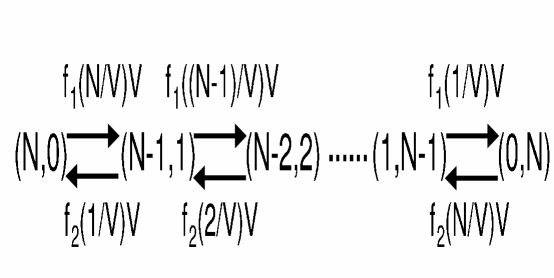
Figure 2:

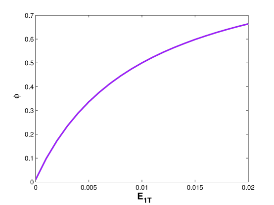
Figure 3:

Figure 4:

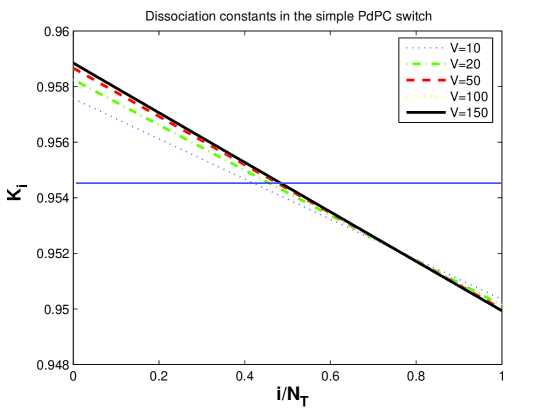
Figure 5:

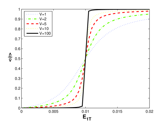
Figure 6:

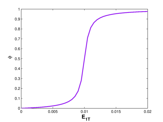
Figure 7:

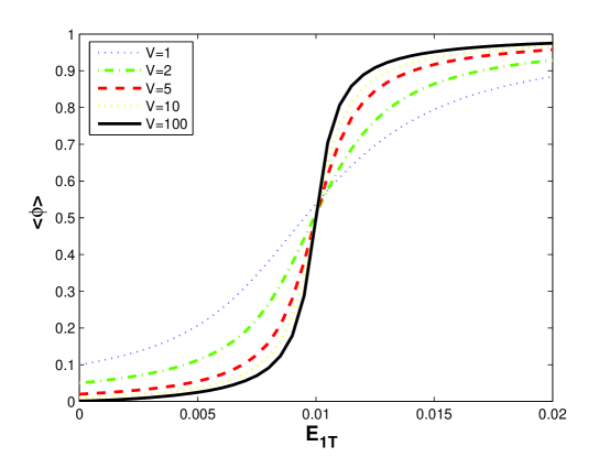
Figure 8:

Figure 9:

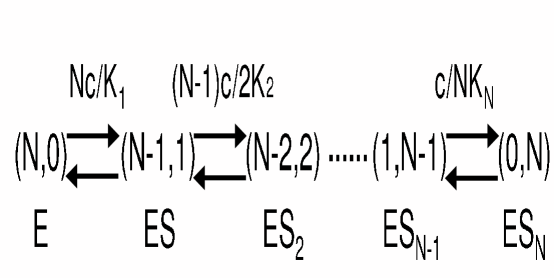
Figure 10:

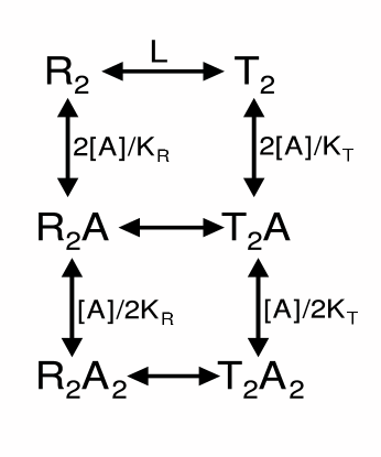
Figure 11:

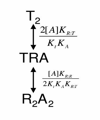
Figure 12:

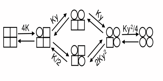
Figure 13:

	Standard Models		Dissociation constants
Temporal	General model(Fig. 2)		$K_{i}=\frac{(N+1-i)f_{2}(i/V)}{if_{1}((N+1-i)/V)}$
cooperativity	Simple PdPC switch model		$K_{i}\approx\frac{\frac{V_{2}^{*}}{K_{2}^{*}}+\frac{V_{1}^{*}}{K_{1}^{*}}}{\frac{V_{2}}{K_{2}}+\frac{V_{1}}{K_{1}}}$
	Ultrasensitive PdPC switch model		$K_{i}\approx\frac{N+1-i}{i}\frac{V_{1}^{*}+V_{2}^{*}}{V_{1}+V_{2}}$
Allosteric	Symmetric	Two sites	$K_{1}=\frac{1+L}{\frac{1}{K_{R}}+\frac{L}{K_{T}}},~{}K_{2}=\frac{\frac{1}{K_{R}}+\frac{L}{K_{T}}}{\frac{1}{K_{R}^{2}}+\frac{L}{K_{T}^{2}}}$
cooperativity	model	$N$ sites	$K_{i}=\frac{\frac{1}{K_{R}^{i-1}}+\frac{L}{K_{T}^{i-1}}}{\frac{1}{K_{R}^{i}}+\frac{L}{K_{T}^{i}}}$
	Sequential	Dimer	$K_{1}=\bar{K}/c,~{}K_{2}=c\bar{K}$
	model	Quaternary	$K_{i}=\frac{1}{K},~{}\frac{3}{(2y+1)K},~{}\frac{2y+1}{3y^{2}K},~{}\frac{1}{Ky^{2}}$

Table 1: Summary: a compare of temporal and allosteric cooperativity models through dissociation constants.

References

• [1] E.H. Fischer, L.M.G. Heilmeyer, and R.H. Haschke, Curr. Top. Cell. Regul. 4, 211 (1971)
• [2] E.G. Krebs, Curr. Top. Cell. Regul. 18, 401 (1980)
• [3] A.V. Hill, Journal of Physiology 40, iv (1910)
• [4] J. Monod, J. Wyman, and J.P. Changeux, J. Mol. Biol. 12, 88 (1965)
• [5] D.E. Koshland Jr., G. Nemethy, and D. Filmer, Biochmistry 5, 365(1966)
• [6] A. Goldbeter, and D.E. Koshland Jr., Proc. Natl. Acad. Sci. USA 78, 6840 (1981)
• [7] D.E. Koshland Jr., A. Goldbeter, and J.B. Stock, Science 217, 220 (1982)
• [8] C.F. Huang, and J.E. Ferrell Jr., Proc. Natl. Acad. Sci. USA 93, 10078 (1996)
• [9] H. Qian, Biophys. Chem. 105, 585 (2003)
• [10] H. Qian, Annu. Rev. Phys. Chem. 58, 113 (2007)
• [11] G. Nicolis, and I. Prigogine, Self-organization in nonequilibrium systems: from dissipative structures to order through fluctuations. (New York: Wiley 1977)
• [12] E.R. Stadtman, and P.B. Chock, Proc. Natl. Acad. Sci. USA 74, 2761 (1977)
• [13] R. Heinrich, B.G. Neel, and T.A. Rapoport: Mol. Cell 9, 957 (2002)
• [14] J.D. Murray, Mathematical biology, 3rd Ed. (New York: Springer 2002)
• [15] C.P. Fall, E.S. Marland, J.M. Wagner, and J.J. Tyson, Computational cell biology. (New York: Springer-Verlag 2002)
• [16] D.T. Gillespie, J. Comp. Phys. 22, 403 (1976)
• [17] D.A. McQuarrie, J. Chem. Phys. 38, 437 (1963)
• [18] C.J. Jachimowski, D.A. McQuarrie, and M.E. Russell, Biochemistry 3, 1732 (1964)
• [19] D.A. McQuarrie, J. Appl. Prob. 4, 413 (1967)
• [20] H. Grabert, P. Hanggi, and I. Oppenheim, Physica l17A, 300 (1983)
• [21] N.G. Van Kampen, Stochastic Processes in Physics and Chemistry. (Amsterdam: North-Holland 1981)
• [22] H. Qian, S. Saffarian and E.L. Elson, Proc. Natl. Acad. Sci. USA 99, 10376 (2002)
• [23] T.S. Zhou, L.N. Chen, and R.Q. Wang, Physica D 211, 107 (2005)
• [24] P.S. Swain, M.B. Elowitz, and E.D. Siggia, Proc. Natl. Acad. Sci. USA 99, 12795 (2002)
• [25] J.S. van Zon, M.J. Morelli, S. Tanase-Nicola, and P.R. ten Wolde, Biophys. J. 91, 4350 2006
• [26] H. Qian, J. Phys. Cond. Matt. 17, S3783 (2005)
• [27] H. Qian, J. Phys. Chem. B. 110, 15063 (2006)
• [28] H. Ge, H. Qian, and M. Qian, Math. Biosci. 211, 132 (2007)
• [29] H. Ge, J. Phys. Chem. B 112, 61 (2007)
• [30] D.A. Beard, and H. Qian, Chemical Biophysics: Quantitative Analysis of Cellular Systems. Cambridge Texts in Biomedical Engineering (Cambridge University Press 2008)
• [31] J. Howard, Mechanics of motor proteins and the cytoskeleton. (Sunderland, MA: Sinauer 2001)
• [32] A. Cornish-Bowden, Fundamentals of enzyme kinetics. 3nd ed. (London: Portland Press 2004)
• [33] J. Elf, J. Paulsson, O.G. Berg, and M. Ehrenberg, Biophys. J. 84, 154 (2003)
• [34] T.G. Kurtz, J. Chem. Phys. 57, 2976 (1972)
• [35] O.G. Berg, J. Paulsson, and M. Ehrenberg, Biophys. J. 79, 1228 (2000)
• [36] J. Monod, J.P. Changeux, and F. Jacob, J. Mol. Biol. 6, 306 (1963)
• [37] G.S. Adair, J. Biol. Chem. 63, 529 (1925)
• [38] H. Qian, and J.A. Cooper, Biophys. J. 47, 2211 (2008)
• [39] J. Ricard, and A. Cornish-Bowden, Eur. J. Biochem. 166, 255 (1987)
• [40] D.E. Koshland Jr., Proc. Natl. Acad. Sci. USA 44, 98 (1958)
• [41] D.E. Koshland Jr., “Mechanisms of transfer enzymes.” 305-306 in The Enzymes. 2nd ed.(Edited by Boyer, P.D., Lardy, H. and Myrback, K.) volume 1, Academic Press, New York 1959
• [42] D.E. Koshland Jr., J. Cell. Comp. Physiol. 54, supplement 1, 245 (1959)
• [43] L. Pauling, Proc. Natl. Acad. Sci. 21, 186 (1935)
• [44] D.E. Koshland Jr., Science 280, 852 (1998)
• [45] L.H. Hartwell, J.J. Hopfield, S. Leibler, and A.W. Murray, Nature(London) 402, C47 (1999)
• [46] E.H. Fischer, and E.G. Krebs, J. Mol. Chem. 216, 121 (1955)
• [47] D.J. Wilkinson, Stochastic Modelling for Systems Biology. (Chapman and Hall/CRC 2006) p. 147
• [48] D.Q. Jiang, M. Qian, and M.P. Qian, Mathematical theory of nonequilibrium steady states - On the frontier of probability and dynamical systems. Lect. Notes Math. 1833 (Berlin: Springer-Verlag 2004) Chap.2
• [49] J. Schnakenberg, Rev. Modern Phys. 48, 571 (1976)
Refer to caption