Edwards curves and CM curves

Abstract

Edwards curves are a particular form of elliptic curves that admit a fast, unified and complete addition law. Relations between Edwards curves and Montgomery curves have already been described. Our work takes the view of parameterizing elliptic curves given by their $j$-invariant, a problematic that arises from using curves with complex multiplication, for instance. We add to the catalogue the links with Kubert parameterizations of $X_{0}(2)$ and $X_{0}(4)$. We classify CM curves that admit an Edwards or Montgomery form over a finite field, and justify the use of isogenous curves when needed.

1 Introduction

An Edwards curve [10] is a particular form of an elliptic curve that leads to fast, unified and complete addition formulas [5, 3]. Using inverted Edwards coordinates yields the fastest formulas for adding points on such a curve [6]. One may consult [4] for comparisons of multiplication on a curve, as well as for many references.

Following [7], the equation of a twisted Edwards curve is

$$ax^{2}+y^{2}=1+dx^{2}y^{2}$$ (1)

where $a$, $d$ non zero elements of a field $\mathbb{K}$. An Edwards curve corresponds to $a=1$.

The completeness of the addition equations occurs only when $a$ is a square and $d$ is not a square in the base field, in which case there are no rational singular points on the curve. We will say that an elliptic curve $E$ can be put in twisted Edwards form if there is a (rational) change of variables leading to an equation of the type (1). We will use the term complete Edwards form when $a$ is a square (including the case $a=1$ of course) and $d$ is not a square.

Recognizing an Edwards curve is relatively easy [7, Theorem 3.3].

Theorem 1

If $\mathbb{K}$ is of characteristic different from $2$, the curve $E$ is birationally equivalent to an Edwards curve if and only if $E(\mathbb{K})$ has a point of order 4.

By [5, Theorem 2.1], if $\mathbb{K}$ is finite, the curve is complete if $E(\mathbb{K})$ has a point of order 4 and a unique point of order 2.

Another form of elliptic curve is the Montgomery form

$$E:By^{2}=x^{3}+Ax^{2}+x$$ (2)

with $A\neq\pm 2$, $B\neq 0$ (see [15]). Theorem 3.2 of [7] is

Theorem 2

If $\mathbb{K}$ has characteristic different from 2, then every curve in Montgomery form is birationally equivalent to a twisted Edwards curve, the converse being true.

In many applications (factoring, elliptic curve cryptography), one has the choice of the curve and parameterization. In other contexts, such as primality proving or the CM method, a curve is given via its $j$-invariant and it may seem interesting to find an appropriate parameterization starting from $j$.

Since elliptic curves having a rational $2$-torsion or $4$-torsion point can be parameterized using modular curves, we will indicate how to relate this to Edwards or Montgomery forms via Kubert’s equations. This will be the task of Section 2, together with more general properties of the $2$-torsion and $4$-torsion. Section 3 is interested in CM properties of elliptic curves, and use classical results to investigate when the discriminant of a curve having CM by a quadratic order is a square in the corresponding ring class field. Results of Section 2 and 3 are then applied in Section 4 on curves over finite fields. Moreover, we show how to replace a curve that does not admit a complete Edwards form by an isogenous curve having such a form, thus extending [7, Section 5].

2 Properties of the $2$-torsion

2.1 Generalities

We collect here some properties of the $2$-torsion group of an elliptic curve whose equation will be taken as $Y^{2}=F(X)=X^{3}+a_{2}X^{2}+a_{4}X+a_{6}$, with coefficients in some field $\mathbb{K}$ of characteristic $\neq 2$ (see [20]). We will note $e_{1}$, $e_{2}$, $e_{3}$ for the roots of $F(X)$ (over some subfield of an algebraic closure of the base field $\mathbb{K}$). Remember that the discriminant of the curve is

$$\Delta(E)=-64\,a_{6}\,{a_{2}}^{3}+16\,{a_{4}}^{2}{a_{2}}^{2}+288\,a_{4}\,a_{6}\,a_{2}-64\,{a_{4}}^{3}-432\,{a_{6}}^{2}.$$

Two curves $E:Y^{2}=X^{3}+a_{2}X^{2}+a_{4}X+a_{6}$ and $E^{\prime}:Y^{2}=X^{3}+a_{2}^{\prime}X^{2}+a_{4}^{\prime}X+a_{6}^{\prime}$ are isomorphic if and only if there exists $(u,r)$ in $\mathbb{K}^{2}$ with $u\neq 0$ such that the following system has a solution:

$$\left\{\begin{array}[]{lcl}u^{2}a_{2}^{\prime}&=&a_{2}+3r,\\ u^{4}a_{4}^{\prime}&=&a_{4}+2ra_{2}+3r^{2},\\ u^{6}a_{6}^{\prime}&=&a_{6}+ra_{4}+r^{2}a_{2}+r^{3},\\ \end{array}\right.$$ (3)

the isomorphism sending $E$ to $E^{\prime}$ via

$$(x,y)\mapsto(u^{2}x+r,u^{3}y).$$

The $n$-th division polynomial will be denoted $f_{n}(X)$ and we will be interested mostly in the properties of

$$f_{4}(X)={X}^{6}+2\,a_{2}\,{X}^{5}+5\,a_{4}\,{X}^{4}+20\,a_{6}\,{X}^{3}+\left(20\,a_{2}\,a_{6}-5\,{a_{4}}^{2}\right){X}^{2}$$

$$\hskip 85.35826pt+\left(-4\,a_{4}\,a_{6}+8\,{a_{2}}^{2}a_{6}-2\,a_{2}\,{a_{4}}^{2}\right)X+4\,a_{4}\,a_{6}\,a_{2}-{a_{4}}^{3}-8\,{a_{6}}^{2}.$$

Note that the discriminant of $F(X)$ is $\Delta(E)/16$ and that of $f_{4}(X)$ is $-\Delta(E)^{5}/4$.

2.2 Curves with at least one torsion point

We now turn our attention towards the $2$-torsion and $4$-torsion of $E$. If $E$ has a rational $2$-torsion point, then $F(X)$ will have one or three roots over $\mathbb{K}$. We will call these cases type I or type III curves.

Let us begin with some general results on the curve $E$ of equation $Y^{2}=F(X)=(X-x_{0})(X^{2}+CX+D)$. Elementary computations show the following list of results:

$$\Delta(E)=16\left(x_{0}^{2}+Cx_{0}+D\right)^{2}\left({C}^{2}-4\,D\right),$$

which cannot be zero since $E$ is an elliptic curve. Furthermore

$$f_{4}(X)=\mathcal{P}_{2}(X)\mathcal{P}_{4}(X)$$ (4)

where $\mathcal{P}_{i}$ has degree $i$ and

$$\mathcal{P}_{2}(X)={X}^{2}-2\,x_{0}\,X-Cx_{0}-D,$$

$$\mathcal{P}_{4}(X)={X}^{4}+2\,C\,{X}^{3}+6\,D\,{X}^{2}+\left(-8\,x_{0}\,D+2\,CD+2\,x_{0}\,{C}^{2}\right)X+(4D-{C}^{2})x_{0}^{2}+{D}^{2}.$$

The discriminants are

$$\mathrm{Disc}(\mathcal{P}_{2})=4(x_{0}^{2}+Cx_{0}+D)=4\mathcal{D}_{2},$$

$$\mathrm{Disc}(\mathcal{P}_{4})=-2^{8}\,\left({C}^{2}-4\,D\right)^{3}\left(x_{0}^{2}+Cx_{0}+D\right)^{3}=-2^{8}\left({C}^{2}-4\,D\right)^{3}\mathcal{D}_{2}^{3}.$$

Lemma 3

The polynomials $\mathcal{P}_{2}$ and $\mathcal{P}_{4}$ do not have a common root.

Proof: We compute

$$\mathrm{Resultant}_{X}(\mathcal{P}_{2}(X),\mathcal{P}_{4}(X))=-16(x_{0}^{2}+Cx_{0}+D)^{3}(C^{2}-4D),$$

and both terms are non-zero, otherwise $F$ would have multiple roots. $\Box$

2.2.1 Curves of type I

Such a curve has equation $Y^{2}=F(X)=(X-x_{0})(X^{2}+CX+D)$ with the quadratic polynomial irreducible. Let us study division by $2$ on $E$. Let $P=(x,y)$ be a rational $4$-torsion point. Then $[2]P$ is the $2$-torsion point $(x_{0},0)$. Writing the formulas for multiplication by $2$, we get

$$\frac{F^{\prime}(x)^{2}}{4F(x)}-(C-x_{0})-2x=x_{0}$$

or $x$ is a root of

$$\mathcal{P}_{x_{0}}(X)=\left({X}^{2}-2\,x_{0}\,X-D-x_{0}\,C\right)^{2}=\mathcal{P}_{2}(X)^{2}.$$

Corollary 4

If $E$ is of type I, the polynomial $\mathcal{P}_{4}$ cannot have a rational root.

Proof: Assume on the contrary that $\mathcal{P}_{4}$ has a rational root $z$. Then $z$ would be sent by multiplication by 2 on the unique rational $2$-torsion abscissa $x_{0}$. This would imply $\mathcal{P}_{x_{0}}(z)=0$, which by Lemma 3 is impossible. $\Box$

Proposition 5

The curve $E:Y^{2}=(X-x_{0})(X^{2}+CX+D)$ of type I has two rational $4$-torsion points if and only if $\mathcal{D}_{2}$ is a square.

Proof: The rational roots of the polynomial $f_{4}$ are that of $\mathcal{P}_{2}$ by Corollary 4. Writing $z^{2}=x_{0}^{2}+Cx_{0}+D$, the polynomial $\mathcal{P}_{2}$ has roots $x_{\pm}=x_{0}\pm z$. Letting $y_{\pm}$ denote the ordinates, we find that $y_{\pm}^{2}=z^{2}(C+2(x_{0}\pm z))$. Since

$$(C+2(x_{0}+z))(C+2(x_{0}-z))=C^{2}-4D$$

we see that exactly one of the factors is a square, leading to two rational $4$-torsion points. $\Box$

2.2.2 Curves of type III

Suppose now $E:Y^{2}=F(X)=(X-e_{1})(X-e_{2})(X-e_{3})$ is of type III with all $e_{i}\in\mathbb{K}$. Then

$$\Delta(E)=2^{4}(e_{1}-e_{2})^{2}(e_{1}-e_{3})^{2}(e_{2}-e_{3})^{2},$$

and the polynomial $\mathcal{P}_{4}$ will factor into three quadratics

$$f_{4}(X)=\left({X}^{2}-2\,e_{1}\,X+e_{1}(e_{2}+e_{3})-e_{2}\,e_{3}\right)$$

$$\hskip 56.9055pt\times\left({X}^{2}-2\,e_{2}\,X+e_{2}(e_{1}+e_{3})-e_{1}\,e_{3}\right)$$

$$\hskip 56.9055pt\times\left({X}^{2}-2\,e_{3}\,X+e_{3}(e_{1}+e_{2})-e_{1}\,e_{2}\right)$$

of respective discriminants $4(e_{1}-e_{3})(e_{1}-e_{2})$, $4(e_{2}-e_{1})(e_{2}-e_{3})$, $4(e_{3}-e_{1})(e_{3}-e_{2})$. If $\Delta(E)$ is a square in $\mathbb{K}$, then one or all these discriminants are squares, so that the corresponding factors split. Suppose $4(e_{1}-e_{3})(e_{1}-e_{2})=\delta_{1}^{2}$. Then the two roots of

$$\mathcal{Q}_{e_{1}}(X)={X}^{2}-2\,e_{1}\,X+e_{1}(e_{2}+e_{3})-e_{2}\,e_{3}$$

are $x_{\pm}=2e_{1}\pm\delta_{1}$. The corresponding ordinates satisfy

$$y_{\pm}^{2}=\delta_{1}^{2}/4(2x_{\pm}-e_{2}-e_{3}).$$

2.3 Properties of $2$-isogenies

The following formulas come from the use of Vélu’s formulas (already given in [9]):

Proposition 6

Assume that $E:Y^{2}=X^{3}+a_{2}X^{2}+a_{4}X+a_{6}$ has a rational point of order $2$, noted $P=(x_{0},0)$. Put $t=3x_{0}^{2}+2a_{2}x_{0}+a_{4}$ and $w=x_{0}t$. Then an equation of $E/\langle P\rangle$ is $E_{1}:Y_{1}^{2}=X_{1}^{3}+A_{2}X_{1}^{2}+A_{4}X_{1}+A_{6}$ where $A_{2}=a_{2}$, $A_{4}=a_{4}-5t$, $A_{6}=a_{6}-4a_{2}t-7w$. Moreover, the isogeny $I_{1}:E\rightarrow E_{1}$ sends $(X,Y)$ to

$$(X_{1},Y_{1})=\left(X+\frac{t}{X-x_{0}},Y\left(1-\frac{t}{(X-x_{0})^{2}}\right)\right).$$

The typical use of the Proposition 5 is given now. It will prove essential in the isogeny volcano approach later on.

Corollary 7

Let $E$ be a type III curve. If $E_{1}=E/\langle(e_{1},0)\rangle$ is a type I curve, then $E_{1}$ admits a complete Edwards form.

Proof: An equation for $E_{1}=E/\langle(e_{1},0)\rangle$ is

$$E_{1}:Y^{2}=(X-x_{0})(X^{2}+CX+D)$$

with

$$x_{0}=e_{2}+e_{3}-e_{1},\quad C^{2}-4D=16(e_{1}-e_{2})(e_{1}-e_{3}),\quad x_{0}^{2}+Cx_{0}+D=(e_{2}-e_{3})^{2}.$$

If $e_{2}$ and $e_{3}$ are rational, then $\mathcal{D}_{2}$ is a square and we are done. $\Box$

2.4 Montgomery parameterizations

A Montgomery form of an elliptic curve is some equation $By^{2}=x^{3}+Ax^{2}+x$ with $A\neq\pm 2$ and $B\neq 0$. This shows that only curves having a rational $2$-torsion point can be of this form. Curves having a $2$-torsion points are points on the modular curve $X_{0}(2)$, an equation of which is

$$j=\frac{(u+16)^{3}}{u}.$$ (5)

Note also that

$$j-1728=\frac{(u+64)(u-8)^{2}}{u}$$

An equation for an elliptic curve $E$ of given invariant $j$ is

$$Y^{2}=X^{3}+\frac{3j}{1728-j}c^{2}X+\frac{2j}{1728-j}c^{3}$$ (6)

(with $c$ present to accommodate twists). We compute

$$\Delta(E)=2^{12}3^{6}c^{6}\frac{j^{2}}{(j-1728)^{3}}=2^{12}3^{6}c^{6}\,{\frac{\left(u+16\right)^{6}u}{\left(u+64\right)^{3}\left(u-8\right)^{6}}}.$$

Plugging equation (5) in (6), we find that the cubic has rational root $-c(u+16)/(u-8)$. The quadratic factor has discriminant $\mathcal{D}_{1}=9c^{2}u(u+64)(u+16)^{2}$. Moreover

$$\mathcal{D}_{2}=2^{6}\times 3^{2}c^{2}(u+16)^{2}(u-8)^{2}(u+64).$$ (7)

Let us show how we can recover a Montgomery parameterization for these curves. Setting $X=X^{\prime}-c\frac{u+16}{u-8}$, this transforms (6) into

$$Y^{2}={X^{\prime}}^{3}-3\,c\,{\frac{\left(u+16\right){{X^{\prime}}}^{2}}{u-8}}+144\,c^{2}\,{\frac{\left(u+16\right)^{2}{X^{\prime}}}{\left(u+64\right)\left(u-8\right)^{2}}}.$$

If $u+64=v^{2}$, then setting $X^{\prime}=kX^{\prime\prime}$ with

$$k=12\,c\,{\frac{u+16}{\left(u-8\right)v}}$$

leads to the Montgomery form

$$\frac{1}{k}(Y/k)^{2}={X^{\prime\prime}}^{3}-\frac{v}{4}{X^{\prime\prime}}^{2}+{X^{\prime\prime}}.$$

In Section 3, we will express $u$ as one of Weber’s functions and investigate when $u+64$ is a square in some ring class field.

2.5 Kubert parameterizations

In [14] are given all parameterizations of curves over $\mathbb{Q}$ having prescribed torsion structure. Of particular relevance to Edwards curves is the parameterization for curves $E$ containing the torsion group $\mathbb{Z}/4\mathbb{Z}$. Letting $b\in\mathbb{Q}$ such that $b^{4}(1+16b)\neq 0$, we get the parameterization

$$\mathcal{EK}_{b}:Y^{2}=(X-4b)\left({X}^{2}+X-4b\right).$$

The curve $\mathcal{EK}_{b}$ has a unique point of order $2$, $(4b,0,1)$. The division polynomial $f_{4}$ factors as

$$f_{4}(X)=X\left(X-8\,b\right)\left({X}^{4}+2\,{X}^{3}-24\,b{X}^{2}+128\,{b}^{2}X-256\,{b}^{3}\right).$$

The two rational roots are: $0$, which leads to two rational points $(0,\pm 4b,1)$ and $8b$, for which $Y^{2}=16b^{2}(16b+1)$. Note that the $j$-invariant of $\mathcal{EK}_{b}$ is:

$$j={\frac{\left(16\,{b}^{2}+16\,b+1\right)^{3}}{{b}^{4}\left(16\,b+1\right)}}.$$

Writing $w=1/b$ leads to

$$j={\frac{\left({w}^{2}+16\,w+16\right)^{3}}{w\left(16+w\right)}}$$

and we see that setting $u=w^{2}+16w$ makes $j$ of the form (5) and that $u+64=(w+8)^{2}$, so that we get a Montgomery form in that case too. With the notations of the preceding Section:

$$\mathcal{D}_{1}=9c^{2}w^{2}(w+8)^{2}(w^{2}+16w+16)^{2}(1+16/w),$$

$$\mathcal{D}_{2}=2^{6}\times 3^{2}c^{2}(w^{2}+16w+16)^{2}(w^{2}+16w-8)^{2}(w+8)^{2}.$$

This shows the following

Proposition 8

For any $w\neq 0$, the curve $E$ associated to $w$ admits a Montgomery form. Moreover, if $1+16/w$ is not a square, $E$ admits a complete Edwards form.

Making $w=16d/(a-d)$ or $a=d(1+16/w)$ yields directly

$$J=\frac{16(a^{2}+14ad+d^{2})^{3}}{ad(a-d)^{4}}$$

and this is precisely the invariant of a twisted Edwards curve.

The proof of the following is rather tedious and is preferably done using a computer (and Maple in our case).

Proposition 9

Suppose $E$ is of type I: $F(X)=(X-x_{0})(X^{2}+CX+D)$ with the quadratic polynomial irreducible and $x_{0}^{2}+Cx_{0}+D=z^{2}$. Then $E$ is isomorphic to $\mathcal{EK}_{b}$ with

$$r=\frac{(1-4b)\,{u}^{2}+x_{0}-C}{3},$$

$$u^{2}=C+2(x_{0}\pm z),$$

whichever sign yields a square (cf. Proposition 5) and

$$b=\mp 1/4\,{\frac{z}{C+2\,(x_{0}\pm\,z)}}\text{ or }b=-1/4\,{\frac{\pm 7\,z+8\,x_{0}+4\,C}{C+2\,(x_{0}\pm\,z)}}.$$

Proposition 10

The Kubert curve $\mathcal{EK}_{b}$ is birationally equivalent to the Edwards curve of parameter $d=16b+1$. If $16b+1$ is not a square, then the curve is complete.

Proof: If we plug these values in the transformation formulae of [5, Theorem 2.1], we get

$$a_{2}=2b+1/4,a_{4}=b^{2},d=16b+1,r_{1}/(1-d)=1/16$$

so that the curve $\mathcal{EK}_{b}$ is birationally equivalent to

$$E^{\prime}:(s/4)^{2}=r^{3}+a_{2}r^{2}+a_{4}r,$$

which is shown in the same theorem to be birationally equivalent to $x^{2}+y^{2}=1+dx^{2}y^{2}$. $\Box$

3 CM curves

In the CM method, we use elliptic curves that are constructed given their invariant. We have the choice of the explicit form of the equation to be used and it is natural to ask when a CM curve can be written in Edwards or Montgomery form (see [2] for a possible use in primality proving [1]).

3.1 Theorems over $\mathbb{C}$

Let $\mathcal{E}$ have complex multiplication by an order $\mathcal{O}$ of discriminant $D=f^{2}D_{K}$ in an imaginary quadratic field $\mathbf{K}=\mathbb{Q}(\sqrt{D_{K}})$ of discriminant $D_{K}$. Such a curve can be built using its $j$-invariant that is a root of the so-called class polynomial $H_{D}(X)$, that generates the ring class field $\mathbf{K}_{\mathcal{O}}=\mathbf{K}(j(\mathcal{O}))$. The roots of $H_{D}(X)$ are of the form $j(\alpha)$ where $\alpha$ is the root of positive imaginary part of $AX^{2}+BX+C$ with $(A,B,C)$ a reduced primitive quadratic form of discriminant $B^{2}-4AC=D=\mathrm{Disc}(\alpha)$.

Given $j(\alpha)$ (in other words, any root of $H_{D}(X)$), we can use equation (6) for $\mathcal{E}(\alpha)$ and look for cases where $\Delta(\mathcal{E}(\alpha))$ is a square in $\mathbf{K}_{\mathcal{O}}$. These results will translate in equivalent properties over finite fields. It is natural for this to introduce the Weber function $\gamma_{3}$ satisfying $\gamma_{3}(\alpha)^{2}=j(\alpha)-1728$. We rephrase [18, Satz (5.2)] (see also [19]) as:

Theorem 11

(a) When $D$ is odd, $\Delta(\mathcal{E}(\alpha))$ is a square in $\mathbb{Q}(\alpha,j(\alpha))$.

(b) When $D$ is even, $\Delta(\mathcal{E}(\alpha))$ is a square in $\mathbb{Q}(j(2\alpha))$.

Proof: (a) When $D$ is odd $\sqrt{D}\gamma_{3}(\alpha)$ is a class invariant and we write

$$j(\alpha)-1728=\left(\frac{\sqrt{D}\gamma_{3}(\alpha)}{\sqrt{D}}\right)^{2}.$$

(b) We use $\mathbb{Q}(\gamma_{3}(\alpha))=\mathbb{Q}(j(2\alpha))$. $\Box$

To understand when CM curves have rational $2$-torsion points, we use some other Weber functions, namely $\mathfrak{f}(\alpha)$, $\mathfrak{f}_{1}(\alpha)$ and $\mathfrak{f}_{2}(\alpha)$ that satisfy

$$j(\alpha)=\frac{(-\mathfrak{f}(\alpha)^{24}+16)^{3}}{-\mathfrak{f}(\alpha)^{24}}=\frac{(\mathfrak{f}_{1}(\alpha)^{24}+16)^{3}}{\mathfrak{f}_{1}(\alpha)^{24}}=\frac{(\mathfrak{f}_{2}(\alpha)^{24}+16)^{3}}{\mathfrak{f}_{2}(\alpha)^{24}},$$

in other words, $-\mathfrak{f}(\alpha)^{24}$, $\mathfrak{f}_{1}(\alpha)^{24}$ and $\mathfrak{f}_{2}(\alpha)^{24}$ are the roots of (5). The numbers $\mathfrak{f}(\alpha)^{24}$, $\mathfrak{f}_{1}(\alpha)^{24}$ or $\mathfrak{f}_{2}(\alpha)^{24}$ are very often class invariants, that is elements of $\mathbb{Q}(j(\alpha))$; sometimes they are in $\mathbb{Q}(\alpha,j(\alpha))$. Moreover small powers of these functions are very often elements of $\mathbb{Q}(j(r\alpha))$ for some $r=2^{\pm n}$, as can be seen from [18] for instance.

To go further, we introduce the generalized Weber function

$$\mathfrak{w}_{N}(z)^{s}=(\eta(z/N)/\eta(z))^{s}$$

where $\eta$ is Dedekind’s function and $N$ an integer and $s$ some integer related to $N$. These functions are modular for $\Gamma^{0}(N)$ and give a model for $X^{0}(N)$ (equivalently $X_{0}(N)$). In particular [11]

Theorem 12

Let $\alpha=\frac{-B+\sqrt{D}}{2A}$ be a root associated to the primitive reduced quadratic form $[A,B,C]$ of discriminant $D=B^{2}-4AC$. If $B^{2}\equiv D\bmod 16$ has a solution in $B$ (equivalently $D\bmod 16\in\{0,1,4,9\}$), then $\mathbb{Q}(j(\alpha))\subset\mathbb{Q}(\mathfrak{w}_{4}^{8}(\alpha))\subset\mathbb{Q}(\alpha,j(\alpha))$.

From this

Corollary 13

Let $D\bmod 16\in\{0,1,4,9\}$. Then $\mathcal{E}(j(\alpha))$ admits a Montgomery form.

Proof: Use the fact that the modular equation linking $j(z)$ and $\mathfrak{w}_{4}(z)$ is precisely

$$J={\frac{\left({w}^{2}+16\,w+16\right)^{3}}{w\left(16+w\right)}}$$

which sends us back to Section 2.5. $\Box$

4 Properties of the $2$-torsion over prime finite fields

4.1 Splitting properties

Part of what follows can also be found in [21]. Let $\mathbb{K}$ be a prime finite field of characteristic $p>2$. The following result is classical and taken from [22]. It will help us study the splitting properties of $F(X)$ and $f_{4}(X)$ over a finite field. Note that $F(X)$ and $f_{4}(X)$ have no square factor (since $\Delta(E)\neq 0$ for $E$ to be an elliptic curve).

Theorem 14

Let $f(X)$ be a squarefree polynomial of degree $d$ and $n$ its number of irreducible factors modulo $p$. Then

$$\genfrac{(}{)}{1.0pt}{}{\mathrm{Disc}(f)}{p}=(-1)^{d-n}.$$

This gives us immediately.

Proposition 15

Let $p$ be an odd prime. The curve $E$ has exactly one $2$-torsion point over $\mathbb{F}_{p}$ if and only if $\genfrac{(}{)}{1.0pt}{}{\Delta(E)}{p}=-1$. In that case, and writing $n_{4}$ for the number of irreducible factors of $f_{4}$, one has

$$(-1)^{n_{4}}=-\genfrac{(}{)}{1.0pt}{}{-\mathcal{D}_{2}}{p}.$$

Proof: We have

$$\genfrac{(}{)}{1.0pt}{}{\mathrm{Disc}(\mathcal{P}_{4})}{p}=\genfrac{(}{)}{1.0pt}{}{-1}{p}\genfrac{(}{)}{1.0pt}{}{{C}^{2}-4\,D}{p}\genfrac{(}{)}{1.0pt}{}{\mathcal{D}_{2}}{p}.$$

If $E$ has a unique $2$-torsion point, then

$$\genfrac{(}{)}{1.0pt}{}{{C}^{2}-4\,D}{p}=-1$$

which yields the result. $\Box$

When a polynomial $P(X)$ has factors of degrees $d_{1}$, $\ldots$, $d_{k}$ over $\mathbb{K}$, we will denote this splitting as $(d_{1})\cdots(d_{k})$. The following Proposition describes the splittings of $\mathcal{P}_{2}$ and $\mathcal{P}_{4}$.

Proposition 16

Let $E:Y^{2}=F(X)=(X-x_{0})(X^{2}+CX+D)$ be of type I. The splittings of $\mathcal{P}_{2}$ and $\mathcal{P}_{4}$ can be found in the following table:

$$\begin{array}[]{|c||c|c||c|c|}\hline\cr&\lx@intercol\hfil\genfrac{(}{)}{1.0pt}{}{\mathcal{D}_{2}}{p}=+1\hfil\lx@intercol\vrule\lx@intercol\vrule\lx@intercol&\lx@intercol\hfil\genfrac{(}{)}{1.0pt}{}{\mathcal{D}_{2}}{p}=-1\hfil\lx@intercol\vrule\lx@intercol\\ \hline\cr&\mathcal{P}_{2}&\mathcal{P}_{4}&\mathcal{P}_{2}&\mathcal{P}_{4}\\ \hline\cr p\equiv 1\bmod 4&(1)(1)&(4)&(2)&(2)(2)\\ p\equiv 3\bmod 4&(1)(1)&(2)(2)&(2)&(4)\\ \hline\cr\end{array}$$

Proof: Assume first that $\genfrac{(}{)}{1.0pt}{}{\mathcal{D}_{2}}{p}=+1$. If $p\equiv 1\bmod 4$, $\mathcal{P}_{4}$ should have an odd number of irreducible factors, leading to $(4)$ or $(1)(1)(2)$ but Corollary 4 rules out $(1)(1)(2)$. If $p\equiv 3\bmod 4$, then $\mathcal{P}_{4}$ should have an even number of factors or be of type $(1)(3)$ and $(2)(2)$ and only the latter one is possible.

The proof for the case $\genfrac{(}{)}{1.0pt}{}{\mathcal{D}_{2}}{p}=-1$ is symmetrical and we omit it. $\Box$

4.2 Reduction of CM curves over a finite field

If $p$ splits in the ring class field $\mathbf{K}_{\mathcal{O}}=\mathbf{K}(j(\mathcal{O}))$, i.e., $p=(U^{2}-DV^{2})/4$, then we can reduce $\mathcal{E}$ modulo a prime factor of $p$ in $\mathbf{K}_{\mathcal{O}}$ to get a curve $E/\mathbb{F}_{p}$ of cardinality $p+1-U$. This is the heart of the CM-method, which is a building block in ECPP for instance [1, 17].

Conversely, a (non supersingular) elliptic curve $E/\mathbb{F}_{p}$ has complex multiplication by an order $\mathcal{O}$ in an imaginary quadratic field $\mathbf{K}$. In details, if $E$ has cardinality $p+1-U$, write $\mathrm{Disc}(\pi)=U^{2}-4p=V^{2}D_{K}$ for the discriminant of the Frobenius $\pi$ of the curve. We have $\mathbb{Z}[\pi]\subset\mathcal{O}\subset\mathcal{O}_{K}$, where $\mathcal{O}_{K}$ is the ring of integers of $\mathbf{K}$. Noting $f$ for the conductor of the order $\mathcal{O}$, we have $\mathrm{Disc}(\mathcal{O})=f^{2}D_{K}$, with $f\mid V$.

The volcano structure [13] (see also [12]) describes the relationships between inclusions of orders in $\mathcal{O}_{K}$ and the structure of elliptic curves having CM by these orders. Rational $2$-torsion points are in one-to-one correspondence with isogenies of degree $2$ (see Proposition 6 for an illustration of this). The volcano for the prime 2 has the shape of Figure 1 (in case $(2)$ splits in $\mathcal{O}_{K}$). The crater is formed of horizontal isogenies (if any) and each curve on the crater has one isogeny down. Any curve strictly between the crater and the bottom has one isogeny up and two down.

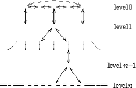
Figure 1: Isogeny volcano for the prime $2$.

General properties of the volcano can be used to meet some of our needs. The following results justifies the idea already presented in [7, Section 5].

Theorem 17

Assume $E/\mathbb{F}_{p}$ is of type III. There exists a curve $E^{\prime}/\mathbb{F}_{p}$ isogenous to $E$ that is of type I. Moreover, $E^{\prime}$ admits a complete Edwards form.

Proof: The proof of Proposition 17 comes directly from [13, Proposition 23]. It is enough to find a curve at the bottom of the volcano for prime $2$. Letting $\mathrm{Disc}(\pi)=U^{2}-4p=D_{K}V^{2}$ and $2^{n}\mid\mid V$, this curve will be at level $n$.

The last part comes from Corollary 7. $\Box$

From a practical point of view, procedure FindDescendingPath of [12] can be used to do just this. Now we apply the results of Section 2. Starting from our curve $E$, we build a path

$$E\rightarrow E_{1}\rightarrow\cdots\rightarrow E_{n-1}\rightarrow E^{\prime}$$

with $E_{n-1}$ of type III and $E^{\prime}$ of type I. Proposition 6 can be used to transport points if needed.

Remarks.

1. We can easily modify procedure FindDescendingPath so that we can keep track of the $2$-torsion points we encounter, so that we obtain a root of $E/\langle(e_{1},0)\rangle$ from the $e_{i}$’s, see Corollary 7.

2. If we know that $E$ has CM by $\mathcal{O}_{K}$, then we can simplify FindDescendingPath by discarding horizontal invariants using the class polynomial, so that we are left with just one descending path.

Numerical examples. Consider $E:Y^{2}=X^{3}+X+2$ over $\mathbb{F}_{1009}$. We find

$$\begin{array}[]{|c|c|c|}\hline\cr i&E_{i}&2\text{-torsion}\\ \hline\cr 0&{[1,2]}&\{463,547,1008\}\\ 1&{[990,30]}=E_{0}/\langle(1008,0)\rangle&\{2,3,1004\}\\ 2&{[950,871]}=E_{1}/\langle(3,0)\rangle&\{265,750,1003\}\\ 3&{[1003,17]}=E_{2}/\langle(750,0)\rangle&\{518\}\\ \hline\cr\end{array}$$

and $E_{3}$ admits $(247,\pm 19)$ has rational $4$-torsion points, and therefore is birationally equivalent to a complete Edwards curve.

We end this section with the following count, that is easily deduced from the volcano structure.

Proposition 18

The set of invariants of complete Edwards curves is formed of the $j$-invariants on the floor of the $2$-volcano. If $4p=t^{2}-v^{2}2^{n}D_{K}$, where $D_{K}$ is fundamental and $v$ odd, there is a total of $2^{n-1}(2-\genfrac{(}{)}{1.0pt}{}{D_{K}}{2})h(D_{K})$ such invariants, where $\genfrac{(}{)}{1.0pt}{}{D_{K}}{2}$ denotes the Kronecker symbol.

4.3 Classifying Montgomery and Edwards curves over finite fields

We assume throughout that $E/\mathbb{F}_{p}$ is the reduction of a curve $\mathcal{E}(\alpha)$ having CM by an order of discriminant $D$ so that in particular $p=(U^{2}-DV^{2})/4$. The aim of this section is to prove the following results.

Theorem 19

If $D$ is fundamental, then $E$ does not admit a complete Edwards form.

Theorem 20

Suppose $E/\mathbb{F}_{p}$ has CM by $\mathcal{O}$ of discriminant $D$. The following Table summarizes the properties of the reduction of $\mathcal{E}(\alpha)$:

$D$	$V$	2-torsion	Montgomery form	Edwards form
$D$ odd
$1\bmod 8$	–	type III	yes	twisted, not complete
$5\bmod 8$	even	type III	yes	twisted, not complete
	odd	none	–	–
$D$ even
$0,4\bmod 16$	even	type III	yes	twisted, not complete
	odd	type I	yes	complete
$8,12\bmod 16$	even	type III	yes/no	twisted at best
	odd	type I	no	no

The following result is taken from [16] (precised by Theorem 11) and starts our proof of Theorem 19.

Proposition 21

The quantity $\Delta(E)$ is a square modulo $p=(U^{2}-DV^{2})/4$ in the following cases:

(a) $D$ odd;

(b) $D$ even and $2\mid V$.

Together with Proposition 15, this proves part of our theorem.

Proof: By Section 2.2.2, any curve of type III admits rational roots for $f_{4}(X)$, but not always rational ordinates.

Suppose $D$ satisfies one of the conditions of Proposition 21. In that case, we see that $E$ has zero or three $2$-torsion points. If we prove that $E$ admits at least one, we get three of them.

If $D\equiv 1\bmod 8$, the ideal $(2)$ splits in $\mathcal{O}_{K}$ and there are three (distinct) rational isogenies starting from $E$, corresponding to three $2$-torsion points ([13, Proposition 23] again). Then apply Corollary 13.

It is clear that when $D\equiv 5\bmod 8$ and $V$ odd, then $E$ has no rational $2$-torsion points at all. With $p=(U^{2}-DV^{2})/4$, we must have $U$ and $V$ of the same parity. Having a $2$-torsion point is equivalent with $U$ even and therefore $V$ even.

Suppose now $D=-4m$ is even. Then $U$ is even, so that $E$ admits at least one $2$-torsion point. If $V$ is even, $\Delta$ is a square, forcing the splitting $(1)(1)(1)$. The cases $m=0,3\bmod 4$ come from Corollary 13.

Dirichlet’s theorem (see [8, Ch. 4]), gives us necessary arithmetical conditions on $p$ to split as $(U^{2}-DV^{2})/4$. For an integer $p$, let $\chi_{4}(p)=\genfrac{(}{)}{1.0pt}{}{-1}{p}$ and $\chi_{8}(p)=\genfrac{(}{)}{1.0pt}{}{2}{p}$. The generic characters of $D$ are defined as follows:

• $\genfrac{(}{)}{1.0pt}{}{p}{q}$ for all odd primes $q$ dividing $D$;

• if $D$ is even:

  • $\chi_{4}(p)$ if $D/4\equiv 3,4,7\pmod{8}$;

  • $\chi_{8}(p)$ if $D/4\equiv 2\pmod{8}$;

  • $\chi_{4}(p)\cdot\chi_{8}(p)$ if $D/4\equiv 6\pmod{8}$;

  • $\chi_{4}(p)$ and $\chi_{8}(p)$ if $D/4\equiv 0\pmod{8}$.

Theorem 22

An integer $p$ such that $\gcd(p,2cD)=1$ is representable by some class of forms in the principal genus of discriminant $D$ if and only if all generic characters $\chi(p)$ have value $+1$.

The following finishes the proof of Theorem 19. Suppose $D=-4m$, $V$ odd and $m\bmod 4\in\{1,2\}$. We now show that $E$ does not admit a $4$-torsion point. If $m$ is odd, the equation $p=(U/2)^{2}-(D/4)V^{2}=(U/2)^{2}+mV^{2}$ shows that $U/2$ should be even and therefore $p+1-U\equiv 2\bmod 4$, since $p\equiv 1\bmod 4$ as $\chi_{4}(p)=+1$.

Let $m$ be even. This implies $U\equiv 2\bmod 4$. Suppose $m\equiv 2\bmod 8$. Write $p\equiv(U/2)^{2}+2V^{2}\bmod 8$. Since $U/2$ must be odd, we get $p\equiv 1+2V^{2}\bmod 8$. On the other hand, $\chi_{4}(p)\cdot\chi_{8}(p)=+1$, leading to $p\equiv 1\bmod 8$ and $V$ even or $p\equiv 3\bmod 8$ and $V$ odd. In the latter case, we have $p+1-U\equiv 4-2\equiv 2\bmod 4$ and no rational $4$-torsion exists.

When $m\equiv 6\bmod 8$, we get $1+6V^{2}\equiv\pm 1\bmod 8$, and $\chi_{8}(p)=+1$ implies $p\equiv 1\bmod 8$ and $V$ even; or $p\equiv 7\bmod 8$, $V$ odd and $p+1-U\equiv 2\bmod 4$.

We are left with the case $m\equiv 0\bmod 4$ and $m\equiv 3\bmod 4$, in which case $D$ is not fundamental (or the order is not the principal one). Assume $V$ odd. Again using isogenies, we see that only one isogeny up goes from $E$, so that $E$ admits only one rational $2$-torsion point. Now apply Corollary 13. $\Box$

4.4 Using isogenous curves

As already stated, we can use some isogeny to get an Edwards curve whenever possible in the same isogeny class as a given curve $E$. In the case $D_{K}\equiv 1\bmod 8$ and $n=1$, we can also compute directly a curve of type I having CM by $2\mathcal{O}_{K}$, since $h(4D_{K})=h(D_{K})$.

5 Conclusions

We have shed some light on the links between different parameterizations and the Montgomery and Edwards form of an elliptic curve. Curves with CM by a principal order cannot be of complete Edwards form, though they may admit a Montgomery parameterization. In practice, say in the course of the CM method [1], this could appear as a problem, but in many applications, replacing a curve by an isogenous one is no harm.

Acknowledgments.

The author wants to thank the University of Waterloo for its hospitality during his sabbatical leave. Thanks also to G. Bisson for directing my attention to [7] and useful discussions, and to A. Sutherland for exchanging ideas on the subject and for Proposition 18.

References

• [1] A. O. L. Atkin and F. Morain. Elliptic curves and primality proving. Math. Comp., 61(203):29–68, July 1993.
• [2] D. Bernstein. Can we avoid tests for zero in fast elliptic-curve arithmetic? http://cr.yp.to/papers.html#curvezero, July 2006.
• [3] D. Bernstein and T. Lange. Explicit-formulas database. http://www.hyperelliptic.org/EFD.
• [4] D. Bernstein and T. Lange. Analysis and optimization of elliptic-curve single-scalar multiplication. To appear in the Proceedings of Fq8, December 2007.
• [5] D. Bernstein and T. Lange. Faster addition and doubling on elliptic curves. In K. Kurosawa, editor, Advances in Cryptology – ASIACRYPT 2007, volume 4833 of Lecture Notes in Comput. Sci., pages 29–50. Springer, 2007.
• [6] D. Bernstein and T. Lange. Inverted Edwards coordinates. In S. Boztas and Hsiao-Feng Lu, editors, Applied Algebra, Algebraic Algorithms and Error-Correcting Codes, volume 4851 of Lecture Notes in Comput. Sci., pages 20–27, 2007.
• [7] D. J. Bernstein, P. Birkner, M. Joye, T. Lange, and C. Peters. Twisted Edwards curves. http://www.win.tue.nl/~cpeters/publications/2008-twisted.pdf, March 2008.
• [8] D. A. Buell. Binary quadratic forms (Classical theory and modern computations). Springer-Verlag, 1989.
• [9] J.-M. Couveignes, L. Dewaghe, and F. Morain. Isogeny cycles and the Schoof-Elkies-Atkin algorithm. Research Report LIX/RR/96/03, LIX, April 1996.
• [10] H. M. Edwards. A normal form for elliptic curves. Bull. Amer. Math. Soc., 44:393–422, 2007.
• [11] A. Enge and F. Morain. Generalized Weber functions. Preprint, March 2009.
• [12] M. Fouquet and F. Morain. Isogeny volcanoes and the SEA algorithm. In C. Fieker and D. R. Kohel, editors, Algorihmic Number Theory, volume 2369 of Lecture Notes in Comput. Sci., pages 276–291. Springer-Verlag, 2002. 5th International Symposium, ANTS-V, Sydney, Australia, July 2002, Proceedings.
• [13] D. Kohel. Endomorphism rings of elliptic curves over finite fields. PhD thesis, University of California at Berkeley, 1996.
• [14] D. S. Kubert. Universal bounds on the torsion of elliptic curves. Proc. London Math. Soc., 3(33):193–237, 1976.
• [15] P. L. Montgomery. Speeding the Pollard and elliptic curve methods of factorization. Math. Comp., 48(177):243–264, January 1987.
• [16] F. Morain. Computing the cardinality of CM elliptic curves using torsion points. J. Théor. Nombres Bordeaux, 19(3):663–681, 2007.
• [17] F. Morain. Implementing the asymptotically fast version of the elliptic curve primality proving algorithm. Math. Comp., 76:493–505, 2007.
• [18] R. Schertz. Die singulären Werte der Weberschen Funktionen $\mathfrak{f}$, $\mathfrak{f}_{1}$, $\mathfrak{f}_{2}$, $\gamma_{2}$, $\gamma_{3}$. J. Reine Angew. Math., 286-287:46–74, 1976.
• [19] R. Schertz. Weber’s class invariants revisited. J. Théor. Nombres Bordeaux, 14:325–343, 2002.
• [20] J. H. Silverman. The arithmetic of elliptic curves, volume 106 of Grad. Texts in Math. Springer, 1986.
• [21] Andrew V. Sutherland. Constructing elliptic curves over finite fields with prescribed torsion, 2008. http://www.citebase.org/abstract?id=oai:arXiv.org:0811.0296.
• [22] R. G. Swan. Factorization of polynomials over finite fields. Pacific J. Math., 12:1099–1106, 1962.