Asymmetry–induced effects in coupled phase oscillator ensembles:
Routes to synchronization

Abstract

A system of two coupled ensembles of phase oscillators can follow different routes to inter-ensemble synchronization. Following a short report of our preliminary results [Phys. Rev. E. 78, 025201(R) (2008)], we present a more detailed study of the effects of coupling, noise and phase asymmetries in coupled phase oscillator ensembles. We identify five distinct synchronization regions, and new routes to synchronization that are characteristic of the coupling asymmetry. We show that noise asymmetry induces effects similar to that of coupling asymmetry when the latter is absent. We also find that phase asymmetry controls the probability of occurrence of particular routes to synchronization. Our results suggest that asymmetry plays a crucial role in controlling synchronization within and between oscillator ensembles, and hence that its consideration is vital for modeling real life problems.

I Introduction

Ensembles of coupled oscillators are ubiquitous in nature. They arise in diverse areas of science including physics, biology, chemistry, neuroscience, social, electrical and ecological systems. Examples include synchronous emission of light pulses by populations of fireflies Buck:68 , synchronized firing of cardiac pacemaker cells Peskin:75 , synchronization in ensembles of electrochemical oscillators Kiss:02a ; Kiss:02b , both short- and long-range synchronization in the brain (within and between neuronal ensembles) Hansel:92 ; Bressloff:99 ; Golomb:01 , emission of chirps by a population of crickets Walker:69 , and synchronous clapping of audiences in auditoria. Research into the dynamical properties of large ensembles of this kind has been a subject of intense interest since the 1960s Winfree:67 ; Kuramoto:84 ; Strogatz:00 ; Strogatz:01 ; Pikovsky:01 . Mean-field theory facilitates the study of such ensembles by reducing the dynamics of a number of oscillators to the dynamics of their mean field, i.e. effectively of a single oscillator. In principle, each oscillator in the ensemble contributes to the dynamics of the mean field, so that the collective dynamics of the entire ensemble can be represented by the dynamics of the mean field. This approach has a good analytical background that enables identification of bifurcation boundaries and stability criteria for understanding the synchronization dynamics of the ensemble. Although the mean field approach suggests consideration of the dynamics of just one oscillator in place of the ensemble dynamics, recent research has identified new phenomena such as intra-ensemble and inter-ensemble clustering Jane:08a that can only be understood in terms of ensembles. Thus one should expect to model natural systems comprised of interacting entities as ensembles of coupled oscillators, rather than always approximating them as a single oscillator.

Synchronization, or concurrence between oscillatory systems, is a remarkable phenomenon that is often inescapable for coupled oscillators. Phase synchronization was first reported by the Dutch physicist Chistiaan Huygens well back in the 17th century based on his observation of two pendulum clocks that persisted in precise antiphase, seemingly indefinitely. Thereafter, the phenomenon of synchronization has been studied theoretically Winfree:80 ; Kuramoto:84 ; Pikovsky:96 ; Strogatz:00 ; Rulkov:01 and experimentally Hansel:92 ; Haken:93 ; Bressloff:99 ; Neda:00 ; Golomb:01 ; Topaj:01 ; Kiss:02a ; Kiss:02b in great detail. It is well known that the control of synchronization in natural systems Blasius:03 ; Montbrio:03 ; Blasius:05 is of great important. The occurrence of synchronization is very important for e.g. lasers and Josephson-Junction arrays Trees:05 ; Rogister:07 , cardio-respiratory synchronization Schafer:98 ; Lotric:00 or temporal coding and cognition via brain waves Singer:99a ; Singer:99b ; Fries:05 ; Yamaguchi:07 ; Jane:08b . However the emergence of synchronized oscillations can also give rise to undesirable effects, as in the case of epileptic seizures Goldberg:02 ; Timmermann:03 , Parkinson’s tremor Percha:05 ; Zucconi:05 , or pedestrians on the Millennium Bridge Strogatz:01 .

In real systems, the interactions between the oscillators are often asymmetric. Examples include cardio-respiratory Stefanovska:99 ; Palus:03 and cardio-$\delta$ (EEG) interactions Stefanovska:07 , interactions among activator-inhibitor systems Daido:04 ; Daido:06 ; Daido:07 ; Kiss:02b , coupled circadian oscillators Fukuda:07 , and the interactions between ensembles of oscillators in neuronal dynamics Sherman:92 ; Roelfsema:97 ; Singer:99a . Neglecting coupling asymmetry, i.e. assuming symmetric interactions, is an approximation that may simplify the analysis but which may also lead to a model that fails to describe important phenomena occurring in the system. We have already reported Jane:08a novel global clustering phenomena, and novel routes to inter-ensemble synchronization that occur only in the case of asymmetrically interacting systems. It is evident, therefore, that explicit consideration of asymmetry in the interaction may be essential to create a realistic model.

In this paper, we supplement the preliminary account Jane:08a of our investigations of two asymmetrically interacting ensembles of oscillators by providing additional detail of the different synchronization regimes, and we extend it by reporting the effects induced by noise asymmetry. We thereby emphasize the importance of asymmetry – in coupling, noise and phase – in such systems. We show that it is the coupling and phase asymmetries that control their synchronization. We also report the occurrence of certain novel routes to inter-ensemble synchronization. We show that these routes are characteristic of asymmetrically interacting ensembles of oscillators and that they cannot occur in systems where the interactions are symmetrical. These results yield new insights into how synchronization arises in coupled oscillator ensembles. This understanding is an essential prerequisite for the development of control schemes, paving the way to possible ways of controlling synchronization in real systems.

We introduce the model of asymmetrically interacting ensembles of oscillators, and define their mean field, in Sec. II. In Sec. III we discuss analytically the stability of the incoherent (i.e. unsynchronized) state in the thermodynamic limit and consider how it can be modelled numerically. Sec. IV defines the five distinct synchronization regimes that we have identified, and discusses in turn how each of them is influenced by asymmetry in coupling, noise, and phase. The several routes followed to synchronization, and between different synchronization regimes, are discussed in Sec. V. Finally, in Sec. VI we summarize the main results and draw conclusions.

II Coupled phase oscillator ensembles

The energy emitted or absorbed by an individual oscillator in the ensemble will alter the physical states of the neighbors to which it is coupled; in particular, the periods of its neighbors are altered (either lengthened or shortened). The way in which the period is altered depends on the state of the neighbouring oscillator at the moment when it receives the impulse. One of the commonest scenarios to consider is an ensemble of nonlinear oscillators evolving in a globally attracting limit cycle of constant amplitude. Such oscillators are called limit cycle or phase oscillators. If they are coupled in such a way that they will not be perturbed sufficiently to leave their limit cycles, then one degree of freedom is enough to describe the system dynamics. Let us consider a system of two asymmetrically interacting ensembles of oscillators (AIEOs). Their phase dynamical equations can be written as Kuramoto:84

$$\dot{\theta_{i}}^{(1,2)}=\omega_{i}^{(1,2)}-\frac{A^{(1,2)}}{N^{(1,2)}}\sum_{j=1}^{N^{(1,2)}}f(\theta_{i}^{(1,2)}-\theta_{j}^{(1,2)}+\alpha^{(1,2)})$$ (1)

$$-\frac{B}{N^{(2,1)}}\sum_{j=1}^{N^{(2,1)}}h(\theta_{i}^{(1,2)}-\theta_{j}^{(2,1)}+\alpha^{(3)})+\eta_{i}^{(1,2)}(t).$$

The interactions are characterized by coupling parameters $A^{(1,2)}$ and $B$ to quantify respectively the interactions within (intra–), and between (inter–), the ensembles; $f$ and $g$ are $2\pi$-periodic functions that describe coupling in the ensembles. The fact that $A^{(1)}\neq A^{(2)}$ implies that the oscillators in the ensembles are asymmetrically coupled. $\theta_{i}^{(1,2)}$ are the phases of the $i$th oscillator in each ensemble and $N^{(1,2)}$ refer to the ensemble sizes; we take $N^{(1)}=N^{(2)}=N$. From Eq. (1), it is obvious that each oscillator will run at its own characteristic frequency $\omega_{i}$ when uncoupled. However when coupled, there tends to arise a collective behavior in the ensemble. Depending upon the strength of the coupling parameters, the oscillators either partially or completely synchronize. The emergence of synchronization is spontaneous beyond a critical value of the coupling parameter.

The $\eta_{i}^{(1,2)}$ are independent Gaussian white noises with $\langle\eta_{i}^{(1,2)}(t)\rangle=0$ and $\langle\eta_{i}^{(1,2)}(t)$ $\eta_{j}^{(1,2)^{\prime}}(t)\rangle$ $=2K^{(1,2)}\delta(t-t^{\prime})\delta_{ij}$ and $K^{(1,2)}$ are the noise intensities; $K^{(1)}\neq K^{(2)}$ represents noise asymmetry. Phase asymmetry is introduced by phase shifts $0\leq\alpha^{(1,2,3)}<\pi/2$. The primary effect of the phase asymmetry is to synchronize the oscillators to an entrainment frequency that differs from a simple average of their natural frequencies. Such asymmetry is widespread in natural systems like heart cells Winfree:80 and the cardiorespiratory interactions Stefanovska:99 ; Palus:03 . Phase asymmetry is used to model synaptic information and time delays in neuronal networks and also in the phase reduction of nonisochronous oscillators Pikovsky:01 . The natural oscillator frequencies $\omega_{i}^{(1,2)}$ are assumed to be Lorentzianly distributed as $g^{(1,2)}(\omega)=\frac{\gamma}{\pi}(\gamma^{2}+(\omega^{(1,2)}-\bar{\omega}^{(1,2)})^{2})^{-1}$ with central frequencies $\bar{\omega}^{1,2}$, and $\gamma$ is the half-width at half-maximum.

II.1 The Mean Field

When $N\rightarrow\infty$ in the thermodynamic limit, each oscillator in the ensemble can be regarded as being coupled to the mean field. Thus for infinitely many oscillators, synchronization can conveniently be defined and characterized by a mean-field (order) parameter

$$r^{(1,2)}e^{i\psi^{(1,2)}}=\frac{1}{N}\sum_{j=1}^{N}e^{i\theta_{j}^{(1,2)}}.$$

Here $\psi^{(1,2)}(t)$ are the average phases of the oscillators in the respective ensembles and $r^{(1,2)}(t)$ provide measures of the coherence of each oscillator ensemble, which varies from 0 to 1. The amplitude of each order parameters $r^{(1,2)}$ vanishes when the oscillators in the corresponding ensemble fall out of synchronization with each other, and is positive for synchronized states, thus characterizing intra-ensemble synchronization. When $\delta\psi=\psi^{(1)}-\psi^{(2)}\approx$ constant the ensembles are mutually locked in phase, defining the state of inter-ensemble synchronization. Geometrically, if we consider the phases of all the oscillators to be moving on the unit circle, then the mean field is the centroid of all the phases. With this characterization, we show that an increase of the coupling strength between two ensembles that are synchronized separately does not immediately result in their mutual phase-locking. Rather, phase-locking occurs through either one of two different routes: in Route-I the oscillators in the two ensembles combine and form clusters; in Route-II one of the ensembles desynchronizes while the other remains synchronized. Further, there also exists the possibility that phase-locking between the ensembles cannot occur at all.

III Stability of the incoherent state in the thermodynamic limit

In the limit $N\rightarrow\infty$, a density function can be defined as $\rho^{(1,2)}(\theta,t,\omega)d\omega d\theta$, to describe the number of oscillators with natural frequencies within $[\omega,\omega+d\omega]$ and with phases within $[\theta,\theta+d\theta]$ at time $t$. For fixed $\omega$ the distribution $\rho^{(1,2)}(\theta,t,\omega)$ obeys the evolution equation

$$\frac{\partial\rho^{(1,2)}}{\partial t}=-\frac{\partial}{\partial\theta}(\rho^{(1,2)}v^{(1,2)})+K^{(1,2)}\frac{\partial^{2}\rho^{(1,2)}}{\partial\theta^{2}}.$$

where $v^{(1,2)}$ are given by

$$\small v^{(1,2)} = \omega^{(1,2)}-A^{(1,2)}\int_{0}^{2\pi}d\theta\int_{-\infty}^{\infty}g^{(1,2)}(\omega)$$

$$\times f(\theta-\phi+\alpha^{(1,2)})\rho^{(1,2)}(\phi,t,\omega)d\omega-B\int_{0}^{2\pi}d\theta$$

$$\times \int_{-\infty}^{\infty}g^{(2,1)}(\omega)h(\theta-\phi+\alpha^{(3)})\rho^{(2,1)}(\phi,t,\omega)d\omega.$$

The function $\rho^{(1,2)}(\theta,t,\omega)$ is real and $2\pi$ periodic in $\theta$, so it can be expressed as a Fourier series in $\theta$

$$\rho^{(1,2)}(\theta,t,\omega) = \sum_{l=-\infty}^{\infty}\rho_{l}^{(1,2)}(\omega,t)e^{il\theta}$$

$$= \frac{1}{2\pi}+\rho_{1}^{(1,2)}e^{i\theta}+\mbox{c.c}+\eta(\theta,t,\omega),$$

where c.c is the complex conjugate of the preceding term and $\eta(\theta,t,\omega)$ denotes the 2nd and higher harmonics. Substituting $\rho^{(1,2)}(\theta,t,\omega)$ into the evolution equation, we get

$$\dot{\rho_{l}}^{(1,2)} + (il\hat{\omega}^{(1,2)}+l^{2}K^{(1,2)})\rho_{l}^{(1,2)}$$ (2)

$$= 2il\pi\sum_{k=1}^{\infty}(a_{k}\rho_{l-k}^{(1,2)}+a_{k}^{\ast}\rho_{l+k}^{(1,2)}),$$

where $\rho_{-l}^{(1,2)}=\rho_{l}^{\ast(1,2)}$, $\hat{\omega}^{(1,2)}=\omega^{(1,2)}-(A^{(1,2)}f_{0}+Bh_{0})$ and $a_{k}=(A^{(1,2)}e^{ik\alpha^{(1,2)}}f_{k}\langle\rho_{k}^{(1,2)}\rangle+Be^{i\alpha^{(3)}}h_{k}\langle\rho_{k}^{(2,1)}\rangle)$. The linearized form of Eq. (2) reads as

$$\dot{\rho_{k}}^{(1,2)} = -(ik\hat{\omega}^{(1,2)}+k^{2}K^{(1,2)})\rho_{k}^{(1,2)}+ika_{k},$$ (3)

where the Fourier components for $|l|>k$ are neglected since $l=\pm k$ are the only nontrivial unstable modes, $\rho_{0}=1/2\pi$ is the trivial solution corresponding to incoherence, and $f_{k}$ and $h_{k}$ are coefficient of the Fourier series of functions $f$ and $h$. Here $\langle\cdot\rangle$ represents the average over the frequencies $\omega^{(1,2)}$ weighted by the Lorentzian distribution $g^{(1,2)}(\omega)$. Solving Eq. (3) we get

$$\rho_{k}^{(1,2)}=b_{k}^{(1,2)}(\omega)e^{\lambda_{k}t}+O(|\rho|).$$ (4)

Substituting the above equation back into Eq. (3) we find

$$b_{k}^{(1,2)}(\omega) = \frac{(\bar{A}^{(1,2)}\langle b_{k}^{(1,2)}\rangle+\bar{B}\langle b_{k}^{(2,1)}\rangle)}{(\lambda_{k}+ik\hat{\omega}^{(1,2)}+k^{2}K^{(1,2)})},$$ (5)

where $\bar{A}^{(1,2)}=ikA^{(1,2)}f_{k}e^{ik\alpha^{(1,2)}},\;\bar{B}=ikBh_{k}e^{ik\alpha^{(3)}}$. The integrals in this equation can be written as constants $C^{(1,2)}$ which are to be determined in a self-consistent manner. Thus, for the assumption

$$C_{k}^{(1,2)}=\int_{-\infty}^{\infty}b_{k}^{(1,2)}(\omega^{\prime})g^{(1,2)}(\omega^{\prime})d\omega^{\prime}$$ (6)

Eq. (5) for $b_{k}^{(1,2)}$ becomes

$$b_{k}^{(1,2)}(\omega)=\frac{(A^{(1,2)}C_{k}^{(1,2)}+BC_{k}^{(2,1)})}{(\lambda_{k}+ik\hat{\omega}^{(1,2)}+k^{2}K^{(1,2)})}.$$ (7)

This on substitution back into Eq. (5) results in the following characteristic equation

$$1 = \bar{A}^{(1)}m_{1}+\bar{A}^{(2)}m_{2}-(\bar{A}^{(1)}\bar{A}^{(2)}-\bar{B}^{2})m_{1}m_{2},$$ (8)

where $m_{i}=\int_{-\infty}^{\infty}(g^{(i)}(\omega)d\omega)/(\lambda_{k}+ik\hat{\omega}^{(i)}+k^{2}K^{(i)})$, $i=1,2$. The eigenvalues obtained from (8) are

$$\lambda_{k\pm} = \frac{\bar{A}^{(1)}+\bar{A}^{(2)}}{2}-\gamma-k^{2}\bar{K}-ik\bar{\omega}\pm\frac{1}{2}\bigg{(}4\bar{B}^{2}+\Delta A^{2}$$ (9)

$$- k(\Delta\omega-ik\Delta K)(\Delta\omega-ik\Delta K+2i\Delta A)\bigg{)}^{\frac{1}{2}},$$

where $\bar{K}=\frac{(K^{(1)}+K^{(2)})}{2}$, $\Delta K=K^{(1)}-K^{(2)}$, $\Delta\omega=\bar{\omega}^{(1)}-\bar{\omega}^{(2)}$, $\Delta A=(\bar{A}^{(1)}-\bar{A}^{(2)})$ $\bar{\omega}=(\bar{\omega}^{(1)}+\bar{\omega}^{(2)})/2$.

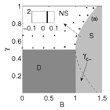
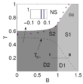
Figure 1: Theoretical $B$–$\gamma$ bifurcation diagram for $\alpha=0,\Delta\omega=1,K^{(1,2)}=0$, with (a) $A^{(1)}=A^{(2)}=1$, and (b) $A^{(1)}=1.2$, $A^{(2)}=1.0$. The different synchronization regimes are as follows: NS, no synchronization; S, synchronization with single entrainment frequency (reached via a single Hopf bifurcation); D, synchronization with two entrainment frequencies (two Hopf bifurcations); S1, both the ensembles entrained to a single frequency; S2, either of one of the ensembles synchronized with single entrainment frequency; D1, the two ensembles behave as one, with the oscillators in each ensemble entrained to either of the two distinct frequencies; D2, synchronization in both the ensembles separately with two entrainment frequencies. Regardless of symmetry, the notations S and D represent respectively single or double frequencies occurring after one or two Hopf bifurcations. The boundary between regimes NS and S/D represents $\gamma_{c+}$. The lines of $*$s represent the numerically determined bifurcation boundaries for $r>0.7$. For comparison, a numerical boundary ($\bullet$s) for $r>0.5$ is also plotted in (a). Insets show the frequency distributions (also obtained numerically) for the indicated regions; their ordinate axes represent oscillator counts in thousands. Note that the occurrence of perfect synchronization with (a) $2000$ and (b) $1000$ oscillator groups cannot be expected throughout the whole of each indicated region. The line I–II in (b) is one of the routes to synchronization discussed in Sec. V.

For a detailed analysis of the above equation, we specify sinusoidal forms for the functions $f$ and $h$ as $\{f,h\}(\theta)=\sin\theta$. Therefore the eigenvalue equation (9) becomes

$$\lambda_{\pm} = -\gamma-\bar{K}+\frac{\kappa}{4}e^{i\alpha}\pm\frac{1}{2}(\xi e^{2i\alpha}-\hat{A}(\Delta K+i\Delta\omega)e^{i\alpha}$$ (10)

$$-\Delta\omega^{2}+\Delta K^{2}+2i\Delta\omega\Delta K)^{\frac{1}{2}}-i\bar{\omega},$$

or equivalently we have

$$\lambda_{\pm}=\left\{\begin{array}[]{ll}-\bar{K}-\gamma+\frac{\kappa}{4}e^{i\alpha}\pm\frac{1}{2}(p^{2}+q^{2})^{\frac{1}{4}}e^{i\frac{1}{2}\zeta}-i\bar{\omega},&\\ \qquad\qquad\qquad\qquad\qquad\qquad\qquad p>0&\\ \\ -\bar{K}-\gamma+\frac{\kappa}{4}e^{i\alpha}\pm\frac{i}{2}(p^{2}+q^{2})^{\frac{1}{4}}e^{i\frac{1}{2}\zeta}-i\bar{\omega},&\\ \qquad\qquad\qquad\qquad\qquad\qquad\qquad p<0&\end{array}\right.$$ (16)

where $\alpha_{i}=\alpha$, $i=1,2,3$, $\kappa=A^{(1)}+A^{(2)}$, $\hat{A}=(A^{(1)}-A^{(2)})$, $\xi=(\frac{1}{4}\hat{A}^{2}+B^{2})$, $\zeta=\tan^{-1}(\frac{q}{p})$, $p=\xi\cos(2\alpha)+\hat{A}[\Delta\omega\sin{\alpha}-\Delta K\cos\alpha]-\Delta\omega^{2}+\Delta K^{2}$, $q=\xi\sin(2\alpha)-\hat{A}\Delta\omega\cos{\alpha}-\hat{A}\Delta K\sin{\alpha}+2\Delta\omega\Delta K$. The resultant bifurcation diagram is shown in Fig. 1. It is discussed in detail below, in Secs. IV.1 and IV.3. Here it is obvious that for the case when phase asymmetry is absent, when $A^{(2)}=B=0$, the characteristic equation (8) reduces to the characteristic equation of the Kuramoto model derived by Strogatz et. al. Kuramoto:84 ; Strogatz:00 .

III.1 Numerical considerations

To investigate the system numerically, we use a Runge-Kutta fourth order (RK4) routine for solving the model equations with a time step of 0.01 (we have confirmed that the results are not affected by decreasing the time step below 0.01). We take $N=1000$ in each ensemble and the initial phases of the oscillators are assumed to be equally distributed within the interval $[0,2\pi]$. As a signature of synchronization, we take the condition $Re(\lambda_{\pm})>0$ in the case of the analytic treatment. For the numerical experiment, we set $r^{(1,2)}>0.7$ for intra-ensemble synchronization in the corresponding ensembles, and a constant $\delta\psi$ for inter-ensemble synchronization as the conditions. The numerical condition for intra-ensemble synchronization, that $r^{(1,2)}>0.7$, may at first seem too strict when compared with the analytic condition that $r^{(1,2)}>0$. However, there are certain differences between analytic and numeric considerations that make this choice reasonable. Mainly, $N$ is finite for the numerical experiment, whereas analytic conditions are derived in the limit $N\rightarrow\infty$. Further, the analytic and numeric bifurcation boundaries (discussed later) are found to match quite closely for this choice of the numeric threshold for $r^{(1,2)}$. We have plotted the numerical boundary for $r=0.5$ along with $r=0.7$ in Fig. 1(a) to illustrate this.

IV Synchronization regimes

We have identified analytically the possibility of five distinct dynamical regimes Jane:08a :

• NS: the region of no synchronization or incoherence (steady state).

• S1: the region of global (inter-ensemble) synchronization, in which the oscillators of both ensembles are all entrained to the same frequency.

• S2: the region where there is synchronization within one ensemble but not the other.

• D2: the region of synchronization within both ensembles, separately and independently, with two different entrainment frequencies.

• D1: a global regime in which the two ensembles behave as one, but the oscillators within each ensemble are entrained at either one of two distinct entrainment frequencies. We will call this phenomenon inter-ensemble clustering.

Regions S2 and D1 cannot occur when coupling and noise asymmetries are absent Okuda:91 ; Montbrio:04 (see Fig. 1 (a)). In the following subsections, we will consider how these synchronization regimes are affected by coupling, noise and phase asymmetries, respectively.

IV.1 The effect of coupling asymmetry

Consider Fig. 1(b) for the case $\alpha=0$ and $K^{(1)}=K^{(2)}=0$, when $\xi-\Delta\omega^{2}>0$. If we start from the state of no synchronization (region NS), and decrease $\gamma$ for fixed $B>1$, the incoherent (steady) state becomes unstable via a single Hopf bifurcation. Thus the system enters into the region S1 from NS (crossing $\gamma_{c+}$) and the ensembles entrain to a single frequency $\Omega_{+}$. With further decrease of $\gamma$ below the $\gamma_{c-}$ line in the region D1 (in Fig. 1), a new entrainment frequency emerges through a second Hopf bifurcation. In this region, the oscillators from the two ensembles combine and form two clusters (inter-ensemble clustering) oscillating with two frequencies,

$$\Omega_{\pm} = -\mbox{Im}(\lambda_{\pm})=\pm(1/2)\left[(\xi-\Delta\omega^{2})^{2}+\hat{A}^{2}\Delta\omega^{2}\right]^{\frac{1}{4}}$$ (17)

$$\quad\times\sin{\left(\frac{1}{2}\tan^{-1}\left[\hat{A}\Delta\omega/(\xi-\Delta\omega^{2})\right]\right)}+\bar{\omega}.$$

The lines $\gamma_{c\pm}$ in Fig. 1 are obtained by imposing the condition $Re(\lambda_{\pm})=0$ in Eq. (16).

Thus in this region the order parameters $r^{(1,2)}$ either fluctuate in a quasi-periodic manner or have complicated dynamics (see Figs. 2(a) and (c)). This is because each ensemble has two clusters oscillating with different frequencies (see Figs. 2(a) and 3). Thus, the behavior of the order parameters $r^{(1,2)}$ is quite subtle. Since $r^{(1,2)}$ measure only the amount of synchronization within an ensemble, a decrease in $r^{(1,2)}$ will not necessarily mean desynchronization. Rather, for a sufficient value of the coupling parameters, a decrease in $r^{(1,2)}$ represents a signature of inter-ensemble synchronization: clustering corresponds to the occurrence of desynchronization within an ensemble because some of its oscillators tend to synchronize with the other ensemble.

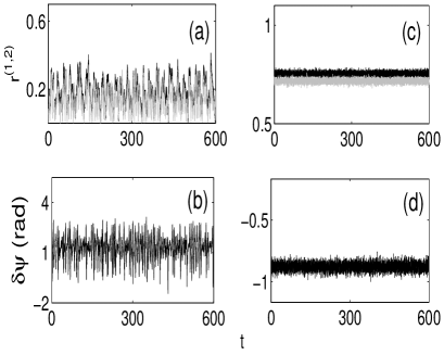
Figure 2: Time variations of the coherence parameters $r^{(1)}$ (grey), $r^{(2)}$ (black) and the phase difference $\delta\psi$, as obtained from numerical simulations. Parameter values are: (a), (b) $B=1$, $\alpha=0.23$ and (c), (d) $B=1$, $\alpha=0.47$ corresponding to regions D1 and D2 respectively of Fig. 1(b) as traveling along the line $I-II$. Note that in region D1 the order parameters display no synchronization.

Again looking at Fig. 1(b), when $B<1$, a decrease in $\gamma$ takes the system from region NS to region S2 by crossing the line $\gamma_{c+}$ through a single Hopf bifurcation. Further decrease in $\gamma$ causes the system to cross the line $\gamma_{c-}$ and, via another Hopf bifurcation, enter into region D2 where there are two entrainment frequencies $\Omega_{\pm}$. The latter can be calculated from Eq. (16). In region S2, intra-ensemble synchronization can occur in either one of the ensembles, depending upon whether $A^{(1)}$ or $A^{(2)}$ is greater; in Fig. 1(b), since $A^{(1)}>A^{(2)}$, synchronization occurs in the first ensemble with the second ensemble remaining incoherent. Note that, on increasing $B$ (for fixed $\gamma$) while in region S2, the condition $\xi-\Delta\omega^{2}<0$ is violated and the ensembles enter into the phase-locked region S1. In region D2, the ensembles synchronize separately to two the locking frequencies (unlike region D1 where the ensembles combine and synchronize to two locking frequencies given by Eq. (17)).

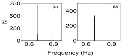
Figure 3: The distribution of frequencies in region D1 for the same parameter values as in Fig. 2(a): (a) first ensemble; (b) second ensemble. The splitting of the first frequency component into two almost indistinguishable sub-components corresponds to a discrepancy between numerics and analytics, attributable to approximations (see text) made in the former.

The corresponding $(B-\gamma)$ bifurcation diagram for the case $A^{(1)}$=$A^{(2)}$ is plotted in Fig. 1(a) to show the difference between these two cases. Region D represents intra-ensemble synchronization which occurs through a degenerate Hopf bifurcation (similar to the route to D2) with entrainment frequencies $\Omega_{\pm}=\mp(1/2)(\Delta\omega^{2}-B^{2})^{\frac{1}{2}}+\bar{\omega}$ and S represents inter-ensemble synchronization through a single Hopf bifurcation (similar to the route to S1) with same frequency $\Omega=\bar{\omega}$. Note that regions S2 and D1 cannot arise for the symmetric coupling case and that these two synchronization regimes are therefore induced by coupling asymmetry.

The presence of two entrainment frequencies in region D1 can be seen by looking at the frequencies into which all the individual oscillators are grouped as shown in Fig. 3 (since the order parameters do not reveal this synchronization phenomenon). The inter-ensemble clustering that occurs in this case is quite different from the formation of clusters in a single ensemble Kuramoto:84 ; Tass:97 ; Kouomou:03 – here the oscillators in two different ensembles combine and form clusters. The occurrence of this phenomenon provides a new insight into possible ways of controlling synchronization in more realistic situations (considering asymmetry) like neural networks where some neurons from one ensemble (say cortex) tend to synchronize with other ensemble (say thalamus) creating desirable (temporal coding) or undesirable effects (as in the case of epileptic seizures). For instance, in a thalamocortical model of the neuronal synchronization mechanisms during anæsthesia Jane:08b , we found that the transition from deep to light anæsthetized state occurs as a result of a fraction of the thalamic neurons entering into synchronization with the cortex, at the same time losing synchronization within its own ensemble. The clustering that occurs in this case is desirable in the sense that it favours coding of sensory information and helps the brain to resist the effects of anæsthesia and successfully maintain consciousness and cognition. Without coupling asymmetry, these phenomena would not occur.

IV.2 The effect of noise asymmetry

It is well known that real physical systems are in general subject to noise. Here, we regard as “noise” any kind of random fluctuation in the system, whether originating internally or externally. Synchronization effects, induced and modified noise, are one of particular interest He:03 ; Goldobin:05 ; Nakao:07 ; Kawamura:07 ; Kawamura:08 .

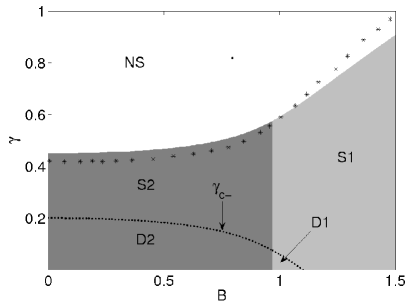
Figure 4: Theoretical $B$–$\gamma$ bifurcation diagram for asymmetric noise with $A^{(1)}=A^{(2)}=1$, $\Delta K=0.25$ with $K^{(1)}=0.3$ and $K^{(2)}=0.05$, $\Delta\omega=1$. Note that the synchronization regimes S2 and D1 emerge in the presence of noise asymmetry even for symmetric coupling (cf. Fig. 1(a)).

When asymmetric noise in introduced into a system with asymmetric coupling, the bifurcation regimes remain the same in the presence of coupling and phase asymmetries. There may be changes in the boundaries of the respective regions and their entrainment frequencies. However, for the case of symmetric coupling, asymmetric noise can induce the phenomenon of global clustering. We have already seen in Sec. IV.1 that inter-ensemble clustering phenomena (region D1) cannot occur in a system with symmetric coupling and symmetric noise. Fig. 5 plots the individual oscillator phases, determined numerically, indicating the transition from S1 to D1 induced by noise asymmetry. When $A^{(1)}=A^{(2)}=1.4$, $B=1$, $\gamma=0.05$ and $\Delta K=0$ the system is in region S (corresponding to Fig. 1 (a)) where synchronization occurs in both the ensembles with one entrainment frequency. This can be seen from the top panel of Fig. 5 where oscillators from both ensembles lock to form a single major cluster. On the other hand, when $\Delta K=0.25$, the combined system of the two ensembles synchronize to two main clusters, each of which comprises a fraction of the oscillators from both ensembles (see Fig. 5 (bottom)), representing region D1. Thus it is becomes obvious that asymmetric noise can in some ways imitate the effects of asymmetric coupling when the latter is absent.

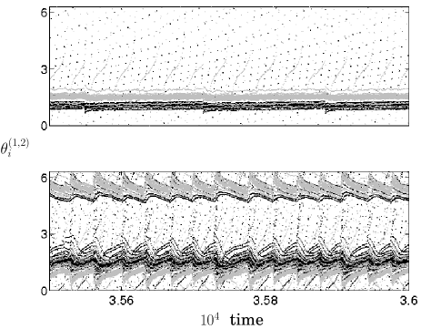
Figure 5: Time evolution of the oscillator phases in the first (grey) and second (black) ensembles. Parameter values are $A_{1}=A_{2}=1.4$, $B=1$, $\gamma=0.05$, and either $\Delta K=0$, with $K^{(1)}=0.2$ and $K^{(2)}=0.2$ (top) or $\Delta K=0.25$, with $K^{(1)}=0.2$ and $K^{(2)}=-0.05$ (bottom). Thus the top and the bottom panels represent respectively the synchronization regions S and D1, induced by noise asymmetry.

The S2 region also appears in this case, induced by noise asymmetry. Here too, depending upon whether $\Delta K$ is positive or negative, synchronization occurs either in the second or the first ensemble respectively, similar to the case when region S2 arises in the presence of coupling asymmetry. Thus noise asymmetry plays a similar role to coupling asymmetry for the symmetric coupling case, and the $(B-\gamma)$ bifurcation diagrams 1(b) and 4 look similar. Fig. 6 depicts the results of numerical investigation of all the synchronization regimes in the presence of noise asymmetry corresponding to the analytical bifurcation diagram in Fig. 4. In contrast, for symmetric noise the dynamics is unaffected, no matter whether coupling and phase asymmetries are present or absent. The only difference is that the incoherent state becomes unstable for larger values of the critical parameters as one increases noise intensity.

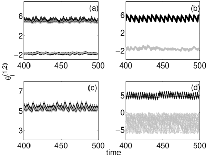
Figure 6: Noise asymmetry-induced synchronization regimes obtained numerically for the case of symmetric coupling. Black and grey lines represent the time evolution of the oscillator phases in the first and second ensembles respectively, for the same parameter values as in Fig. 4 and: (a) $B=1$, $\gamma=0.1$; (b) $B=0.5$, $\gamma=0.1$; (c) $B=1.2$, $\gamma=0.4$; and (d) $B=0.6$, $\gamma=0.4$. Panels (a)–(d) represent the synchronization regimes D1, D2, S1, S2 respectively.

IV.3 The effect of phase asymmetry

For the case $\alpha\neq 0$, the inter-ensemble regions D1 and S1 shrink as $\alpha$ increases, whereas the intra-ensemble synchronization region S2 expands, as shown in Fig. 7. This means that finite phase asymmetry reduces the probability of inter-ensemble synchronization (note reduced S1 and D1 regions in Fig. 7) and mostly allows only intra-ensemble synchronization of one or both of the ensembles. For a given set of parameters, on increasing $\alpha$ from 0, the following condition is satisfied

$$\xi\cos(2\alpha)+\hat{A}\Delta\omega\sin{\alpha}-\Delta\omega^{2}>0$$ (18)

up to a critical value of $\alpha=\alpha_{j}$ given by

$$\alpha_{j}=\sin^{-1}\bigg{[}\frac{\hat{A}\Delta\omega\pm(8\xi^{2}-\Delta\omega^{2}(\hat{A}^{2}+B^{2}))^{\frac{1}{2}}}{4\xi}\bigg{]},$$

where again, for a given set of parameters, there can only be one value of $\alpha$ that satisfies $0<\alpha\leq\pi/2$. Upon crossing $\alpha_{j}$, the condition (18) is violated and the following condition is satisfied $\xi\cos(2\alpha)+\hat{A}\Delta\omega\sin{\alpha}-\Delta\omega^{2}<0$.

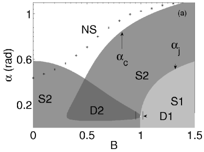
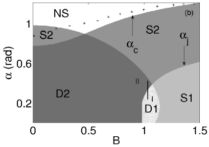
Figure 7: Theoretical $B$–$\alpha$ bifurcation diagram for (a) $A^{(1)}=1.2,A^{(2)}=1$, (b) $A^{(1)}=1.8,A^{(2)}=1.4$ and $\Delta\omega=1,\gamma=0.5$. The line of $*$s represents the numerically obtained bifurcation boundary between the synchronized and incoherent states. Greatly reduced S1 and D1 regions occur due to the presence of phase asymmetry. The discrepancy between numerical and analytic boundaries is discussed in the text.

As a result, when $\alpha>\alpha_{j}$ the inter-ensemble synchronization breaks down and the system enters into a state of intra-ensemble synchronization. Thus as one travels from S1 (D1) to S2 (D2) across $\alpha_{j}$ the combined synchronization with single (double) frequency breaks between the ensembles and independent synchronization with single (double) frequency regime appears. Region S2, unlike region S in Fig. 1 (a), embraces two states (i) synchronization in ensemble 1 with ensemble 2 incoherent and (ii) synchronization in ensemble 2 with ensemble 1 incoherent, but does not distinguish between them.

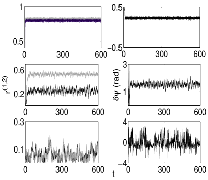
Figure 8: The coherence parameters $r^{(1)}$ (grey) and $r^{(2)}$ (black), and the phase difference $\delta\psi$, plotted as functions of time, obtained from numerical simulations. Parameter values were: top panel, $B=0.7,\alpha=0.2$; middle panel, $B=0.7,\alpha=\pi/4$ (near $\alpha_{c}$); and bottom panel, $B=0.7,\alpha=1.2$ ($\alpha>\alpha_{c}$), corresponding to regions D2 near the NS/S2 boundary and NS respectively (see Fig. 7(a)).

Further, there is a critical value of $\alpha=\alpha_{c}$ above which the collective oscillations disappear and the incoherent state becomes stabilized (see Figs. 7 and 8). Thus by reducing the chances of occurrence of inter-ensemble synchronization and favoring intra-ensemble synchronization, phase asymmetry plays a crucial role in determining the route to synchronization. Thus, for instance, in a particular problem, if one wants to have (avoid) the phenomenon of inter-ensemble clustering (region D1) then it is obvious that phase asymmetry should be absent (finite, large).

The discrepancy between the numerically and analytically obtained boundaries in Fig. 7 is attributable to the influence of phase asymmetry. This affects region S2 which is large here (cf. Fig. 1(b) where both S2 and the discrepancy are smaller) and it changes the thresholds for $r^{(1)}$ and $r^{(2)}$. Note that neither numerics nor analytics provides an exact result. The analytic boundary is obtained from the condition $r^{(1,2)}>0$ and refers to the limit of infinitely many oscillators. For numerics, the (asterisked) boundary is obtained from the condition $r^{(1,2)}>0.7$ and refers to a finite number of oscillators.

IV.4 Stability of the fully synchronized states in the limit $\gamma=0$

In this subsection we focus on the noise-free case with a frequency distribution that has an infinitely sharp peak. In this case, the dynamics is reduced to that of two ensembles of identical oscillators (the oscillators within the ensembles are identical while the ensembles themselves are non-identical). Now the $\delta\psi$ corresponding to intra-ensemble synchronization can be obtained from Eq. (1) as

$$\delta\psi=\sin^{-1}[(\Delta\omega-\hat{A}\sin\alpha)/2B\cos\alpha].$$

A linear stability analysis of Eq. (1) then gives $N-1$ degenerate eigenvalues for each ensemble, namely

$$\lambda_{\pm}=-A^{(1,2)}\cos\alpha-B\cos(\pm\delta\psi+\alpha)<0,$$

that characterize the stability of the intra-ensemble synchronized states of ensembles 1 and 2 respectively. In addition, two eigenvalues $\lambda_{0}=0$ and $\lambda_{c}=-2B\cos\alpha\cos\delta\psi$ characterize the stability of inter-ensemble synchronization. Hence the transition between inter-ensemble and intra-ensemble synchronization states occurs at the following bifurcation point

$$B_{c}=(\Delta\omega-\hat{A}\sin\alpha)/2\cos\alpha.$$

Note that $\delta\psi$ varies from $-\pi/2$ to $\pi/2$ as $\alpha$ increases. For $\alpha<\alpha_{h}$ (not shown in figures), the stability condition is satisfied by both ensembles and so intra-ensemble synchronization occurs in both ensembles. When $\alpha\geq\alpha_{h}$ the stability condition is violated by either one of the ensembles and at that point a Hopf bifurcation occurs. As a consequence, intra-ensemble synchronization occurs in one of the ensembles. For the case $A^{(1)}=A^{(2)}$, when $\delta\psi$ varies from $\pi/2$ to $0$ for increasing $\alpha$ and when $\alpha\geq\alpha_{h}$ the stability condition is violated by the first ensemble. On the other hand, when $\delta\psi$ varies from $0$ to $-\pi/2$ with increasing $\alpha$, the stability condition is violated by the second ensemble above $\alpha_{h}$.

V Routes to synchronization

Given that the system possesses distinct synchronization regimes, it is of interest to investigate the routes it follows to synchronization. As one would expect, the route depends on the coupling, noise and phase asymmetries. In particular, in the presence of coupling asymmetry, we have identified the following routes Jane:08a , grouped into the two different cases $\alpha=0$ and $\alpha\neq 0$, and assuming that we increase the inter-ensemble coupling parameter $B$ keeping all the other parameters fixed. When $\alpha=0$ we find that there are at least three typical routes:

1. The oscillators in the ensembles pass from the synchronization regime D2 through D1 to the region S1. Thus when the ensembles are synchronized separately, increasing $B$ results in inter-ensemble clustering which then leads to inter-ensemble synchronization or phase locking between the ensembles. This route is represented by line I-II of Fig. 1(b).

2. There is also a possibility that when the ensembles are synchronized separately and when $B$ is increased, the intra-ensemble synchronization be destroyed in one of the ensembles, which on further increase of $B$, leads to phase-locking between the ensembles. Thus when the system is in region D2 increasing $B$ causes the system to pass through the region S2 to region S1. Inter-ensemble clustering does not occur in this route.

3. If the ensembles are initially not synchronized (that is in region NS), then increasing $B$ can cause phase-locking of the ensembles directly. Thus the system can pass directly from region NS to to S1. This route is characteristic of the case $\alpha=0$ and cannot occur in the presence of phase asymmetry.

In the presence of phase asymmetry, i.e. $\alpha\neq 0$, the ensembles can follow any of the following routes to synchronization

1. The ensembles pass from region D2 through D1 to S1. This route is similar to route 1 that occurs for the case $\alpha=0$. Note that when $A^{(1)}=A^{(2)}$ or $\Delta\omega=0$ only one entrainment frequency exists below $\gamma_{c-}$ and therefore this route does not occur for either cases (due to the non-occurrence of region D1).

2. The ensembles pass from region D2 through S2 to S1. This route does not incorporate the state of inter-ensemble clustering.

3. When the ensembles are synchronized separately (in region D2), increasing $B$ causes the disruption of synchronization in one of the ensembles leading to synchronization in the other ensemble (region S2). Thus the ensembles pass from region D2 to S2. This route is characteristic of phase asymmetry and cannot occur for the case $\alpha=0$.

4. If the ensembles are not synchronized, increasing $B$ will result in synchronization in either one of the ensembles. Thus the ensembles pass from regions NS to S2 (unlike NS to S1 in the absence of phase asymmetry).

Knowledge of these routes to synchronization is obviously important for the control of synchronization in real systems.

VI Discussion and conclusions

One might intuitively suggest that the synchronization phenomena induced by coupling and noise asymmetries could also be obtained by choosing a sufficiently large difference between the mean frequencies of the two ensembles. However, the synchronization phenomena corresponding to the D1 and S2 regions can only be explained by introducing either coupling or noise asymmetries. As an illustration let us consider the eigenvalue for the noise-free case without coupling and phase asymmetries for $\Delta\omega^{2}>B^{2}$

$$\lambda_{\pm}=-\gamma+\frac{A}{2}\pm i\frac{1}{2}\sqrt{\Delta\omega^{2}-B^{2}}-i\bar{\omega}.$$

For this case, the intra-ensemble synchronization takes place simultaneously in the two ensembles since the curves $\gamma_{c+}$ and $\gamma_{c-}$ coincide when $Re(\lambda_{\pm})$ becomes positive. Although there occur two Hopf bifurcations, they happen to be one and the same and hence one will not be able to explain the synchronization region S2. A similar problem occurs also with the D1 synchronization regime for $\Delta\omega^{2}<B^{2}$. Therefore we must conclude that the introduction of coupling/noise asymmetries are crucial to account for certain synchronization phenomena and can never be replaced by the introduction of large difference between the mean frequencies of the two ensembles.

It is therefore essential to take account of possible asymmetry while attempting to model natural systems. Certain phenomena, like those discussed here, are attributable to asymmetries in the interactions.

In this paper, we have investigated the role played by coupling, noise and phase asymmetries in two coupled phase oscillator ensembles. We have identified a global clustering phenomenon that may be characteristic of either the coupling or the noise asymmetry when the other is absent. Phase asymmetry reduces the likelihood of global clustering and also introduces new routes that are characteristic of itself. Thus phase asymmetry controls the routes to inter-ensemble synchronization. The phenomenon of inter-ensemble clustering that is characteristic of coupling asymmetry is found to occur even for symmetrically coupled systems if noise asymmetry is present. Thus noise asymmetry is found to complement the effect of coupling asymmetry when the latter is absent.

We therefore conclude that, in modeling real systems where synchronization arises, explicit consideration should be given to the effect of possible asymmetries in coupling, noise, and phase.

References

- (1) J. Buck, and E. Buck, Science 159, 1319 (1968).
- (2) C. S. Peskin, Mathematical Aspects of Heart Physiology (Courant Institute of Mathematical Sciences, New York, (1975).
- (3) I. Z. Kiss, Y. M. Zhai, J. L. Hudson, Phys. Rev. Lett. 88, 238301 (2002).
- (4) I. Z. Kiss, Y. M. Zhai, J. L. Hudson, Science 296, 1676 (2002).
- (5) D. Hansel, and H. Sompolinsky, Phys. Rev. Lett 68, 718 (1992).
- (6) P. C. Bressloff, Phys. Rev. E 60, 2160 (1999).
- (7) D. Golomb, D. Hansel, and G. Mato, in Neuroinformatics, edited by F. Moss and S. Gielen, Handbook of Biological Physics Vol. 4 (Elsevier, Amsterdam, 2001), pp.887–968.
- (8) T. J. Walker, Science 166, 891 (1969).
- (9) A. T. Winfree, J. Theor. Biol. 16, 15 (1967).
- (10) Y. Kuramoto, Chemical Oscillations, Waves, and Turbulence (Springer-Verlag, Berlin, 1984).
- (11) S. H. Strogatz, Physica D 143, 1 (2000).
- (12) S. H. Strogatz, Nature 410, 268 (2001).
- (13) A. Pikovsky, M. Rosenblum, and J. Kurths, Synchronization – A Universal Concept in Nonlinear Sciences (Cambridge University Press, Cambridge, 2001).
- (14) Jane H. Sheeba, V. K. Chandrasekar, A. Stefanovska, and P. V. E. McClintock, Phys. Rev. E 78, 025201(R) (2008).
- (15) A. T. Winfree, The Geometry of Biological Time (Springer, Berlin, 1980).
- (16) A. Pikovsky, M. Rosenblum, and J. Kurths, Europhys. Lett. 34, 165 (1996).
- (17) N. F. Rulkov, Phys. Rev. Lett 86, 183 (2001).
- (18) H. Haken, Advanced Synergetics: Instability Hierarchies of Self–Organizing Systems (Springer, Berlin, 1993).
- (19) Z. Néda, E. Ravasz, Y. Brechet, T.Vicsek, and A.L. Barabasi, Nature (London) 403, 849 (2000).
- (20) D. Topaj, W.-H. Kye, and A. Pikovsky, Phys. Rev. Lett. 87, 074101 (2001).
- (21) B. Blasius, E. Montbrio, J. Kurths, Phys. Rev. E. 67, 035204(R) (2003).
- (22) E. Montbrio and B. Blasius, Chaos 13, 291 (2003).
- (23) B. Blasius, Phys. Rev. E. 72, 066216 (2005).
- (24) B. R. Trees, V. Saranathan, D. Stroud, Phys. Rev. E 71, 016215 (2005).
- (25) F. Rogister, R. Roy, Phys. Rev. Lett. 98 104101 (2007).
- (26) C. Schafer, M. G. Rosenblum, J. Kurths and H. H. Abel, Nature 392 239 (1998).
- (27) M. B. Lotrič and A. Stefanovska, Physica A 283 451 (2000).
- (28) W. Singer, Nature 397, 6718 (1999).
- (29) W. Singer, Neuron 24 49 (1999).
- (30) P. Fries, Trends. Cogn. Sci. 9 474 (2005).
- (31) Y. Yamaguchi, N. Sato, H. Wagatsuma, Z. Wu, C. Molter and Y. Aota, Curr. Opin. Neurobiol. 17, 197 (2007).
- (32) Jane H. Sheeba, A. Stefanovska, and P. V. E. McClintock, Biophys. J. 95, 2722 (2008).
- (33) J. A. Goldberg, T. Boraud, S. Maraton, S. N. Haber, E. Vaadia, and H. Bergman, J. Neurosci. 22, 4639 (2002).
- (34) L. Timmermann, J. Gross, M. Dirks, J. Volkmann, H. Freund and A. Schnitzler, Brain 126, 199 (2003).
- (35) B. Percha, R. Dzakpasu, and M. Zochowski, Phys. Rev. E. 72, 031909 (2005).
- (36) M. Zucconi, M. Manconi, D. Bizzozero, F. Rundo, C. J. Stam, L. Ferini-Strambi, R. Ferri, Neurol. Sci. 26 199 (2005).
- (37) A. Stefanovska and M. Bračič, Contemp. Phys. 40 31 (1999).
- (38) M. Paluš and A. Stefanovska, Phys. Rev. E 67 055201 (2003).
- (39) B. Musizza, A. Stefanovska, P. V. E. McClintock, M. Paluš, J. Petrovčič, S. Ribarič, F. F. Bajrović, J. Physiol. (London) 580, 315 (2007).
- (40) H. Daido, and K. Nakanishi, Phys. Rev. Lett. 93, 104101 (2004).
- (41) H. Daido, and K. Nakanishi, Phys. Rev. Lett. 96, 054101 (2006).
- (42) H. Daido, and K. Nakanishi, Phys. Rev. E. 75, 056206 (2007).
- (43) A. Sherman, J. Rinzel, Proc. Natl. Acad. Sci. U.S.A. 89, 2471 (1992).
- (44) H. Fukuda, N. Nakamichi, M. Hisatsune, H. Murase, and T. Mizuno, Phys. Rev. Lett. 99, 098102 (2007).
- (45) P. R. Roelfsema, A. K. Engel, P. Konig and W. Singer, Nature 385, 6612 (1997).
- (46) K. Okuda and Y. Kuramoto, Prog. Theor. Phys. 86, 1159 (1991).
- (47) E. Montbrio, J. Kurths, and B. Blasius, Phys. Rev. E 70, 056125 (2004).
- (48) P. Tass, Phys. Rev. E 56, 2043 (1997).
- (49) Y. C. Kouomou and P. Woafo, Phys. Rev. E 67, 046205 (2003).
- (50) D. He, P. Shi, and L. Stone, Phys. Rev. E 67, 027201 (2003).
- (51) Denis S. Goldobin, and A. Pikovsky, Phys. Rev. E 71, 045201(R) (2005).
- (52) H. Nakao, K. Arai, and Y. Kawamura, Phys. Rev. Lett. 98, 184101 (2007).
- (53) Y. Kawamura and H. Nakao, Phys. Rev. E 75, 036209 (2007).
- (54) Y. Kawamura, H. Nakao, K. Arai, H. Kori and Y. Kuramoto Phys. Rev. Lett. 101, 024101 (2008).