On quantum optical properties of single-walled carbon nanotube

Abstract

We study quantum optical properties of the single-walled carbon nanotube (SWCNT) by introducing the effective interaction between the quantized electromagnetic field and the confined electrons in the SWCNT. Our purpose is to explore the quantum natures of electron transport in the SWCNT by probing its various quantum optical properties relevant to quantum coherence, such as the interference of the scattered and emitted photons, and the bunching and anti-bunching of photons which are characterized by the higher order coherence functions. In the strong field limit, we study the interband Rabi oscillation of electrons driven by a classical light. We also investigate the possible lasing mechanism in superradiation of coherent electrons in a SWCNT driven by a light pump or electron injection, which generate electron population inversion in the higher energy-band of SWCNT.

I INTRODUCTION

Carbon nanotubes (CNTs) have been under great focus these years because of their promising thermal and electrical conductivities, and other unusual features that may lead to new applications Carbon1 ; Carbon2 ; Carbon3 . In recent years, individual single-walled carbon nanotubes (SWCNTs) have experimentally become available for the design of future quantum devices SWCNT1 ; SWCNT2 ; SWCNT3 ; SWCNT4 . Through putting such a SWCNT between electrodes while maintaining a low contact resistance, novel CMOS devices can be made from this novel material field1 ; field2 ; field3 . Surpassing the current silicon-based CMOS devices, CNT-based CMOS devices appear to have the potential for wide applications. To this end, a broad research is required on various aspects of its characteristics beforehand.

The conventional investigation for a new material is to explore its photoluminescence optical1 ; optical2 ; optical3 ; optical4 ; optical5 ; optical6 ; optical7 ; optical8 ; optical9 . We usually study the characteristic spectroscopy of the light scattered by or emitted from this material. Meanwhile, since ballistic transport–a motion of electrons with negligible electrical resistivity due to scattering in the process of transportation–happens in a SWCNT at low temperature field1 ; ballistic , SWCNT should be treated beyond the classical scenario, and pure quantum effects should be taken into account. As a result, not only should the classical optical properties (e.g., the intensity, the spectrum, etc,) of the SWCNT be considered, but also the quantum optical properties (e.g., the bunching and antibunching phenomena, etc,) need to be studied in details. In this paper we develop a fully quantum approach for the SWCNT-light interaction to address the quantum effects relevant to the higher order quantum coherence. Our investigation is oriented by the great potential to implement the quantum optical devices based on current carbon nanotube technology, which works in the quantum regime, or at a level of single quantum state.

Starting from the minimal coupling theorem, we derive the effective Hamiltonian of the SWCNT interacting with a fully quantized light field. The interband Rabi oscillation is first studied for the light field whose intensity is sufficiently strong to be treated classically. We explore the full quantum features of the transporting electron in the SWCNT which is displayed by its quantum optical properties. To this end, we quantize the light field interacting with the confined electrons in SWCNT, and calculate and analyze the higher order coherence functions of the photons scattered or emitted from the SWCNT. It is shown that the total population inversion of electrons, the first order and the second order coherence functions strongly depends on the chiral vector of the SWCNT, while this dependence does not exist in the generic graphene. Additionally, the anti-bunching feature of the light field is predicted with detailed calculations based on the long time approximation. A similar discovery has been made in an experiment ballistic , but to our best knowledge no microscopic theoretical explanation has been given.

This paper is organized as follows. In Sec. II, the interaction between the quantized light field and the SWCNT based on the tight binding approach is derived from the the minimal coupling theorem. In Sec. III, we study the interband Rabi oscillation of the electrons in the SWCNT induced by strong light when the driving light can be treated classically, the reason of which is generally proved in App. A. The interference of the scattered light from the SWCNT and the second order correlation of the emitted photons are investigated in Sec. IV and Sec. V, respectively. Additionally, the possible lasing mechanism of the SWCNT through a light pump or electron injection is discussed in Sec. VI. The conclusions are presented in Sec. VII.

II MODEL SETUP

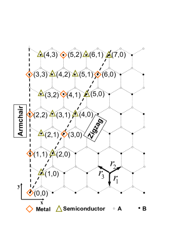
Figure 1: Schematic illustration of the $2$-D hexagonal lattice of the SWCNT, which contain two sets of sublattices A and B. The pair numbers $(n,m)$ denotes the chiral vector.

The difference between carbon nanotubes and graphene is that carbon nanotubes allow merely discrete wave vectors along their specific chiral vector while graphene allows continuous ones, as long as we neglect such effects as distortion of the lattice in carbon nanotubes. Thus, to simplify the modeling of the system in consideration, we can take the tight banding model of graphene into account, and then apply discrete wave vector restriction to demonstrate the properties of the nanotube. The honeycomb lattice of graphene is divided into two triangular sublattices $A$ and $B$  (see Fig. 1). Here, the chiral vector of the SWCNT is denoted as a pair of numbers $(n,m).$ The discrete wave vectors for carbon nanotubes will be directly introduced by boundary conditions later.

Since electrons in graphene approximately hop from one site to the nearest neighbor one, a tight binding model

$$H_{e}=-J\sum\limits_{\mathbf{r}\in A}\sum_{\alpha=1}^{3}[a^{\dagger}(\mathbf{r})b(\mathbf{r}+\mathbf{r}_{\alpha})+h.c.]$$ (1)

is applied to describe the motion of the electrons in the graphene. Here, $J$ is the hopping constant; $a\ (a^{\dagger})$ and $b\ (b^{\dagger})$ annihilates (creates) an electron at sublattice $A$ and $B$, respectively. And $\mathbf{r}_{\alpha}$ $(\alpha=1,2,3)$ are the real space vectors pointing from one site to its nearest neighbors. Usually they are chosen as

$$\mathbf{r}_{1} = \frac{l}{\sqrt{3}}(0,-1),$$ (2a)

$$\mathbf{r}_{2} = \frac{l}{\sqrt{3}}(\frac{\sqrt{3}}{2},\frac{1}{2}),$$ (2b)

$$\mathbf{r}_{3} = \frac{l}{\sqrt{3}}(-\frac{\sqrt{3}}{2},\frac{1}{2})$$ (2c)

, and are schematically plotted in Fig. 1. Here, $$l A B.$$ is the lattice constant of both the triangular sublattice and

To diagonalize the above tight banding  Hamiltonian,  a 2D Fourier transformation

$$c_{\mathbf{k}}=\sum\limits_{\mathbf{r}\in C}c(\mathbf{r})e^{-i\mathbf{k}\cdot\mathbf{r}},(c=a\text{ or }b,C=A\text{ or }B).$$ (3)

is used to give the momentum space- representation of the Hamiltonian (1)

$$H_{e}=\sum\limits_{\mathbf{k}}\left(\Phi_{\mathbf{k}}a_{\mathbf{k}}^{\dagger}b_{\mathbf{k}}+h.c.\right).$$ (4)

Here the transition energy $\Phi_{\mathbf{k}}\equiv-J\sum\limits_{\mathbf{\delta}\in\{\mathbf{r}_{\alpha}\}}e^{i\mathbf{k}\cdot\mathbf{\delta}}$ is a summation over all the directions of nearest neighbors. It is explicitly written as

$$\Phi_{\mathbf{k}}=-Je^{i\frac{k_{x}l}{\sqrt{3}}}\left(1+2\cos\frac{k_{y}l}{2}e^{-i\frac{\sqrt{3}k_{x}l}{2}}\right).$$ (5)

and corresponds to the transition of electrons between two sublattices $A$ and $B$. Further, this Hamiltonian (4) is diagonalized as

$$H_{e}=\sum\limits_{\mathbf{k}}E_{\mathbf{k}}\left(\alpha_{\mathbf{k}}^{\dagger}\alpha_{\mathbf{k}}-\beta_{\mathbf{k}}^{\dagger}\beta_{\mathbf{k}}\right)$$ (6)

through a unitary transformation

$$\alpha_{\mathbf{k}} = \frac{1}{\sqrt{2}}\left(e^{-i\varphi_{\mathbf{k}}}a_{\mathbf{k}}+e^{i\varphi_{\mathbf{k}}}b_{\mathbf{k}}\right),$$ (7a)

$$\beta_{\mathbf{k}} = \frac{1}{\sqrt{2}}\left(e^{-i\varphi_{\mathbf{k}}}a_{\mathbf{k}}-e^{i\varphi_{\mathbf{k}}}b_{\mathbf{k}}\right).$$ (7b)

Here, the single particle spectrum is

$$E_{\mathbf{k}}=J\sqrt{1+4\cos(\frac{k_{x}l}{2})\left[\cos(\frac{\sqrt{3}}{2}k_{y}l)+\cos(\frac{k_{x}l}{2})\right]}$$ (8)

with the phase $\varphi_{\mathbf{k}}$ determined by

$$\tan 2\varphi_{\mathbf{k}}=-\frac{2\cos\left(k_{x}l/2\right)\sin\left(\sqrt{3}k_{y}l/2\right)}{1+2\cos\left(k_{x}l/2\right)\cos\left(\sqrt{3}k_{y}l/2\right)}.$$ (9)

We have to point out that the energy $2E_{\mathbf{k}}$ of  single electron excitation actually has six Dirac points on the six vertices of the first Brillouin Zone in the momentum space. It has been discovered that in the vicinity of Dirac points, the effective motion of the electrons accords with the relativistic theory, which is described by the massless or massive Dirac equation with an effective light velocity .

In order to study the quantum optical properties of the nanotubes, it is necessary to introduce a quantized light field

$$H_{p}=\sum\limits_{\mathbf{q}}\hbar\Omega_{\mathbf{q}}d_{\mathbf{q}}^{\dagger}d_{\mathbf{q}},$$ (10)

where $\Omega_{\mathbf{q}}$ is the frequency of photons with momentum $\mathbf{q}$. $d_{\mathbf{q}}^{\dagger}$ and $d_{\mathbf{q}}$ creates and annihilates a photon with momentum $\mathbf{q},$ respectively. We choose $\hbar=1$ and only one polarization direction for each mode of light denoted by $\mathbf{q}$ in the following discussions.

The interaction between the carbon nanotube and the light field is obtained according to the minimal coupling principle of electromagnetic field. By replacing the mechanical momentum of the electrons with canonical ones and neglecting the multi-photon interactions, the interaction Hamiltonian is obtained as

$$H_{I}=-\frac{e}{mc}\sum\limits_{\mathbf{k},\mathbf{q}}\mathbf{k}\cdot\mathbf{A}_{\mathbf{q}}\left(a_{\mathbf{k}}^{\dagger}+b_{\mathbf{k}}^{\dagger}\right)\left(a_{\mathbf{k-q}}+b_{\mathbf{k-q}}\right).$$ (11)

Here, the vector potential of the quantized light field is

$$\mathbf{A}_{\mathbf{q}}=-i\sqrt{\frac{1}{2\epsilon_{0}V\Omega_{\mathbf{q}}}}\mathbf{e}_{\mathbf{q}}\left(d_{\mathbf{q}}-d_{-\mathbf{q}}^{\dagger}\right),$$ (12)

where $\mathbf{e}_{\mathbf{q}}$ is the unit polarization vector of mode $\mathbf{q}.$ $\epsilon_{0}$ is the vacuum electric permittivity and $V$ is the volume effectively occupied by the light field.

So far, we have obtained the quantized mode of the SWCNT interacting with a light field, whose Hamiltonian is $H=H_{e}+H_{p}+H_{I}$, with

$$H_{e} = \sum\limits_{\mathbf{k}}E_{\mathbf{k}}\left(\alpha_{\mathbf{k}}^{\dagger}\alpha_{\mathbf{k}}-\beta_{\mathbf{k}}^{\dagger}\beta_{\mathbf{k}}\right),$$ (13a)

$$H_{p} = \sum\limits_{\mathbf{q}}\hbar\Omega_{\mathbf{q}}d_{\mathbf{q}}^{\dagger}d_{\mathbf{q}},$$ (13b)

$$H_{I} = \sum_{\mathbf{k},\mathbf{q}}D_{\mathbf{k,q}}\left(d_{\mathbf{q}}\alpha_{\mathbf{k}}^{\dagger}\beta_{\mathbf{k}-\mathbf{q}}+h.c.\right),$$ (13c)

where we have made the rotating wave approximation to eliminate the fast varying terms, such as $$d_{-\mathbf{q}}^{\dagger}\alpha_{\mathbf{k}}^{\dagger}\beta_{\mathbf{k-q}} d_{\mathbf{q}}\beta_{\mathbf{k}}^{\dagger}\alpha_{\mathbf{k-q}} d_{-\mathbf{q}}^{\dagger}\alpha_{\mathbf{k}}^{\dagger}\alpha_{\mathbf{k-q}} d_{\mathbf{q}}\alpha_{\mathbf{k}}^{\dagger}\alpha_{\mathbf{k-q}} d_{-\mathbf{q}}^{\dagger}\beta_{\mathbf{k}}^{\dagger}\beta_{\mathbf{k-q}} d_{\mathbf{q}}\beta_{\mathbf{k}}^{\dagger}\beta_{\mathbf{k-q}} D_{\mathbf{k,q}}$$, , , , , and , and the coefficient for electron-photon interaction is

$$D_{\mathbf{k,q}} = -\frac{e}{\sqrt{2}mc}\mathbf{k}\cdot\mathbf{e}_{\mathbf{q}}\sqrt{\frac{\hbar}{2\epsilon_{0}V\Omega_{\mathbf{q}}}}(\cos\varphi_{\mathbf{k}}\sin\varphi_{\mathbf{k-q}}$$ (14)

$$+\cos\varphi_{\mathbf{k-q}}\sin\varphi_{\mathbf{k}}).$$

We note that when interaction between the light field and the SWCNT is significant, the momentum of photons in the light field is approximately $\left|\mathbf{q}\right|\sim 10^{7}m^{-1}$, which is much smaller than the momentum of the electron near the boundary of the first Brillouin Zone of graphene $\left|\mathbf{k}\right|\sim 10^{10}m^{-1}.$ Thus we neglect the momentum $\mathbf{q}$ of photons so that $\cos\varphi_{\mathbf{k}}\sin\varphi_{\mathbf{k-q}}\approx\cos\varphi_{\mathbf{k-q}}\sin\varphi_{\mathbf{k}}\approx\sin[2\varphi_{\mathbf{k}}]/2$, and the coefficient $D_{\mathbf{k,q}}$ is approximately

$$D_{\mathbf{k,q}}=-\frac{e}{\sqrt{2}mc}\mathbf{k}\cdot\mathbf{e}_{\mathbf{q}}\sqrt{\frac{\hbar}{2\epsilon_{0}V\Omega_{\mathbf{q}}}}\sin 2\varphi_{\mathbf{k}}.$$ (15)

Specially, $D_{\mathbf{k,q}}$ is taken average over all polarization directions of the light field to obtain the final $D_{\mathbf{k,q}}$ we use in calculations.

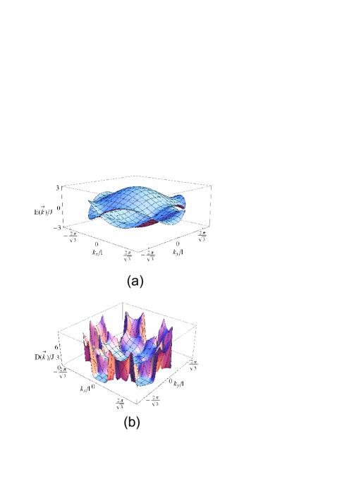
Figure 2: (a)The energy spectrum $E(k)$ of graphene versus $k$. (b)The interaction intensity $D(k)$ between electrons in graphene and single-mode light, in which we take the average over all the possible directions for e(q).

The single quasi-particle energy $E_{\mathbf{k}}$ and the interaction coefficient $D_{\mathbf{k,q}}$ are plotted versus the momentum $\mathbf{k}$ of the electrons in Fig. 2. The six Dirac points are clear to be found at the degeneracy points of upper and lower bands in Fig. 2(a). For the photon momentum $\left|\mathbf{q}\right|\mathbf{\ll\left|\mathbf{k}\right|}$ chosen in Fig. 2(b), the absolute value of the interaction coefficient $D_{\mathbf{k,q}}$ becomes large when $\mathbf{k}$ is near the boundary of the first Brillouin Zone and decreases rapidly as $\mathbf{k}$ deviate from that boundary.

III Interband Rabi Oscillation Induced by Strong Light Field

The general photon-electron interaction contains multi-mode light field, which case is too complex to be analytically treated in revealing the essential properties. Thus, we simplify the Hamiltonian by making the reasonable assumption that only one particular quantum mode of the light field would dominate the dynamics. This could be experimentally realized by adding a high-finesse microcavity to the system to pick out a single mode of quantized light under consideration. In this sense, the model Hamiltonian is reduced to $H=H_{0}+H_{1},$ where

$$H_{0} = \sum\limits_{\mathbf{k}}E_{\mathbf{k}}\left(\alpha_{\mathbf{k}}^{\dagger}\alpha_{\mathbf{k}}-\beta_{\mathbf{k}}^{\dagger}\beta_{\mathbf{k}}\right)+\Omega d^{\dagger}d,$$ (16a)

$$H_{1} = \sum_{\mathbf{k}}D_{\mathbf{k}}\left(d\alpha_{\mathbf{k}}^{\dagger}\beta_{\mathbf{k-q}}+h.c.\right),$$ (16b)

indicates that a single-mode light field would induce the coherent transitions of electrons between the upper band and the lower band. The output of the electronic flow would display an obvious resonance, namely, Rabi oscillation, which is experimentally observable.

In the strong light limit, the light field can be treated as a classical one, where the creation and annihilation operators $d^{\dagger}$ and $d$ are replaced by C-numbers, namely

$$d\rightarrow\sqrt{N}e^{-i\Omega t},d^{\dagger}\rightarrow\left(d\right)^{\ast}.$$ (17)

with $N$ the total number of photons. This approximation is valid since in a strong light field only the intensity of the light plays an important role. We can generally prove this classical approximation in App. A.

Then we obtain the semi-classical Hamiltonian $H(t)=\sum\limits_{\mathbf{k}}h_{\mathbf{k}}(t),$ in which the single momentum Hamiltonian is

$$h_{\mathbf{k}}(t) = E_{\mathbf{k}}\left(\alpha_{\mathbf{k}}^{\dagger}\alpha_{\mathbf{k}}-\beta_{\mathbf{k}-\mathbf{q}}^{\dagger}\beta_{\mathbf{k}-\mathbf{q}}\right)+$$ (18)

$$\sqrt{N}D_{\mathbf{k}}\left(\alpha_{\mathbf{k}}^{\dagger}\beta_{\mathbf{k}-\mathbf{q}}e^{-i\Omega t}+h.c.\right).$$

for electrons with momentum $\mathbf{k}$. Here, we have neglected the constant $N\Omega$ in the total energy of the light field and the difference between $E_{\mathbf{k}}$ and $E_{\mathbf{k-q}}$ for the reason mentioned at the end of Sec. II. In terms of the quasi-spin operators

$$S_{\mathbf{k}}^{z} = \frac{1}{2}\left(\alpha_{\mathbf{k}}^{\dagger}\alpha_{\mathbf{k}}-\beta_{\mathbf{k}-\mathbf{q}}^{\dagger}\beta_{\mathbf{k}-\mathbf{q}}\right),$$ (19a)

$$S_{\mathbf{k}}^{+} = \alpha_{\mathbf{k}}^{\dagger}\beta_{\mathbf{k}-\mathbf{q}},S_{\mathbf{k}}^{-}=\left(S_{\mathbf{k}}^{+}\right)^{\dagger},$$ (19b)

which obviously satisfy the commutation relations of the regular spin-$$1/2$$ operators, the above single momentum Hamiltonian is rewritten as

$$h_{\mathbf{k}}(t)=E_{\mathbf{k}}S_{\mathbf{k}}^{z}+\sqrt{N}D_{\mathbf{k}}\left(S_{\mathbf{k}}^{+}e^{-i\Omega t}+h.c.\right).$$ (20)

It describes a quasi-spin precession in a time-dependent effective magnetic field

$$\mathbf{B=(}\sqrt{N}D_{\mathbf{k}}\cos\Omega t,\sqrt{N}D_{\mathbf{k}}\sin\Omega t,E_{\mathbf{k}}\mathbf{).}$$ (21)

Such spin precession is just the Rabi oscillation between bands.

To solve the dynamic equation governed by $h_{\mathbf{k}}(t),$ a time-dependent unitary transformation

$$U(t)=\exp(i\Omega S_{\mathbf{k}}^{z}t),$$ (22)

is used to transform the Hamiltonian above into a time-independent one $h_{\mathbf{k}}^{\prime}=U^{\dagger}h_{\mathbf{k}}(t)U-i\partial_{t}U^{\dagger}U$ or

$$h_{\mathbf{k}}^{\prime}=-\Delta_{\mathbf{k}}S_{\mathbf{k}}^{z}+\sqrt{N}D_{\mathbf{k}}S_{\mathbf{k}}^{+}+h.c$$ (23)

Here,

$$\Delta_{\mathbf{k}}=\Omega-2E_{\mathbf{k}}.$$ (24)

is the detuning between the energy of the light field and that of the quasi-spin.

The Heisenberg equations of the system

$$i\frac{\partial}{\partial t}S_{\mathbf{k}}^{z} = \frac{1}{2}\varepsilon_{\mathbf{k}}\sin\theta_{\mathbf{k}}[S_{\mathbf{k}}^{+}-S_{\mathbf{k}}^{-}],$$ (25a)

$$i\frac{\partial}{\partial t}S_{\mathbf{k}}^{\pm} = \pm\varepsilon_{\mathbf{k}}[\cos\theta_{\mathbf{k}}S_{\mathbf{k}}^{\pm}+\sin\theta_{\mathbf{k}}S_{\mathbf{k}}^{z}],$$ (25b)

determine the Rabi oscillation of the electrons with momentum $$\mathbf{k} \theta_{\mathbf{k}}$$ between the upper and lower bands. Here the mixing angle is defined by

$$\cos\theta_{\mathbf{k}} = \frac{\Delta_{\mathbf{k}}}{\varepsilon_{\mathbf{k}}},$$ (26a)

$$\sin\theta_{\mathbf{k}} = \frac{2\sqrt{N}D_{\mathbf{k}}}{\varepsilon_{\mathbf{k}}},$$ (26b)

$$\varepsilon_{\mathbf{k}}^{2} = \Delta_{\mathbf{k}}^{2}+4ND_{\mathbf{k}}^{2}.$$ (26c)

The above first order partial differential equations (25a)-(25b) with initial operators $$S_{\mathbf{k}}^{z}(0) S_{\mathbf{k}}^{\pm}(0)$$ and is solved through the Laplace transformation

$$\lambda(p)=\int\limits_{0}^{+\infty}\lambda(t)e^{-pt}dt,$$ (27)

which gives

$$pS_{\mathbf{k}}^{z}-S_{\mathbf{k}}^{z}(0) = -i\frac{1}{2}\varepsilon_{\mathbf{k}}\sin\theta_{\mathbf{k}}[S_{\mathbf{k}}^{+}-S_{\mathbf{k}}^{-}],$$ (28a)

$$pS_{\mathbf{k}}^{\pm}-S_{\mathbf{k}}^{\pm}(0) = \mp i\varepsilon_{\mathbf{k}}[\cos\theta_{\mathbf{k}}S_{\mathbf{k}}^{\pm}+\sin\theta_{\mathbf{k}}S_{\mathbf{k}}^{z}].$$ (28b)

In terms of the normalized Laplacian parameter $$p^{\prime}=p/\varepsilon_{\mathbf{k}},$$ the above equation is solved as

$$S_{\mathbf{k}}^{z}(p^{\prime}) = \frac{S_{\mathbf{k}}^{z}(0)}{\varepsilon_{\mathbf{k}}}\frac{[p^{\prime 2}+\cos^{2}\theta_{\mathbf{k}}]}{p^{\prime}[p^{\prime 2}+1]}+\frac{S_{\mathbf{k}}^{y}(0)}{\varepsilon_{\mathbf{k}}}\frac{\sin\theta_{\mathbf{k}}}{p^{\prime 2}+1}$$ (29a)

$$-\frac{S_{\mathbf{k}}^{x}(0)}{\varepsilon_{\mathbf{k}}}\frac{\sin\theta_{\mathbf{k}}\cos\theta_{\mathbf{k}}}{p^{\prime}[p^{\prime 2}+1]},$$

$$S_{\mathbf{k}}^{\pm}(p^{\prime}) = \frac{1}{\varepsilon_{\mathbf{k}}}\frac{S_{\mathbf{k}}^{\pm}(0)\mp i\sin\theta_{\mathbf{k}}S_{\mathbf{k}}^{z}(p^{\prime})}{p^{\prime}\pm i\cos\theta_{\mathbf{k}}},$$ (29b)

where

$$S_{\mathbf{k}}^{x} = \frac{1}{2}(S_{\mathbf{k}}^{+}+S_{\mathbf{k}}^{-}),$$ (30a)

$$S_{\mathbf{k}}^{y} = \frac{1}{2i}(S_{\mathbf{k}}^{+}-S_{\mathbf{k}}^{-}).$$ (30b)

In the SWCNT, the electrons fill up the lower band when the system stays at its ground state at zero temperature. As a consequence, we may simply set $$S_{\mathbf{k}}^{x}(0) S_{\mathbf{k}}^{y}(0) S_{\mathbf{k}}^{z}(t) S_{\mathbf{k}}^{\pm}(t)$$ and as zero for convenience in the following discussions. The inverse Laplace transformation gives the time evolution of and respectively

$$S_{\mathbf{k}}^{z}(t)=S_{\mathbf{k}}^{z}(0)\left[\cos^{2}\theta_{\mathbf{k}}+\sin^{2}\theta_{\mathbf{k}}\cos\left(\varepsilon_{\mathbf{k}}t\right)\right].$$ (31)

and

$$S_{\mathbf{k}}^{\pm}(t) = -S_{\mathbf{k}}^{z}(0)\sin\theta_{\mathbf{k}}\cos\theta_{\mathbf{k}}[1-\cos\left(\varepsilon_{\mathbf{k}}t\right)]$$ (32)

$$\mp iS_{\mathbf{k}}^{z}(0)\sin\theta_{\mathbf{k}}\sin\left(\varepsilon_{\mathbf{k}}t\right).$$

Finally, the total population inversion

$$W(t)=\sum\limits_{\mathbf{k}}\left\langle S_{\mathbf{k}}^{z}(t)+\frac{1}{2}\right\rangle$$ (33)

is calculated as the summation over those of single momentum, which reads

$$W(t)=\sum\limits_{\mathbf{k}}\left\{\left\langle S_{\mathbf{k}}^{z}(0)\right\rangle\left[1-2\sin^{2}\theta_{\mathbf{k}}\sin^{2}\left(\frac{\varepsilon_{\mathbf{k}}t}{2}\right)\right]+\frac{1}{2}\right\}.$$ (34)

When the temperature is zero, the system stays at its ground state and thus $\left\langle S_{\mathbf{k}}^{z}(t=0)\right\rangle=-1/2$ is valid for all $\mathbf{k}$. Then the total population inversion is obtained

$$W(t)=\sum\limits_{\mathbf{k}}\frac{1}{2}\sin^{2}\theta_{\mathbf{k}}\{1-\cos\left(\varepsilon_{\mathbf{k}}t\right)\}$$ (35)

If we consider the continuous momentum in a 2-D graphene and the inhomogeneously-broadened system in which different quasi-spins have different momentums by introducing the distribution $g(\varepsilon_{\mathbf{k}})$ centered on $\varepsilon_{\mathbf{0}}$ as

$$g(\varepsilon_{\mathbf{k}})=2\sqrt{\pi}T\exp\left[-T^{2}\left(\varepsilon_{\mathbf{k}}-\varepsilon_{\mathbf{0}}\right)^{2}\right],$$ (36)

which satisfies $\frac{1}{2\pi}\int_{\infty}^{-\infty}g(\varepsilon_{\mathbf{k}})d\varepsilon_{\mathbf{k}}=1$. When $2\sqrt{N}D_{\mathbf{k}}\gg\Delta_{\mathbf{k}}$ results in $\sin\theta_{\mathbf{k}}\simeq 1$, the total population inversion can be calculated as

$$W(t) = \frac{1}{4\pi}\int_{\infty}^{-\infty}g(\varepsilon_{\mathbf{k}})\{1-\cos\left(\varepsilon_{\mathbf{k}}t\right)\}d\varepsilon_{\mathbf{k}}\mbox{}$$ (37)

$$= \frac{1}{2}\left[1-\cos\left(\varepsilon_{\mathbf{0}}t\right)\right]\exp\left(-\frac{t^{2}}{4T^{2}}\right).$$

It must be pointed out that the time dependence of the total population inversion includes two aspects when the energy distribution is Gaussian type. One is the periodic factor as $(1-\cos\left(\varepsilon_{\mathbf{0}}t\right))$ resulting from the central frequency of the Gaussian distribution. The other is the exponential decay $\exp\left(-\frac{t^{2}}{4T^{2}}\right)$ resulted from the broadening of the Gaussian distribution. The randomness of the energy spectrum of the quasi-spins actually induces these effects, which can be considered as a kind of spin echo.

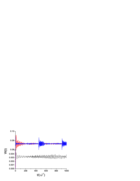
Figure 3: Population inversion of electrons in the SWCNT is plotted versus time. The parameters for the SWCNT are respectively: (1)chiral vector is $(6,4)$, $\Omega=0.4$, $\tau=5$ for the black short dotted line; (2)chiral vector is $(8,0)$, $\Omega=2$, $\tau=5$ for the red solid line; (3)chiral vector is $(8,0)$, $\Omega=2$, $\tau=70$ for the blue short dashed line. Here, $\tau$ is the time scale.

From Fig. 3 for the population inversion of the $(2n,0)$ SWCNTs with the incurring light frequency of $\Omega=2J$, we may see that a considerable proportion of the electrons are excited to the upper band (more than $1/15$ for $(8,0)$ SWCNT), and exhibits collapse and revival in a long period of time. The explanation for it is straightforward: in the $(2n,0)$ SWCNTs, there are large degeneracies of possible states onto the equi-energy lines $E=J$ of the $2$-D graphene energy bands. Thus, the $(2n,0)$ SWCNTs are potential experimental candidates for the demonstration of Rabi oscillation in solids.

IV First Order Coherence of Scattered and Emitted Photons

The strong light field only couples the upper and lower bands of electrons through its intensity, which essentially cancels the quantum optical features of the SWCNT characterized by the higher order quantum coherence. To save curiosity of quantized light field interacting with SWCNT, we return to the Hamiltonian Eq.(16a)-(16b)

The first order correlation function of the light field

$$G^{(1)}(\tau)=\left\langle d^{+}(t)d(t+\tau)\right\rangle$$ (38)

to characterize the interference of the electrons in SWCNT is independent of $t$ after long time evolution $t\rightarrow+\infty$, which corresponds to the steady solution for the light-SWCNT coupling system. In the interaction picture with respect to

$$H_{0}=\Omega d^{\dagger}d+\sum\limits_{\mathbf{k}}\Omega S_{\mathbf{k}}^{z},$$ (39)

the Langevin equations read as

$$\frac{\partial}{\partial t}d = -i\sum\limits_{\mathbf{k}}D_{\mathbf{k}}S_{\mathbf{k}}^{-},$$ (40a)

$$\frac{\partial}{\partial t}S_{\mathbf{k}}^{-} = \left(i\Delta_{\mathbf{k}}-\gamma_{\mathbf{k}}\right)S_{\mathbf{k}}^{-}+2iD_{\mathbf{k}}S_{\mathbf{k}}^{z}d,$$ (40b)

$$\frac{\partial}{\partial t}S_{\mathbf{k}}^{z} = -2\gamma_{\mathbf{k}}(S_{\mathbf{k}}^{z}+\frac{1}{2})+iD_{\mathbf{k}}(d^{\dagger}S_{\mathbf{k}}^{-}-S_{\mathbf{k}}^{+}d).$$ (40c)

Here, we phenomenologically add decay terms of the SWCNT part to the Langevin equations, while neglect the decay of light field since an ideal probe is considered. We also assume that the SWCNT system reaches its equilibrium state with the light field before there is considerable change in the light field. Actually, this assumption is very crucially used in Haken’s theory of laser Laser . By setting the time derivatives of the $$S$$ operators as zero, the steady solution of the total system can be obtained with steady quasi-spin operators

$$S_{\mathbf{k}}^{z} = -\frac{\gamma_{\mathbf{k}}^{2}+\Delta_{\mathbf{k}}^{2}}{2(\Delta_{\mathbf{k}}^{2}+2d^{\dagger}dD_{\mathbf{k}}^{2}+\gamma_{\mathbf{k}}^{2})},$$ (41a)

$$S_{\mathbf{k}}^{-} = -\frac{iD_{\mathbf{k}}(\gamma_{\mathbf{k}}-i\Delta_{\mathbf{k}})d}{\Delta_{\mathbf{k}}^{2}+2d^{\dagger}dD_{\mathbf{k}}^{2}+\gamma_{\mathbf{k}}^{2}}.$$ (41b)

Therefore, if the number of photons does not fluctuate intensively long time after the light is turned on, we could simply set the particle number operator $$d^{\dagger}d=N$$ as a constant.

In order to study the first order coherence of the light field, we use the mean field approach for the Langevin equations of the above system by setting

$$S_{\mathbf{k}}^{z}d\approx\left.\left\langle S_{\mathbf{k}}^{z}(t)\right\rangle\right|_{t\rightarrow\infty}d(\tau)\equiv S_{\mathbf{k}}^{z}(\infty)d(\tau)$$ (42)

for long time evolution. Here we can analytically calculate the first order correlation function through the partial differential equations (40a-40c). After applying Laplace transformation to Eq. (40a-40c), we have

$$pd-d(0) = -i\sum\limits_{\mathbf{k}}D_{\mathbf{k}}S_{\mathbf{k}}^{-},$$ (43a)

$$\left(p-i\Delta_{\mathbf{k}}^{\prime}\right)S_{\mathbf{k}}^{-} = 2iD_{\mathbf{k}}\left.\left\langle S_{\mathbf{k}}^{z}(t)\right\rangle\right|_{t\rightarrow\infty}d+S_{\mathbf{k}}^{-}(0),$$ (43b)

for the effective detuning $$\Delta_{\mathbf{k}}^{\prime}=\Delta_{\mathbf{k}}+i\gamma_{\mathbf{k}}. d(p)$$ This gives the solution of as

$$d(p)=\frac{d(0)+\Lambda^{-}(p)}{p-\Lambda^{z}(p)}.$$ (44)

Here,

$$\Lambda^{-}(p)=-i\sum\limits_{\mathbf{k}}\frac{D_{\mathbf{k}}S_{\mathbf{k}}^{-}(0)}{p-i\Delta_{\mathbf{k}}^{\prime}}$$ (45)

represents the contribution from $S_{\mathbf{k}}^{-}(0)$, while contribution from the long time evolution of $\left\langle S_{\mathbf{k}}^{z}\right\rangle$ is given by

$$\Lambda^{z}(p)=\sum\limits_{\mathbf{k}}\frac{2D_{\mathbf{k}}^{2}\left.\left\langle S_{\mathbf{k}}^{z}(t)\right\rangle\right|_{t\rightarrow\infty}}{p-i\Delta_{\mathbf{k}}^{\prime}}.$$ (46)

Since the electron-photon interaction serves as a perturbation term in the Hamiltonian, the singularities of the $d(p)$ is mainly determined by the denominator $p-\Lambda^{z}(p)$. Under the Wigner-Weisskopf approximation, the $0$-th order zero point of the denominator is $p=0,$ and to the $1$-st order it is

$$p=-i\Omega^{\prime}-\Gamma^{\prime},$$ (47)

where the renormalized frequency and the effective decay are

$$\Omega^{\prime} = -\mathrm{Im}\Lambda^{z}(0),$$ (48a)

$$\Gamma^{\prime} = -\mathrm{Re}\Lambda^{z}(0).$$ (48b)

Applying the inverse Laplace transformation, we obtain an expression for $$d(\tau)$$ as

$$d(\tau)=\exp\left(-i\Omega^{\prime}\tau-\Gamma^{\prime}\tau\right)\left[d(0)+F(\tau)\right],$$ (49)

where the contribution from $S_{\mathbf{k}}^{-}(0)$ is

$$F(\tau)=-i\sum\limits_{\mathbf{k}}\frac{D_{\mathbf{k}}S_{\mathbf{k}}^{-}(0)}{\mu_{\mathbf{k}}+i\nu_{\mathbf{k}}}\left[1-e^{-i\mu_{\mathbf{k}}\tau-\nu_{\mathbf{k}}\tau}\right],$$ (50)

with $\mu_{\mathbf{k}}=\left(-\Delta_{\mathbf{k}}-\Omega^{\prime}\right)$ and $\nu_{\mathbf{k}}=\left(\gamma_{\mathbf{k}}-\Gamma^{\prime}\right).$ If we compare a quasi-spin system to a heat bath, the term $F(\tau)$ represents its induced quantum fluctuation. The couplings of the light field to SWCNT is characterized by

$$\Omega^{\prime} = \sum\limits_{\mathbf{k}}\frac{D_{\mathbf{k}}^{2}}{\Delta_{\mathbf{k}}^{2}+2ND_{\mathbf{k}}^{2}+\gamma_{\mathbf{k}}^{2}}\Delta_{\mathbf{k}},$$ (51a)

$$\Gamma^{\prime} = \sum\limits_{\mathbf{k}}\frac{D_{\mathbf{k}}^{2}}{\Delta_{\mathbf{k}}^{2}+2ND_{\mathbf{k}}^{2}+\gamma_{\mathbf{k}}^{2}}\gamma_{\mathbf{k}},$$ (51b)

where the explicit steady solution for $$S_{\mathbf{k}}^{z}$$ that has been used.

The contribution $\left\langle d^{+}(0)F(\tau)\right\rangle$ from $S_{\mathbf{k}}^{-}(0)$ in the first order correlation

$$G^{(1)}(\tau)=\exp\left(-i\Omega^{\prime}\tau-\Gamma^{\prime}\tau\right)\left(G^{(1)}(0)+\left\langle d^{+}(0)F(\tau)\right\rangle\right)$$ (52)

vanishes since the average on the photon number states reduces to zero due to the photon number conservation. Then the normalized first order coherence function $g^{(1)}(\tau)\equiv G^{(1)}(\tau)/G^{(1)}(0)$ is explicitly written as

$$g^{(1)}(\tau)=\exp\left(-i\Omega^{\prime}\tau-\Gamma^{\prime}\tau\right),$$ (53)

which is used to measure the interference of the scattered and emitted photons. It is clear that long time first order correlation of the light field vanishes exponentially with $\tau$. In most cases, considering that the decay rates $\gamma_{\mathbf{k}}$ are much smaller than the detuning $\Delta_{\mathbf{k}}$, $\Gamma^{\prime}\ll\Omega^{\prime}$ is obviously satisfied. Thus, neglecting the decay effect in the first order coherence, the existence of SWCNT contributes to the first order coherence a shift $\Omega^{\prime}$ in the frequency of light.

V Second Order Correlation of The Scattered and Emitted Light

The first order coherence function only demonstrates the interference of the scattered and emitted photon. To distinguish the fully quantum optical properties of the SWCNT, e.g. , the bunching and anti-bunching of the photons, the second order coherence function

$$G^{(2)}(\tau)=\left\langle d^{\dagger}(t)d^{\dagger}(t+\tau)d(t+\tau)d(t)\right\rangle$$ (54)

is needed. According to Eq. (47), we calculate

$$G^{(2)}(\tau) = \exp\left(-2\Gamma^{\prime}\tau\right)G^{(2)}(0)$$ (55)

$$+\exp\left(-2\Gamma^{\prime}\tau\right)\left\langle d^{\dagger}(0)F^{\dagger}(\tau)F(\tau)d(0)\right\rangle,$$

where we have neglected terms $\left\langle d^{\dagger}(0)d^{\dagger}(0)F(\tau)d(0)\right\rangle$ and $\left\langle d^{\dagger}(0)F^{\dagger}(\tau)d(0)d(0)\right\rangle$ because of the photon number conservation for the light field. Neglecting correlation between different quasi-spins, only terms with the same momentum can survive in $F^{\dagger}(\tau)$ and $F(\tau).$ Therefore, the non-vanishing second term is calculated as

$$\left\langle d^{\dagger}(0)F^{\dagger}(\tau)F(\tau)d(0)\right\rangle$$ (56)

$$\approx \sum\limits_{\mathbf{k}}f_{\mathbf{k}}(\tau)\left\langle d^{\dagger}(0)S_{\mathbf{k}}^{+}(0)S_{\mathbf{k}}^{-}(0)d(0)\right\rangle$$

$$\approx \sum\limits_{\mathbf{k}}f_{\mathbf{k}}(\tau)\left\langle d^{\dagger}(0)d(0)\right\rangle\left(\left.\left\langle S_{\mathbf{k}}^{z}(t)\right\rangle\right|_{t\rightarrow\infty}+\frac{1}{2}\right),$$

where the time dependent coefficients are

$$f_{\mathbf{k}}(\tau)=\frac{2D_{\mathbf{k}}^{2}}{\mu_{\mathbf{k}}^{2}+\nu_{\mathbf{k}}^{2}}\left[\cosh\left(\nu_{\mathbf{k}}\tau\right)-\cos\left(\mu_{\mathbf{k}}\tau\right)\right]e^{-\nu_{\mathbf{k}}\tau}.$$ (57)

Accordingly, the normalized second order coherence function $g^{(2)}(\tau)\equiv G^{(2)}(\tau)/\left|G^{(1)}(0)\right|^{2}$ is written as

$$g^{(2)}(\tau) = \exp\left(-2\Gamma^{\prime}\tau\right)\left[\frac{G^{(2)}(0)}{G^{(1)}(0)^{2}}\right.+$$ (58)

$$\left.\sum\limits_{\mathbf{k}}\frac{f_{\mathbf{k}}(\tau)}{G^{(1)}(0)}\left(\left.\left\langle S_{\mathbf{k}}^{z}(t)\right\rangle\right|_{t\rightarrow\infty}+\frac{1}{2}\right)\right]$$

Here, the second item in $g^{(2)}(\tau)$ is non-negative for any $\tau$, and returns to zero when $\tau\rightarrow 0$, thus  the explicit effect of the anti-bunching of the light coupled with the SWCNT is illustrated in Fig.  4.

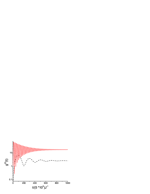
Figure 4: The second order correlation of the light $g^{(2)}(t)-g^{(2)}(0)$ is plotted, in which the antibunching feature is obviously displayed. The two chiral vectors $(6,4)$ and $(8,0)$ are chosen to represent significant anti-bunching effect due to different reasons. Here, we have chosen the frequency of the light field $\omega=2J$.

Due to the divergence near the resonance area for $g^{(2)}(t)$, the anti-bunching feature is significant where the light and the energy gap between upper and lower bands reach resonance while the interaction intensity $D_{\mathbf{k}}$ is comparatively high. In this case, the SWCNT is equivalent to one or several 2-level atoms that interact strongly with the incurring light, just as the case in the $(6,4)$ SWCNT when the incurring light frequency is $2J$. Similar to Sec. III concerning Rabi oscillation, here we still have a distinct effect for the $(2n,0)$ SWCNTs, when the incurring light frequency is really close to $2J$. In the case for $(8,0)$ SWCNT, the strong anti-bunching feature is instead caused by the large degeneracy on the $E=J$ line in the first Brillouin zone. Unlike the case for the $(6,4)$ SWCNT, in which merely several electron states are involved, the significant anti-bunching here is caused by the excitation in the $E=J$ band of the SWCNT, where thousands of possible states participate in at the same time.

VI Possible Lasing Mechanism of Carbon Nanotube

The above investigations imply that the light emitted from or scattered by the SWCNT is strongly correlated in time domain, thus explicitly displays quantum effects. It is straight forward to imagine that if electrons in the SWCNT experience a population inversion, the emitted light would be amplified. This observation may enable a possible lasing mechanism. In this section, we will explore this mechanism for the SWCNT by using Haken’s laser theory  Laser .

The Heisenberg equations(25a,25b) without dissipation usually have no steady solution. Thus we phenomenologically introduce decays on both the light field and the quasi-spin operators to make the physical observables reach the stable results. In order to obtain the steady solution, we neglect the fluctuations because the time average of them vanishes. This simplification results in the laser-like equations

$$\frac{\partial}{\partial t}\widetilde{d}^{\dagger} = -\kappa\widetilde{d}^{\dagger}+i\sum\limits_{\mathbf{k}}D_{\mathbf{k}}\widetilde{S}_{\mathbf{k}}^{+}e^{-i\Delta_{\mathbf{k}}t},$$ (59a)

$$\frac{\partial}{\partial t}\widetilde{S}_{\mathbf{k}}^{+} = -\gamma_{\mathbf{k}}\widetilde{S}_{\mathbf{k}}^{+}-2iD_{\mathbf{k}}\widetilde{d}^{\dagger}S_{\mathbf{k}}^{z}e^{i\Delta_{\mathbf{k}}t},$$ (59b)

$$\frac{\partial}{\partial t}S_{\mathbf{k}}^{z} = -2\gamma_{\mathbf{k}}(S_{\mathbf{k}}^{z}+\frac{1}{2})-iD_{\mathbf{k}}(\widetilde{S}_{\mathbf{k}}^{+}\widetilde{d}e^{-i\Delta_{\mathbf{k}}t}-h.c.),$$ (59c)

where we have removed the higher frequency factors by defining $\widetilde{d}^{\dagger}=d^{\dagger}\exp(-i\Omega t)$ and $\widetilde{S}_{\mathbf{k}}^{+}=S_{\mathbf{k}}^{+}\exp[-i2E(\overrightarrow{k})t].$ This approach changes the observation from a laboratory frame of reference into some rotating one. Equation (59b) can be formally integrated as

$$\widetilde{S}_{\mathbf{k}}^{+}(t)=\widetilde{S}_{\mathbf{k}}^{+}(0)e^{-\gamma_{\mathbf{k}}t}-2iD_{\mathbf{k}}\int\limits_{0}^{t}e^{-\gamma_{\mathbf{k}}(t-\tau)}\widetilde{d}^{\dagger}S_{\mathbf{k}}^{z}e^{i\Delta_{\mathbf{k}}\tau}d\tau.$$ (60)

According to Haken’s laser theory, if $\widetilde{d}^{\dagger}S_{\mathbf{k}}^{z}$ varies with time much slower than $\widetilde{S}_{\mathbf{k}}^{+}(t)$, it could be regarded as a time-independent one and then the above integral becomes

$$\widetilde{S}_{\mathbf{k}}^{+}(t)=\widetilde{S}_{\mathbf{k}}^{+}(0)e^{-\gamma_{\mathbf{k}}t}-2iD_{\mathbf{k}}\widetilde{d}^{\dagger}S_{\mathbf{k}}^{z}\frac{\left(e^{i\Delta_{\mathbf{k}}t}-e^{-\gamma_{\mathbf{k}}t}\right)}{\gamma_{\mathbf{k}}+i\Delta_{\mathbf{k}}},$$ (61)

After a long time, the first term in the above solution Eq.(60), which is totally determined by the initial polarization $\widetilde{S}_{\mathbf{k}}^{+}(0)$, will vanish. Thus, when $\gamma_{k}t\gg 1$, only the initial state-independent part

$$\widetilde{S}_{\mathbf{k}}^{+}(t)\approx-2iD_{\mathbf{k}}\widetilde{d}^{\dagger}S_{\mathbf{k}}^{z}\frac{e^{i\Delta_{\mathbf{k}}t}}{\gamma_{\mathbf{k}}+i\Delta_{\mathbf{k}}},$$ (62)

remains. In this case the motion equation of the $z-$direction spin operators becomes

$$\frac{\partial}{\partial t}S_{\mathbf{k}}^{z}\approx-2\gamma_{\mathbf{k}}(S_{\mathbf{k}}^{z}+\frac{1}{2})-\theta_{\mathbf{k}}\widetilde{d}^{\dagger}\widetilde{d}S_{\mathbf{k}}^{z},$$ (63)

where $\theta_{\mathbf{k}}=4\gamma_{\mathbf{k}}D_{\mathbf{k}}^{2}/(\gamma_{\mathbf{k}}^{2}+\Delta_{\mathbf{k}}^{2})$. Then we obtain the effective motion equation of the light field

$$\frac{\partial}{\partial t}\widetilde{d}^{\dagger}=-\widetilde{d}^{\dagger}\left(\kappa-\sum\limits_{\mathbf{k}}\frac{2D_{\mathbf{k}}^{2}e^{i\Omega t}}{\gamma_{\mathbf{k}}+i\Delta_{\mathbf{k}}}S_{\mathbf{k}}^{z}\right).$$ (64)

In the following discussions we will demonstrate a lasing-like phenomenon by considering the solution of Eq.(64)

Usually, a lasing process requires population inversion. To realize such population inversion in our setup, a pump of electrons is needed to inject electrons with specific state into the carbon nanotube. Phenomenologically, we add a pump term $c_{\mathbf{k}}>0$ to each term $S_{\mathbf{k}}^{z}$, then

$$\frac{\partial}{\partial t}S_{\mathbf{k}}^{z}=c_{\mathbf{k}}-2\gamma_{\mathbf{k}}(S_{\mathbf{k}}^{z}+\frac{1}{2})-\theta(\mathbf{k})\widetilde{d}^{\dagger}\widetilde{d}S_{\mathbf{k}}^{z},$$ (65)

The population inversion is obtained from Eq. (65) as

$$S_{\mathbf{k}}^{z} = S_{\mathbf{k}}^{z}(0)\exp\left(-\int\limits_{0}^{t}\left[\theta_{\mathbf{k}}\widetilde{d}^{\dagger}\widetilde{d}+2\gamma_{\mathbf{k}}\right]d\tau^{\prime}\right)+$$ (66)

$$(c_{\mathbf{k}}-\gamma_{\mathbf{k}})\int\limits_{0}^{t}\exp\left(\int\limits_{0}^{\tau}\left[\theta_{\mathbf{k}}\widetilde{d}^{\dagger}\widetilde{d}+2\gamma_{\mathbf{k}}\right]d\tau^{\prime}\right)d\tau\times$$

$$\exp\left(-\int\limits_{0}^{t}\left[\theta_{\mathbf{k}}\widetilde{d}^{\dagger}\widetilde{d}+2\gamma_{\mathbf{k}}\right]d\tau^{\prime}\right).$$

After a long time evolution $\left(\gamma_{\mathbf{k}}t\gg 1\right)$, this solution becomes

$$S_{\mathbf{k}}^{z}=(c_{\mathbf{k}}-\gamma_{\mathbf{k}})\int\limits_{0}^{t}\exp\left(-\int\limits_{\tau}^{t}\theta_{\mathbf{k}}\widetilde{d}^{\dagger}\widetilde{d}d\tau^{\prime}\right)e^{-2\gamma_{\mathbf{k}}(t-\tau)}d\tau.$$ (67)

It follows from Eq.(67) that the main contribution of the integral comes from the accumulation of the weighted photon numbers in the time $\tau\sim t$. In this sense we can assume that

$$\int\limits_{\tau}^{t}\theta_{\mathbf{k}}\widetilde{d^{\dagger}}\widetilde{d}d\tau^{\prime}=\theta_{\mathbf{k}}\widetilde{d^{\dagger}}\widetilde{d}(t-\tau)$$

Then the population inversion is integrated as

$$S_{\mathbf{k}}^{z}\approx\frac{(c_{\mathbf{k}}-\gamma_{\mathbf{k}})}{\theta_{\mathbf{k}}\widetilde{d}^{\dagger}\widetilde{d}+2\gamma_{\mathbf{k}}}.$$ (68)

Eventually, the motion equation of the light field is obtained as

$$\frac{\partial}{\partial t}\widetilde{d}^{\dagger}\approx(\kappa^{\prime}-i\delta\omega)\widetilde{d}^{\dagger}-\eta\widetilde{d}^{\dagger}\widetilde{d}^{\dagger}\widetilde{d},$$ (69)

where

$$\delta\omega=\sum\limits_{\mathbf{k}}D_{\mathbf{k}}^{2}\frac{(c_{\mathbf{k}}-\gamma_{\mathbf{k}})}{\gamma_{\mathbf{k}}}\frac{\Delta_{\mathbf{k}}}{\gamma_{\mathbf{k}}^{2}+\Delta_{\mathbf{k}}^{2}},$$ (70a)

appears as the Lamb shift of photons, and

$$\kappa^{\prime}=-\kappa+\sum\limits_{\mathbf{k}}D_{\mathbf{k}}^{2}\frac{(c_{\mathbf{k}}-\gamma_{\mathbf{k}})}{\gamma_{\mathbf{k}}^{2}+\Delta_{\mathbf{k}}^{2}},$$ (70b)

represents a dissipation or amplification of the optical mode together with

$$\eta=\sum\limits_{\mathbf{k}}2D_{\mathbf{k}}^{4}\frac{c_{\mathbf{k}}-\gamma_{\mathbf{k}}}{(\gamma_{\mathbf{k}}^{2}+\Delta_{\mathbf{k}}^{2})^{2}}.$$ (70c)

describing the extent of nonlinearity of the light field induced by the SWCNT. Here, we have expanded the second item on the right hand side of Eq.(69) up to the first order of $$2D_{\mathbf{k}}^{2}\widetilde{d}^{\dagger}\widetilde{d}$$.

Obviously, Eq.(69) is typical to describe the lasing process in an amplification medium. When electrons are injected into the SWCNT to realize a population inversion,

$$\kappa^{\prime}=-\kappa+\sum\limits_{\mathbf{k}}D_{\mathbf{k}}^{2}\frac{(c_{\mathbf{k}}-\gamma_{\mathbf{k}})}{\gamma_{\mathbf{k}}^{2}+\Delta_{\mathbf{k}}^{2}}>0$$ (71)

with $\eta>0$, we obtain a lasing equation

$$\frac{\partial}{\partial t}\widetilde{d^{\dagger}}=\kappa^{\prime}\widetilde{d^{\dagger}}-\eta\widetilde{d^{\dagger}}\widetilde{d^{\dagger}}\widetilde{d}.$$ (72)

Then the effect of the coherently injected electrons the SWCNT on the light field is equivalent to that of a double-well potential formed as

$$V(\left|d\right|)=-\kappa^{\prime}\left|d\right|^{2}+\frac{\eta}{2}\left|d\right|^{4},$$ (73)

Thus there exists a symmetry breaking based instability for laser amplification. When $\kappa^{\prime}<0$, $d=0$ is the unique stable point for the effective potential $V(\left|d\right|)$. In this case we may safely neglect the nonlinearity, and the system is only affected by stochastic processes. However, when $\kappa^{\prime}$ passes through zero, the point $d=0$ is no longer the stable point. Instead, the photon amplitude $d$ acquires its new stable points with nonzero amplitude

$$\left|d\right|=\sqrt{\frac{\kappa^{\prime}}{\eta}}$$ (74)

indicating a phase transition in the system. The above phenomenon that nonzero stable points of $V(\left|d\right|)$appear means that a coherent light field with non-vanishing amplitude is produced by the radiation of electrons confined in the SWCNT.

VII Conclusion

In summary, our investigation in this paper is oriented by the needs of designing the quantum devices in future. We theoretically studied a solid state based quantum optical system, namely, the SWCNT interacting with quantized light field. The ballistic transport of electrons in SWCNT means quantum coherence of electrons in terminology of quantum optics. Thus, the emitted and scattered light from such coherent electrons could be quantum coherent as well, and then we use the higher order coherence function to describe it. On the other hand, SWCNT with different chirality $(n,m)$ have different properties in their Rabi oscillations of the electrons when driven by a strong single-mode light field. The anti-bunching features of the light scattered by or emitted from them is also studied in details here. The reason for such distinction of chirality is that different sets of wave vectors $\mathbf{k}$ are allowed in SWCNT with different chiral vectors, which may lead to different energy structures in the SWCNT. Such effect is especially significant on the $(2n,0)$ type SWCNT, where large degeneracy of possible electron states onto $E=J$ occurs. This is a characteristic property absent in 2D graphene. The possible lasing mechanism in the SWCNT is also investigated theoretically, which may promise the realization of nanoscale laser devices.

Appendix A Semi-classical

It is noticed that the semi-classical approximation applied in Sec. III is valid only for the quasi-classical case in which the initial state possesses a very large number of single frequency photons. We will justify this approximation with necessary details in this appendix.

The complete dynamics of the SWCNT interacting with a strong light field is displayed through the Schrodinger equations governed by the Hamiltonian $H=H_{0}+H_{1},$ in the interaction picture, where

$$H_{0} = \sum\limits_{\mathbf{k}}E_{\mathbf{k}}\left(\alpha_{\mathbf{k}}^{\dagger}\alpha_{\mathbf{k}}-\beta_{\mathbf{k}}^{\dagger}\beta_{\mathbf{k}}\right),$$ (75a)

$$H_{1} = \sum_{\mathbf{k}}D_{\mathbf{k}}\left(de^{-i\Omega t}\alpha_{\mathbf{k}}^{\dagger}\beta_{\mathbf{k-q}}+h.c.\right)$$ (75b)

And the initial condition of the system

$$\left|\Psi\left(0\right)\right\rangle=\left|\xi=\sqrt{N}e^{i\theta}\right\rangle\otimes\left|\phi\left(0\right)\right\rangle,$$ (76)

where the coherent state

$$\left|\xi\right\rangle=\exp\left(\xi d^{\dagger}-\xi^{\ast}d\right)\left|0\right\rangle\equiv D\left(\xi\right)\left|0\right\rangle$$ (77)

represents the state of the light field while $\left|\phi\left(0\right)\right\rangle$ stands for the initial state of the electrons in the SWCNT. We note that $\left|\alpha\right|\simeq\sqrt{N}.$Since there is no broken global phase symmetry, the arbitrary $\theta$ is chosen as $0.$ The main reason for choosing the initial photon state as a coherent one is that the average number $\left\langle\sqrt{N}\right|d^{\dagger}d\left|\sqrt{N}\right\rangle=N$ should be satisfied.

We introduce the photon vacuum picture, similar to the approach for the semi-classical approximation of photon-atom system [cite P.L.Kingt Concept of Quantum Optics], defined by

$$\left|\Phi\left(t\right)\right\rangle=D\left(\xi\right)^{-1}\left|\Psi\left(t\right)\right\rangle,\left|\Phi\left(0\right)\right\rangle=\left|0\right\rangle\otimes\left|\phi\left(0\right)\right\rangle$$ (78)

which satisfies the Schrodinger equation (in the interaction picture) with the effective Hamiltonian

$$H_{e}=D\left(\xi\right)^{-1}HD\left(\xi\right)=H_{0}+V_{q}+H_{q}$$

where

$$V_{q} = \sum_{\mathbf{k}}D_{\mathbf{k}}\left(\sqrt{N}e^{-i\Omega t}\alpha_{\mathbf{k}}^{\dagger}\beta_{\mathbf{k-q}}+h.c.\right)$$ (79a)

$$H_{q} = \sum_{\mathbf{k}}D_{\mathbf{k}}\left(de^{-i\Omega t}\alpha_{\mathbf{k}}^{\dagger}\beta_{\mathbf{k-q}}+h.c.\right),$$ (79b)

Here $|0\rangle$ can be understood as a displaced vacuum. It should be noticed that the above derivation is exact for the initial condition (78).

For a very large $N$, $H_{q}$ in the above Hamiltonian is very small with respect to the $V_{q}$, and it can be neglected in the first order approximation. Under this approximation, the state of photons is subjected to a collective evolution governed by the effective Hamiltonian

$$H_{e} = H_{0}+V_{q},$$ (80a)

$$V_{q} = \sum_{\mathbf{k}}D_{\mathbf{k}}\left(\sqrt{N}e^{-i\Omega t}\alpha_{\mathbf{k}}^{\dagger}\beta_{\mathbf{k-q}}+h.c.\right).$$ (80b)

Transforming back to the original picture, one proves the conclusion: If $$N |\Psi(t)\rangle=|\sqrt{N}e^{i\theta}\rangle\otimes|\phi(t)\rangle, |\phi(t)\rangle H_{e}$$ is a macroscopic number, namely, it is large enough, the total system will evolve with a factorizable wave function where obeys the Schrödinger equation governed by the effective Hamiltonian .

The next question is the effects of the neglected term, $H_{q}$, on the dynamics in the photons vacuum picture. In the framework of the perturbation theory, the role of $H_{q}$ relies on the coupling to the vacuum, that is

$$H_{q}|\Phi(0)\rangle = \sum_{\mathbf{k}}D_{\mathbf{k}}\left(de^{-i\Omega t}\alpha_{\mathbf{k}}^{\dagger}\beta_{\mathbf{k-q}}+h.c.\right)|0\rangle\otimes|\phi(0)\rangle$$ (81)

$$= e^{i\Omega t}|1\rangle\otimes\sum_{\mathbf{k}}D_{\mathbf{k}}\beta_{\mathbf{k-q}}^{\dagger}\alpha_{\mathbf{k}}|\phi(0)\rangle$$

which leads to a single-particle excitation of the vacuum. Finally we reach the following conclusions: (1) In the large $N$ limit, this excitation is weak compared with the collective motion; (2) If there is initially no collective excitation or single excited electrons in the SWCNT, the system will be stable and remain in the displaced vacuum state even when $H_{q}$ is taken into account.

References

• (1) R. Saito, G. Dresselhaus, M. S. Dresselhaus, Physical Properties of Carbon Nanotubes (Imperial College Press, London, 1995).
• (2) R. H. Baughman, A. A. Zakhidov, W. A. de Heer, Science 297, 787 (2002).
• (3) M. S. Dresselhaus, G. Dresselhaus, Ph. Avouris, Carbon Nanotubes (Springer-Verlag, Berlin, 2110).
• (4) M. J. O’Connell, S. M. Bachilo, C. B. Huffman, V. C. Moore, M. S. Strano, E. H. Haroz, K. L. Rialon, P. J. Boul, W. H. Noon, C. Kittrell, Jianpeng Ma, R. H. Hauge, R. Bruce Weisman, and R. E. Smalley, Science 297, 593 (2002).
• (5) V. C. Moore, M. S. Strano, E. H. Haroz, R. H. Hauge, and R. E. Smalley, Nano Lett. 3, 1379 (2003).
• (6) Chongwu Zhou, Jing Kong, and Hongjie Dai, Appl. Phys. Lett. 76, 1597 (2000).
• (7) M. Y. Sfeir, T. Beetz, F. Wang, Limin Huang, X. M. H. Huang, Mingyuan Huang, J. Hone, S. O’Brien, J. A. Misewich, T. F. Heinz, Lijun Wu, Yimei Zhu, and L. E. Brus, Science 312, 554 (2006).
• (8) A. Javey, J. Guo, Q. Wang, M. Lundstrom, and Hongjie Dai, Nature 424, 654 (2003).
• (9) Xiaolei Liu, Chenglung Lee, and Chongwu Zhou, Appl. Phys. Lett. 79, 3329 (2001).
• (10) Z. Y. Zhang, S. Wang, L. Ding, X. L. Liang, H. L. Xu, J. Shen, Q. Chen, R. L. Cui, Y. Li, and L. M. Peng, Appl. Phys. Lett. 92, 133117 (2008).
• (11) S. M. Bachilo, M. S. Strano, C. Kittrell, R. H. Hauge, R. E. Smalley, R. B. Weisman, Science 298, 2361 (2002).
• (12) H. Katauraa, Y. Kumazawaa, Y. Maniwaa, I. Umezub, S. Suzukic, Y. Ohtsukac and Y. Achiba, Synthetic Metals 103, 2555 (1999).
• (13) E. Chang, G. Bussi, A. Ruini, and E. Molinari, Phys. Rev. Lett. 92, 196401 (2004).
• (14) C. D. Spataru, S. Ismail-Beigi, L. X. Benedict, and S. G. Louie, Phys. Rev. Lett. 92, 077402 (2004).
• (15) V. Perebeinos, J. Tersoff, and Ph. Avouris, Phys. Rev. Lett. 92, 257402 (2004).
• (16) H. Zhao and S. Mazumdar, Phys. Rev. Lett. 93, 157402 (2004).
• (17) F. Wang, G. Dukovic, L. E. Brus, T. F. Heinz, Science 308, 838 (2005).
• (18) J. Maultzsch, R. Pomraenke, S. Reich, E. Chang, D. Prezzi, A. Ruini, E. Molinari, M. S. Strano, C. Thomsen, and C. Lienau, Phys. Rev. B 72, 241402 (2005).
• (19) J. Lefebvre and P. Finnie, Phys. Rev. Lett. 98, 167406 (2007).
• (20) A.Höele, C. Galland, M. Winger, and A. Imamoǧlu, Phys. Rev. Lett. 100, 217401 (2008).
• (21) H. Haken, Rev. Mod. Phys. 47, 67 (1975).