Root polytopes, triangulations, and the subdivision algebra, I

Abstract.

The type $A_{n}$ root polytope $\mathcal{P}(A_{n}^{+})$ is the convex hull in $\mathbb{R}^{n+1}$ of the origin and the points $e_{i}-e_{j}$ for $1\leq i<j\leq n+1$. Given a tree $T$ on the vertex set $[n+1]$, the associated root polytope $\mathcal{P}(T)$ is the intersection of $\mathcal{P}(A_{n}^{+})$ with the cone generated by the vectors $e_{i}-e_{j}$, where $(i,j)\in E(T)$, $i<j$. The reduced forms of a certain monomial $m[T]$ in commuting variables $x_{ij}$ under the reduction $x_{ij}x_{jk}\rightarrow x_{ik}x_{ij}+x_{jk}x_{ik}+\beta x_{ik}$, can be interpreted as triangulations of $\mathcal{P}(T)$. Using these triangulations, the volume and Ehrhart polynomial of $\mathcal{P}(T)$ are obtained. If we allow variables $x_{ij}$ and $x_{kl}$ to commute only when $i,j,k,l$ are distinct, then the reduced form of $m[T]$ is unique and yields a canonical triangulation of $\mathcal{P}(T)$ in which each simplex corresponds to a noncrossing alternating forest. Most generally, the reduced forms of all monomials in the noncommutative case are unique.

1. Introduction

In this paper we develop the connection between triangulations of type $A_{n}$ root polytopes and two closely related algebras: the subdivision algebra $\mathcal{S}(A_{n})$ and the algebra $\mathcal{B}(A_{n})$, which we call the quasi-classical Yang-Baxter algebra following A. N. Kirillov. The close connection of the root polytopes and the algebras $\mathcal{S}(A_{n})$ and $\mathcal{B}(A_{n})$ is displayed by the variety of results this connection yields: both in the realm of polytopes and in the realm of the algebras. Two closely related algebras with tight connections to Schubert calculus have been studied by Fomin and Kirillov in [FK] and by Kirillov in [K1]. Before stating definitions and reasons, we pause at Exercise 6.C6 of Stanley’s Catalan Addendum [S1] to learn the following.

Consider the monomial $w=x_{12}x_{23}\cdots x_{n,n+1}$ in commuting variables $x_{ij}$. Starting with $p_{0}=w$, produce a sequence of polynomials $p_{0},p_{1},\ldots,p_{m}$ as follows. To obtain $p_{r+1}$ from $p_{r}$, choose a term of $p_{r}$ which is divisible by $x_{ij}x_{jk}$, for some $i,j,k$, and replace the factor $x_{ij}x_{jk}$ in this term with $x_{ik}(x_{ij}+x_{jk})$. Note that $p_{r+1}$ has one more term than $p_{r}$. Continue this process until a polynomial $p_{m}$ is obtained, in which no term is divisible by $x_{ij}x_{jk}$, for any $i,j,k$. Such a polynomial $p_{m}$ is a reduced form of $w$. Exercise 6.C6 in [S1] states that, remarkably, while the reduced form is not unique, it turns out that the number of terms in a reduced form is always the Catalan number $C_{n}=\frac{1}{n+1}{2n\choose n}$.

The angle from which we look at this problem gives a perspective reaching far beyond its setting in the world of polynomials. On one hand, the reductions can be interpreted in terms of root polytopes and their subdivisions, yielding a geometric, and subsequently a combinatorial, interpretation of reduced forms. On the other hand, using the combinatorial results obtained about the reduced forms, we obtain a method for calculating the volumes and Ehrhart polynomials of a family of root polytopes.

Root polytopes were defined by Postnikov in [P]. The full root polytope $\mathcal{P}(A_{n}^{+})$, which is the convex hull in $\mathbb{R}^{n+1}$ of the origin and points $e_{i}-e_{j}$ for $1\leq i<j\leq n+1$, already made an appearance in the work of Gelfand, Graev and Postnikov [GGP], who gave a canonical triangulation of it in terms of noncrossing alternating trees on $[n+1]$. We obtain canonical triangulations for all acyclic root polytopes, of which $\mathcal{P}(A_{n}^{+})$ is a special case.

We define acyclic root polytopes $\mathcal{P}(T)$ for a tree $T$ on the vertex set $[n+1]$ as the intersection of $\mathcal{P}(A_{n}^{+})$ with a cone generated by the vectors $e_{i}-e_{j}$, where $(i,j)\in E(T)$, $i<j$. Let

$$\overline{G}=([n+1],\{(i,j)\mid\mbox{there exist edges $(i,i_{1})\ldots,(i_{k},j)$ in $G$ such that}$$

$i<i_{1}<\ldots<i_{k}<j\}),$

denote the transitive closure of the graph $G$. Recall that a graph $G$ on the vertex set $[n+1]$ is said to be noncrossing if there are no vertices $i<j<k<l$ such that $(i,k)$ and $(j,l)$ are edges in $G$. A graph $G$ on the vertex set $[n+1]$ is said to be alternating if there are no vertices $i<j<k$ such that $(i,j)$ and $(j,k)$ are edges in $G$. Alternating trees were introduced in [GGP]. Gelfand, Graev and Postnikov [GGP] showed that the number of noncrossing alternating trees on $[n+1]$ is counted by the Catalan number $C_{n}$.

Theorem 1.

If $T$ is a noncrossing tree on the vertex set $[n+1]$ and $T_{1},\ldots,T_{k}$ are the noncrossing alternating spanning trees of $\overline{T}$, then the root polytopes $\mathcal{P}(T_{1}),\ldots,\mathcal{P}(T_{k})$ are $n$-dimensional simplices with disjoint interiors whose union is $\mathcal{P}(T)$. Furthermore,

$$\mbox{\em vol}\,\mathcal{P}(T)=f_{T}\frac{1}{n!},$$

where $f_{T}$ denotes the number of noncrossing alternating spanning trees of $\overline{T}$.

Theorem 1 can be generalized in a few directions. We calculate the Ehrhart polynomial of $\mathcal{P}(T)$; see Sections 5 and 8. We describe the intersections of the top dimensional simplices $\mathcal{P}(T_{1}),\ldots,\mathcal{P}(T_{k})$ in Theorem 1 in terms of noncrossing alternating spanning forests of $\overline{T}$ in Section 8. Theorem 1 and its generalizations can also be proved for any forest $F$, not necessarily noncrossing, as explained in Section 9. In Section 9 we also prove that the triangulation in Theorem 1 is shellable, and provide a second method for calculating the Ehrhart polynomial of $\mathcal{P}(T)$.

The proof of Theorem 1 relies on relating the triangulations of a root polytope $\mathcal{P}(T)$ to reduced forms of a monomial $m[T]$ in variables $x_{ij}$, which we now define. Let $\mathcal{S}(A_{n})$ and $\mathcal{B}(A_{n})$ be two associative algebras over the polynomial ring $\mathbb{Q}[\beta]$, where $\beta$ is a variable (and a central element), generated by the set of elements $\{x_{ij}\mid 1\leq i<j\leq n+1\}$ modulo the relation $x_{ij}x_{jk}=x_{ik}x_{ij}+x_{jk}x_{ik}+\beta x_{ik}$. The subdivision algebra $\mathcal{S}(A_{n})$ is commutative, i.e., it has additional relations $x_{ij}x_{kl}=x_{kl}x_{ij}$ for all $i,j,k,l$, while $\mathcal{B}(A_{n})$, which we call the quasi-classical Yang-Baxter algebra following Kirillov [K2], is noncommutative and has additional relations $x_{ij}x_{kl}=x_{kl}x_{ij}$ for $i,j,k,l$ distinct only. The motivation for calling $\mathcal{S}(A_{n})$ the subdivision algebra is simple; the relations of $\mathcal{S}(A_{n})$ yield certain subdivisions of root polytopes, which we explicitly demonstrate by the Reduction Lemma (Lemma 5).

We treat the first relation as a reduction rule:

(1) $$x_{ij}x_{jk}\rightarrow x_{ik}x_{ij}+x_{jk}x_{ik}+\beta x_{ik}.$$

A reduced form of the monomial $m$ in the algebra $\mathcal{S}(A_{n})$ (algebra $\mathcal{B}(A_{n})$) is a polynomial $P_{n}^{\mathcal{S}}$ (polynomial $P_{n}^{\mathcal{B}}$) obtained by successive applications of reduction (1) until no further reduction is possible, where we allow commuting any two variables (commuting any two variables $x_{ij}$ and $x_{kl}$ where $i,j,k,l$ are distinct) between reductions. Note that the reduced forms are not necessarily unique.

A possible sequence of reductions in algebra $\mathcal{S}(A_{n})$ yielding a reduced form of $x_{12}x_{23}x_{34}$ is given by

(2) $$x_{12}\mbox{\boldmath$x_{23}x_{34}$} \rightarrow \mbox{\boldmath$x_{12}$}x_{24}\mbox{\boldmath$x_{23}$}+\mbox{\boldmath$x_{12}$}x_{34}\mbox{\boldmath$x_{24}$}+\beta\mbox{\boldmath$x_{12}x_{24}$}$$

$$\rightarrow \mbox{\boldmath$x_{24}$}x_{13}\mbox{\boldmath$x_{12}$}+x_{24}x_{23}x_{13}+\beta x_{24}x_{13}+x_{34}x_{14}x_{12}+x_{34}x_{24}x_{14}$$

$$+\beta x_{34}x_{14}+\beta x_{14}x_{12}+\beta x_{24}x_{14}+\beta^{2}x_{14}$$

$$\rightarrow x_{13}x_{14}x_{12}+x_{13}x_{24}x_{14}+\beta x_{13}x_{14}+x_{24}x_{23}x_{13}+\beta x_{24}x_{13}$$

$$+x_{34}x_{14}x_{12}+x_{34}x_{24}x_{14}+\beta x_{34}x_{14}+\beta x_{14}x_{12}+\beta x_{24}x_{14}$$

$$+\beta^{2}x_{14}$$

where the pair of variables on which the reductions are performed is in boldface. The reductions are performed on each monomial separately.

Some of the reductions performed above are not allowed in the noncommutative algebra $\mathcal{B}(A_{n})$. The following is an example of how to reduce $x_{12}x_{23}x_{34}$ in the noncommutative case.

(3) $$x_{12}\mbox{\boldmath$x_{23}x_{34}$} \rightarrow \mbox{\boldmath$x_{12}x_{24}$}x_{23}+\underline{x_{12}x_{34}}x_{24}+\beta\mbox{\boldmath$x_{12}x_{24}$}$$

$$\rightarrow x_{14}\mbox{\boldmath$x_{12}x_{23}$}+x_{24}x_{14}x_{23}+\beta x_{14}x_{23}+x_{34}\mbox{\boldmath$x_{12}x_{24}$}+\beta x_{14}x_{12}$$

$$+\beta x_{24}x_{14}+\beta^{2}x_{14}$$

$$\rightarrow x_{14}x_{13}x_{12}+x_{14}x_{23}x_{13}+\beta x_{14}x_{13}+x_{24}x_{14}x_{23}+\beta x_{14}x_{23}$$

$$+x_{34}x_{14}x_{12}+x_{34}x_{24}x_{14}+\beta x_{34}x_{14}+\beta x_{14}x_{12}+\beta x_{24}x_{14}$$

$$+\beta^{2}x_{14}$$

In the example above the pair of variables on which the reductions are performed is in boldface, and the variables which we commute are underlined.

The “reason” for allowing $x_{ij}$ and $x_{kl}$ to commute only when $i,j,k,l$ are distinct might not be apparent at first, but as we prove in Section 8, it insures that, unlike in the commutative case, there are unique reduced forms for a natural set of monomials. Kirillov [K2] observed that the monomial $w=x_{12}x_{23}\cdots x_{n,n+1}$ has a unique reduced form in the quasi-classical Yang-Baxter algebra $\mathcal{B}(A_{n})$, and asked for a bijective proof. The uniqueness of the reduced form of $w$ is a special case of our results, and the desired bijection follows from our proof methods.

Before we can state a simplified version of our main result on reduced forms, we need one more piece of notation. Given a graph $G$ on the vertex set $[n+1]$ we associate to it the monomial $m^{\mathcal{S}}[G]=\prod_{(i,j)\in E(G)}x_{ij}$; if $G$ is edge-labeled with labels $1,\ldots,k$, we can also associate to it the noncommutative monomial $m^{\mathcal{B}}[G]=\prod_{a=1}^{k}x_{i_{a},j_{a}}$, where $E(G)=\{(i_{a},j_{a})_{a}\mid a\in[k]\}$ and $(i,j)_{a}$ denotes an edge $(i,j)$ labeled $a$.

Theorem 2.

Let $T$ be a noncrossing tree on the vertex set $[n+1]$, and $P^{\mathcal{S}}_{n}$ a reduced form of $m^{\mathcal{S}}[T]$. Then,

$$P_{n}^{\mathcal{S}}(x_{ij}=1,\beta=0)=f_{T},$$

where $f_{T}$ denotes the number of noncrossing alternating spanning trees of $\overline{T}$.

If we label the edges of $T$ so that it becomes a good tree (to be defined in Section 6), then the reduced form $P^{\mathcal{B}}_{n}$ of the monomial $m^{\mathcal{B}}[T]$ is

$$P^{\mathcal{B}}_{n}(x_{ij},\beta=0)=\sum_{T_{0}}x^{T_{0}},$$

where the sum runs over all noncrossing alternating spanning trees $T_{0}$ of $\overline{T}$ with lexicographic edge-labels (to be defined in Section 7) and $x^{T_{0}}$ is defined to be the noncommutative monomial $\prod_{l=1}^{n}x_{i_{l},j_{l}}$ if $T_{0}$ contains the edges $(i_{1},j_{1})_{1},$ $\ldots,(i_{n},j_{n})_{n}$.

We generalize Theorem 2 for any $\beta$; see Sections 2 and 8. Theorem 2 can also be generalized for any forest $F$; see Sections 5 and 9. Finally, we prove using noncommutative Gröbner bases techniques that:

Theorem 3.

The reduced form $P^{\mathcal{B}}_{n}$ of any monomial $m$ is unique, up to commutations.

This paper is organized as follows. In Section 2 we reformulate the reduction process in terms of graphs and elaborate further on Theorem 2 and its generalizations. In Section 3 we discuss acyclic root polytopes and relate them to reductions via the Reduction Lemma. We prove the Reduction Lemma, which translates reductions into polytope-language, in Section 4. In Section 5 we use the Reduction Lemma to prove general theorems about reduced forms of $m^{\mathcal{S}}[F]$, the volume and Ehrhart polynomial of $\mathcal{P}(F)$, for any forest $F$. The lemmas of Section 6 indicate the significance of considering reduced forms in the noncommutative algebra $\mathcal{B}(A_{n})$. In Section 7 we prove Theorems 1 and 2 for a special tree $T$. Theorems 1 and 2 as well as their generalizations are proved in Section 8. In Section 9 we shell the canonical triangulation described in Theorem 1, and provide an alternative way to obtain the Ehrhart polynomial of $\mathcal{P}(T)$ for a tree $T$. We conclude in Section 10 by proving that the reduced form $P^{\mathcal{B}}_{n}$ of any monomial $m$ is unique using noncommutative Gröbner bases techniques.

2. Reductions in terms of graphs

We can phrase the reduction process described in Section 1 in terms of graphs. This view will be useful throughout the paper. Think of a monomial $m\in A$ as a directed graph $G$ on the vertex set $[n+1]$ with an edge directed from $i$ to $j$ for each appearance of $x_{ij}$ in $m$. Let $G^{\mathcal{S}}[m]$ denote this graph. If, however, we are in the noncommutative version of the problem, and $m=\prod_{l=1}^{p}x_{i_{l},j_{l}}$, then we can think of $m$ as a directed graph $G$ on the vertex set $[n+1]$ with $p$ edges labeled $1,\ldots,p$, such that the edge labeled $l$ is directed from vertex $i_{l}$ to $j_{l}$. Let $G^{\mathcal{B}}[m]$ denote the edge-labeled graph just described. Let $(i,j)_{a}$ denote an edge $(i,j)$ labeled $a$. It is straighforward to reformulate the reduction rule (1) in terms of reductions on graphs. If $m\in A$, then it reads as follows.

The reduction rule for graphs: Given a graph $G_{0}$ on the vertex set $[n+1]$ and $(i,j),(j,k)\in E(G_{0})$ for some $i<j<k$, let $G_{1},G_{2},G_{3}$ be graphs on the vertex set $[n+1]$ with edge sets

$$E(G_{1}) = E(G_{0})\backslash\{(j,k)\}\cup\{(i,k)\},$$

$$E(G_{2}) = E(G_{0})\backslash\{(i,j)\}\cup\{(i,k)\},$$

(4) $$E(G_{3}) = E(G_{0})\backslash\{(i,j)\}\backslash\{(j,k)\}\cup\{(i,k)\}.$$

We say that $G_{0}$ reduces to $G_{1},G_{2},G_{3}$ under the reduction rules defined by equations (2).

The reduction rule for graphs $G^{\mathcal{B}}[m]$ with $m\in B$ is explained in Section 6.

An $\mathcal{S}$-reduction tree $\mathcal{T}^{\mathcal{S}}$ for a monomial $m_{0}$, or equivalently, the graph $G^{\mathcal{S}}[m_{0}]$, is constructed as follows. The root of $\mathcal{T}^{\mathcal{S}}$ is labeled by $G^{\mathcal{S}}[m_{0}]$. Each node $G^{\mathcal{S}}[m]$ in $\mathcal{T}^{\mathcal{S}}$ has three children, which depend on the choice of the edges of $G^{\mathcal{S}}[m]$ on which we perform the reduction. Namely, if the reduction is performed on edges $(i,j),(j,k)\in E(G^{\mathcal{S}}[m])$, $i<j<k$, then the three children of the node $G_{0}=G^{\mathcal{S}}[m]$ are labeled by the graphs $G_{1},G_{2},G_{3}$ as described by equation (2). For an example of an $\mathcal{S}$-reduction tree; see Figure 1 (disregard the edge-labels).

Summing the monomials to which the graphs labeling the leaves of the reduction tree $\mathcal{T}^{\mathcal{S}}$ correspond multiplied by suitable powers of $\beta$, we obtain a reduced form of $m_{0}$.

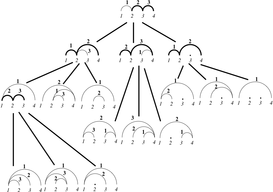
Figure 1. This is an $\mathcal{S}$-reduction tree with root labeled by $G^{\mathcal{S}}[x_{12}x_{23}x_{34}]$, when the edge-labels are disregarded. The boldface edges indicate where the reduction is performed. We can read off the following reduced form of $x_{12}x_{23}x_{34}$ from the set of leaves: $x_{14}x_{13}x_{12}+x_{14}x_{23}x_{13}+\beta x_{14}x_{13}+x_{24}x_{14}x_{23}+\beta x_{14}x_{23}+x_{34}x_{14}x_{12}+x_{34}x_{24}x_{14}+\beta x_{34}x_{14}+\beta x_{14}x_{12}+\beta x_{24}x_{14}+\beta^{2}x_{14}$. When the edge-labels are taken into account, this is the $\mathcal{B}$-reduction tree corresponding to equation (3). Note that in the second child of the root we commuted edge-labels 1 and 2.

Let $T$ be a noncrossing tree on the vertex set $[n+1]$. In terms of reduction trees, Theorem 2 states that the number of leaves labeled by graphs with exactly $n$ edges of an $\mathcal{S}$-reduction tree with root labeled $T$ is independent of the particular $\mathcal{S}$-reduction tree. The generalization of Theorem 2 for any $\beta$ states that the number leaves labeled by graphs with exactly $k$ edges of an $\mathcal{S}$-reduction tree with root labeled $T$, is independent of the particular $\mathcal{S}$-reduction tree for any $k$. In terms of reduced forms we can write this as follows. If $P_{n}^{\mathcal{S}}$ is the reduced form of a monomial $m^{\mathcal{S}}[T]$ for a noncrossing tree $T$, then

$$P_{n}^{\mathcal{S}}(x_{ij}=1)=\sum_{m=0}^{n-1}f_{T,n-m}\beta^{m},$$

where $f_{T,k}$ denotes the number of noncrossing alternating spanning forests of $\overline{T}$ with $k$ edges and additional technical requirements detailed in Section 8. Also, if $P_{n}^{\mathcal{B}}$ is the reduced form of a monomial $m^{\mathcal{B}}[T]$ for a noncrossing good tree $T$ (defined in Section 6), then

$$P^{\mathcal{B}}_{n}(x_{ij})=\sum_{F}x^{F},$$

where the sum runs over all noncrossing alternating spanning forests $F$ of $\overline{T}$ with lexicographic edge-labels (defined in Section 7) and additional technical requirements detailed in Section 8.

If we consider the reduced forms of the path monomial $w=\prod_{i=1}^{n}x_{i,i+1}$, then $T=P=([n+1],\{(i,i+1)\mid i\in[n]\})$, and $f_{P,k}$ is simply the number of noncrossing alternating spanning forests on $[n+1]$ with $k$ edges containing edge $(1,n+1)$. Furthermore, $P^{\mathcal{B}}_{n}(x_{ij})=\sum_{F}x^{F},$ where the sum runs over all noncrossing alternating spanning forests $F$ on $[n+1]$ with lexicographic edge-labels and containing edge $(1,n+1)$. See Section 7 for the treatment of this special case.

3. Acyclic root polytopes

In the terminology of [P], a root polytope of type $A_{n}$ is the convex hull of the origin and some of the points $e_{i}-e_{j}$ for $1\leq i<j\leq n+1$, where $e_{i}$ denotes the $i^{th}$ coordinate vector in $\mathbb{R}^{n+1}$. A very special root polytope is the full root polytope

$$\mathcal{P}(A_{n}^{+})=\textrm{ConvHull}(0,e_{ij}^{-}\mid 1\leq i<j\leq n+1),$$

where $e_{ij}^{-}=e_{i}-e_{j}$. We study a class of root polytopes including $\mathcal{P}(A_{n}^{+})$, which we now discuss.

Let $G$ be a graph on the vertex set $[n+1]$. Define

$$\mathcal{V}_{G}=\{e_{ij}^{-}\mid(i,j)\in E(G),i<j\},\mbox{ a set of vectors associated to $G$;}$$

$$\mathcal{C}(G)=\langle\mathcal{V}_{G}\rangle:=\{\sum_{e_{ij}^{-}\in\mathcal{V}_{G}}c_{ij}e_{ij}^{-}\mid c_{ij}\geq 0\},\mbox{ the cone associated to $G$; and }$$

$$\overline{\mathcal{V}}_{G}=\Phi^{+}\cap\mathcal{C}(G),\mbox{ all the positive roots of type $A_{n}$ contained in $\mathcal{C}(G)$},$$

where $\Phi^{+}=\{e_{ij}^{-}\mid 1\leq i<j\leq n+1\}$ is the set of positive roots of type $A_{n}$. The idea to consider the positive roots of a root system inside a cone appeared earlier in Reiner’s work [R1], [R2] on signed posets.

The root polytope $\mathcal{P}(G)$ associated to graph $G$ is

(5) $$\mathcal{P}(G)=\textrm{ConvHull}(0,e_{ij}^{-}\mid e_{ij}^{-}\in\overline{\mathcal{V}}_{G})$$

The root polytope $\mathcal{P}(G)$ associated to graph $G$ can also be defined as

(6) $$\mathcal{P}(G)=\mathcal{P}(A_{n}^{+})\cap\mathcal{C}(G).$$

The equivalence of these two definition is proved in Lemma 7 in Section 4.

Note that $\mathcal{P}(A_{n}^{+})=\mathcal{P}(P)$ for the path graph $P=([n+1],\{(i,i+1)\mid i\in[n]\}).$ While the choice of $G$ such that $\mathcal{P}(A_{n}^{+})=\mathcal{P}(G)$ is not unique, it becomes unique if we require that $G$ is minimal, that is for no edge $(i,j)\in E(G)$ can the corresponding vector $e_{ij}^{-}$ be written as a nonnegative linear combination of the vectors corresponding to the edges $E(G)\backslash\{e\}$. Graph $P$ is minimal.

We can describe the vertices in $\overline{\mathcal{V}}_{G}$ in terms of paths in $G$. A playable route of a graph $G$ is an ordered sequence of edges $(i_{1},j_{1}),(i_{2},j_{2}),\ldots,(i_{l},j_{l})\in E(G)$ such that $i_{1}<j_{1}=i_{2}<j_{2}\ldots j_{l-1}=i_{l}<j_{l}$.

Lemma 4.

Let $G$ be a graph on the vertex set $[n+1]$. Any $v\in\overline{\mathcal{V}}_{G}$ is $v=e_{i_{1}}-e_{j_{l}}$ for some playable route $(i_{1},j_{1}),(i_{2},j_{2}),\ldots,(i_{l},j_{l})$ of $G$. If in addition $G$ is acyclic, then the correspondence between playable routes of $G$ and vertices in $\overline{\mathcal{V}}_{G}$ is a bijection.

The proof of Lemma 4 is straightforward, and is left to the reader.

Define

$$\mathcal{L}_{n}=\{G=([n+1],E(G))\mid\mbox{ $G$ is an acyclic graph}\},$$

and

$$\mathcal{L}(A_{n}^{+})=\{\mathcal{P}(G)\mid G\in\mathcal{L}_{n}\},\mbox{the set of {acyclic root polytopes}.}$$

Note that the condition that $G$ is an acyclic graph is equivalent to $\mathcal{V}_{G}$ being a set of linearly independent vectors.

The full root polytope $\mathcal{P}(A_{n}^{+})\in\mathcal{L}(A_{n}^{+})$, since the path graph $P$ is acyclic. We show below how to obtain central triangulations for all polytopes $\mathcal{P}\in\mathcal{L}(A_{n}^{+})$. A central triangulation of a $d$-dimensional root polytope $\mathcal{P}$ is a collection of $d$-dimensional simplices with disjoint interiors whose union is $\mathcal{P}$, the vertices of which are vertices of $\mathcal{P}$ and the origin is a vertex of all of them. Depending on the context we at times take the intersections of these maximal simplices to be part of the triangulation.

We now state the crucial lemma which relates root polytopes and algebras $\mathcal{S}(A_{n})$ and $\mathcal{B}(A_{n})$ defined in Section 1.

Lemma 5.

(Reduction Lemma) Given a graph $G_{0}\in\mathcal{L}_{n}$ with $d$ edges let $(i,j),(j,k)\in E(G_{0})$ for some $i<j<k$ and $G_{1},G_{2},G_{3}$ as described by equations (2). Then $G_{1},G_{2},G_{3}\in\mathcal{L}_{n}$,

$$\mathcal{P}(G_{0})=\mathcal{P}(G_{1})\cup\mathcal{P}(G_{2})$$

where all polytopes $\mathcal{P}(G_{0}),\mathcal{P}(G_{1}),\mathcal{P}(G_{2})$ are $d$-dimensional and

$$\mathcal{P}(G_{3})=\mathcal{P}(G_{1})\cap\mathcal{P}(G_{2})\mbox{ is $(d-1)$-dimensional. }$$

What the Reduction Lemma really says is that performing a reduction on graph $G_{0}\in\mathcal{L}_{n}$ is the same as “cutting” the $d$-dimensional polytope $\mathcal{P}(G_{0})$ into two $d$-dimensional polytopes $\mathcal{P}(G_{1})$ and $\mathcal{P}(G_{2})$, whose vertex sets are subsets of the vertex set of $\mathcal{P}(G_{0})$, whose interiors are disjoint, whose union is $\mathcal{P}(G_{0})$, and whose intersection is a facet of both. We prove the Reduction Lemma in Section 4.

4. The proof of the Reduction Lemma

This section is devoted to proving the Reduction Lemma (Lemma 5). As we shall see in Section 5, the Reduction Lemma is the “secret force” that makes everything fall into its place for acyclic root polytopes. We start by providing a simple lemma which characterizes the root polytopes which are simplices, then in Lemma 7 we prove that equations (5) and (6) are equivalent definitions for the root polytope $\mathcal{P}(G)$, and finally we prove the Cone Reduction Lemma (Lemma 8), which, together with Lemma 7 implies the Reduction Lemma.

Lemma 6 is implied by the results in [P, Lemma 13.2], but for the sake of completeness we provide a proof of it. Note that the exact definitions and notations in [P] are different from ours. The idea for part of the proof of Lemma 7 appears in [P, F] with different purposes.

Lemma 6.

(Cf. [P, Lemma 13.2]) For a graph $G$ on $[n+1]$ vertices and $d$ edges, the polytope $\mathcal{P}(G)$ is a simplex if and only if $G$ is alternating and acyclic. If $\mathcal{P}(G)$ is a simplex, then its $d$-dimensional normalized volume $\mbox{\em vol}_{d}\,\mathcal{P}(G)=\frac{1}{d!}.$

Proof.

It follows from equation (5) that for a minimal graph $G$ the polytope $\mathcal{P}(G)$ is a simplex if and only if the vectors corresponding to the edges of $G$ are linearly independent and $\mathcal{C}(G)\cap\Phi^{+}=\mathcal{V}_{G}$.

The vectors corresponding to the edges of $G$ are linearly independent if and only if $G$ is acyclic. By Lemma 4, $\mathcal{C}(G)\cap\Phi^{+}=\mathcal{V}_{G}$ if and only if $G$ contains no edges $(i,j),(j,k)$ with $i<j<k$, i.e. $G$ is alternating.

That $\mbox{\rm vol}_{d}\,\mathcal{P}(G)=\frac{1}{d!}$ follows from the unimodality of $\Phi^{+}$.

∎

Lemma 7.

For any graph $G$ on the vertex set $[n+1]$,

$$\emph{ConvHull}(0,e_{ij}^{-}\mid e_{ij}^{-}\in\overline{\mathcal{V}}_{G})=\mathcal{P}(A_{n}^{+})\cap\mathcal{C}(G).$$

Proof.

For a graph $H$ on the vertex set $[n+1]$, let $\sigma(H)=\textrm{ConvHull}(0,e_{ij}^{-}\mid(i,j)\in H,i<j)$. Then, by Lemma 4, $\sigma(\overline{G})=\textrm{ConvHull}(0,e_{ij}^{-}\mid e_{ij}^{-}\in\overline{\mathcal{V}}_{G})$. Let $\sigma(\overline{G})$ be a $d$-dimensional polytope for some $d\leq n$ and consider any central triangulation of it: $\sigma(\overline{G})=\cup_{F\in\mathcal{F}}\sigma(F)$, where $\{\sigma(F)\}_{F\in\mathcal{F}}$ is a set of $d$-dimensional simplices with disjoint interiors, $E(F)\subset E(\overline{G})$, $F\in\mathcal{F}$. Since $\sigma(\overline{G})=\cup_{F\in\mathcal{F}}\sigma(F)$ is a central triangulation, it follows that $\sigma(F)=\sigma(\overline{G})\cap\mathcal{C}(F)$, for $F\in\mathcal{F}$, and $\mathcal{C}(G)=\cup_{F\in\mathcal{F}}\mathcal{C}(F)$.

Since $\sigma(F)$, $F\in\mathcal{F}$, is a $d$-dimensional simplex, it follows that $F$ is a forest with $d$ edges. Furthermore, $F\in\mathcal{F}$ is an alternating forest, as otherwise $(i,j),(j,k)\in E(F)\subset E(\overline{G})$, for some $i<j<k$ and while $e_{ik}^{-}=e_{ij}^{-}+e_{jk}^{-}\in\sigma(\overline{G})\cap\mathcal{C}(F)$, $e_{ik}^{-}\not\in\sigma(F)$, contradicting that $\cup_{F\in\mathcal{F}}\sigma(F)$ is a central triangulation of $\sigma(\overline{G})$. Thus, $\overline{F}=F$, and $\sigma(F)=\sigma(\overline{F})$. It is clear that $\sigma(\overline{F})=\textrm{ConvHull}(0,e_{ij}^{-}\mid e_{ij}^{-}\in\overline{\mathcal{V}}_{F})\subset\mathcal{P}(A_{n}^{+})\cap\mathcal{C}(F),$ $F\in\mathcal{F}$. Since if $x=(x_{1},\ldots,x_{n+1})$ is in the facet of $\sigma(\overline{F})$ opposite the origin, then $|x_{1}|+\cdots+|x_{n+1}|=2$ and for any point $x=(x_{1},\ldots,x_{n+1})\in\mathcal{P}(A_{n}^{+})$, $|x_{1}|+\cdots+|x_{n+1}|\leq 2$ it follows that $\mathcal{P}(A_{n}^{+})\cap\mathcal{C}(F)\subset\sigma(\overline{F})$. Thus, $\sigma(\overline{F})=\mathcal{P}(A_{n}^{+})\cap\mathcal{C}(F)$. Finally, $\textrm{ConvHull}(0,e_{ij}^{-}\mid e_{ij}^{-}\in\overline{\mathcal{V}}_{G})=\sigma(\overline{G})=\cup_{F\in\mathcal{F}}\sigma(F)=\cup_{F\in\mathcal{F}}\sigma(\overline{F})=\cup_{F\in\mathcal{F}}(\mathcal{P}(A_{n}^{+})\cap\mathcal{C}(F))=\mathcal{P}(A_{n}^{+})\cap(\cup_{F\in\mathcal{F}}\mathcal{C}(F))=\mathcal{P}(A_{n}^{+})\cap\mathcal{C}(G)$ as desired.

∎

Lemma 8.

(Cone Reduction Lemma) Given a graph $G_{0}\in\mathcal{L}_{n}$ with $d$ edges, let $G_{1},G_{2},G_{3}$ be the graphs described as by equations (2). Then $G_{1},G_{2},G_{3}\in\mathcal{L}_{n}$,

$$\mathcal{C}(G_{0})=\mathcal{C}(G_{1})\cup\mathcal{C}(G_{2})$$

where all cones $\mathcal{C}(G_{0}),\mathcal{C}(G_{1}),\mathcal{C}(G_{2})$ are $d$-dimensional and

$$\mathcal{C}(G_{3})=\mathcal{C}(G_{1})\cap\mathcal{C}(G_{2})\mbox{ is $(d-1)$-dimensional. }$$

Proof.

Let the edges of $G_{0}$ be $f_{1}=(i,j),f_{2}=(j,k),f_{3},\ldots,f_{d}$. Let ${\rm v}(f_{1}),$ ${\rm v}(f_{2}),$ ${\rm v}(f_{3}),\ldots,{\rm v}(f_{d})$ denote the vectors the edges of $G_{0}$ correspond to under the correspondence ${\rm v}:(i,j)\mapsto e_{ij}^{-}$, where $i<j$. Since $G_{0}\in\mathcal{L}_{n}$, the vectors ${\rm v}(f_{1}),{\rm v}(f_{2}),{\rm v}(f_{3}),\ldots,{\rm v}(f_{d})$ are linearly independent. By equations (2), $\mathcal{C}(G_{0})=\langle{\rm v}(f_{1}),{\rm v}(f_{2}),{\rm v}(f_{3}),\ldots,{\rm v}(f_{d})\rangle$, $\mathcal{C}(G_{1})=\langle{\rm v}(f_{1}),{\rm v}(f_{1})+{\rm v}(f_{2}),{\rm v}(f_{3}),\ldots,{\rm v}(f_{d})\rangle$, $\mathcal{C}(G_{2})=\langle{\rm v}(f_{1})+{\rm v}(f_{2}),{\rm v}(f_{2}),$ ${\rm v}(f_{3}),\ldots,{\rm v}(f_{d})\rangle$,

$\mathcal{C}(G_{3})=\langle{\rm v}(f_{1})+{\rm v}(f_{2}),{\rm v}(f_{3}),\ldots,{\rm v}(f_{d})\rangle$. Thus, $G_{1},G_{2},G_{3}\in\mathcal{L}_{n}$, cones $\mathcal{C}(G_{0}),\mathcal{C}(G_{1})$ and $\mathcal{C}(G_{2})$ are $d$-dimensional, while cone $\mathcal{C}(G_{3})$ is $(d-1)$-dimensional.

Clearly, $\mathcal{C}(G_{1})\cup\mathcal{C}(G_{2})\subset\mathcal{C}(G_{0})$. Any vector $v\in\mathcal{C}(G_{0})$ expressed in the basis ${\rm v}(f_{1}),{\rm v}(f_{2}),{\rm v}(f_{3}),\ldots,{\rm v}(f_{d})$ satisfies either $[{\rm v}(f_{1})]v\geq[{\rm v}(f_{2})]v$ or $[{\rm v}(f_{1})]v<[{\rm v}(f_{2})]v$. Thus, if $v\in\mathcal{C}(G_{0})$, then $v\in\mathcal{C}(G_{1})$ or $v\in\mathcal{C}(G_{2})$. Therefore, $\mathcal{C}(G_{0})=\mathcal{C}(G_{1})\cup\mathcal{C}(G_{2})$.

Clearly, $\mathcal{C}(G_{3})\subset\mathcal{C}(G_{1})\cap\mathcal{C}(G_{2})$. Any $v\in\mathcal{C}(G_{1})$ expressed in the basis ${\rm v}(f_{1}),{\rm v}(f_{2}),{\rm v}(f_{3}),\ldots,{\rm v}(f_{d})$ satisfies $[{\rm v}(f_{1})]v\geq[{\rm v}(f_{2})]v$, while $v\in\mathcal{C}(G_{2})$ expressed in the basis ${\rm v}(f_{1}),{\rm v}(f_{2}),{\rm v}(f_{3}),\ldots,{\rm v}(f_{d})$ satisfies $[{\rm v}(f_{1})]v\leq[{\rm v}(f_{2})]v$. Thus, $v\in\mathcal{C}(G_{1})\cap\mathcal{C}(G_{2})$ expressed in the basis ${\rm v}(f_{1}),{\rm v}(f_{2}),{\rm v}(f_{3}),\ldots,{\rm v}(f_{d})$ satisfies $[{\rm v}(f_{1})]v=[{\rm v}(f_{2})]v$. Therefore, $\mathcal{C}(G_{1})\cap\mathcal{C}(G_{2})\subset\mathcal{C}(G_{3})$, leading to $\mathcal{C}(G_{1})\cap\mathcal{C}(G_{2})=\mathcal{C}(G_{3})$. ∎

Proof of the Reduction Lemma (Lemma 5). Straightforward corollary of Lemmas 7 and 8.∎

In Section 5 we use Lemmas 5 and 6 to prove general theorems about acyclic root polytopes, which can be specialized to yield proofs of parts of Theorems 1 and 2.

5. General theorems for acyclic root polytopes

In this section we prove general theorems about acyclic root polytopes and reduced forms of monomials $m^{\mathcal{S}}[F]$, for a forest $F$.

Given a polytope $\mathcal{P}\subset\mathbb{R}^{n+1}$, the $t^{th}$ dilate of $\mathcal{P}$ is

$$t\mathcal{P}=\{(tx_{1},\ldots,tx_{n+1})|(x_{1},\ldots,x_{n+1})\in\mathcal{P}\}.$$

The Ehrhart polynomial of an integer polytope $\mathcal{P}\subset\mathbb{R}^{n+1}$ is

$$L_{\mathcal{P}}(t)=\#(t\mathcal{P}\cap\mathbb{Z}^{n+1}).$$

For background on the theory of Ehrhart polynomials see [BR].

Lemma 9.

Let $\mathcal{P}(G)^{\circ}=\bigsqcup_{\sigma^{\circ}\in S}\sigma^{\circ}$, where $S$ is a collection of open simplices $\sigma^{\circ}$, such that the origin is a vertex of each simplex in $S$ and the other vertices are from $\Phi^{+}$. Then the number of $i$-dimensional open simplices in $S$, denoted by $f_{i}$, only depends on $\mathcal{P}(G)$, not on $S$ itself.

Proof.

Since $\displaystyle\mathcal{P}(G)^{\circ}=\bigsqcup_{\sigma^{\circ}\in S}\sigma^{\circ}$, we have that $\displaystyle L_{\mathcal{P}(G)^{\circ}}(t)=\sum_{\sigma^{\circ}\in S}L_{\sigma^{\circ}}(t)$. Since the vectors in $\Phi^{+}$ are unimodular, it follows that for a $d$-dimensional simplex $\sigma^{\circ}\in S$, $L_{\sigma^{\circ}}(t)=L_{\Delta^{\circ}}(t)$, where $\Delta$ is the standard $d$-simplex. By [BR, Theorem 2.2] $L_{\Delta^{\circ}}(t)={t-1\choose d}.$ Thus,

$$L_{\mathcal{P}(G)^{\circ}}(t)=\sum_{i=0}^{\infty}f_{i}{t-1\choose i},$$

where $L_{\mathcal{P}(G)^{\circ}}(t)\in\mathbb{Z}[t]$ and the set $\{{t-1\choose i}\mid i=0,1,\ldots\}$ is a basis of $\mathbb{Z}[t]$. Therefore, $f_{i}$ are uniquely determined for $i=0,1,\ldots$, by $\mathcal{P}(G)$ and are independent of $S$. ∎

Theorem 10.

Let $F$ be any forest on the vertex set $[n+1]$ with $l$ edges. If $\mathcal{T}_{F}^{\mathcal{S}}$ is an $\mathcal{S}$-reduction tree with root labeled $F$, then the number of leaves of $\mathcal{T}_{F}^{\mathcal{S}}$ labeled by forests with $k$ edges, denoted by $f_{F,k}$, is a function of $F$ and $k$ only.

In other words, if $P^{\mathcal{S}}_{n}$ is a reduced form of $m^{\mathcal{S}}[F]$, then

$$P^{\mathcal{S}}_{n}(x_{ij}=1)=\sum_{l=0}^{l-1}f_{F,l-m}\beta^{m}.$$

Proof.

Let $\mathcal{T}_{F}^{\mathcal{S}}$ be a particular $\mathcal{S}$-reduction tree with root labeled $F$. By definition, the leaves of $\mathcal{T}_{F}^{\mathcal{S}}$ are labeled by alternating forests with $k$ edges, where $k\in[l]$. Let the $c_{k}$ forests $F^{k}_{1},\ldots,F^{k}_{c_{k}}$ label the leaves of $\mathcal{T}_{F}^{\mathcal{S}}$ with $k$ edges, $k\in[l]$. Repeated use of the Reduction Lemma (Lemma 5) implies that

(7) $$\mathcal{P}(F)^{\circ}=\bigsqcup_{k\in[l],i_{k}\in[c_{k}]}\mathcal{P}(F^{k}_{i_{k}})^{\circ},$$

where the right hand side is a disjoint union of simplices by Lemma 6. By Lemma 9, the number of $k$-dimensional simplices among $\bigcup_{k\in[l],i_{k}\in[c_{k}]}\{\mathcal{P}(F^{k}_{i_{k}})^{\circ}\}$ is independent of the particular $\mathcal{S}$-reduction tree $\mathcal{T}_{F}^{\mathcal{S}}$. Thus, $f_{T,k}=c_{k}$ only depends on $F$ and $k$.

The formula for the reduced form of $m^{\mathcal{S}}[F]$ evaluated at $x_{ij}=1$ follows from the correspondence between the leaves of $\mathcal{T}_{F}^{\mathcal{S}}$ and reduced forms described in Section 2.

∎

We easily obtain the Ehrhart polynomial, and thus also the volume of the polytope ${\mathcal{P}(F)}$ with the techniques used above.

Theorem 11.

The Ehrhart polynomial of the polytope ${\mathcal{P}(F)}$, where $F$ is a forest on the vertex set $[n+1]$ with $l$ edges, is

$$L_{\mathcal{P}(F)}(t)=(-1)^{l}\sum_{i=0}^{l}(-1)^{i}f_{F,i}{t+i\choose i},$$

where $f_{F,k}$ is the number of leaves of $\mathcal{T}_{F}^{\mathcal{S}}$ labeled by forests with $k$ edges.

Proof.

It follows from the proofs of Lemma 9 and Theorem 10 that

$$L_{\mathcal{P}(F)^{\circ}}(t)=\sum_{i=0}^{l}f_{F,i}{t-1\choose i}.$$

Since by the Ehrhart-Macdonald reciprocity [BR, Theorem 4.1]

$$L_{\mathcal{P}(F)}(t)=(-1)^{\dim\mathcal{P}(F)}L_{\mathcal{P}(F)^{\circ}}(-t),$$

it follows that

$$L_{\mathcal{P}(F)}(t)=(-1)^{l}\sum_{i=0}^{l}f_{F,i}{-t-1\choose i}=(-1)^{l}\sum_{i=0}^{l}(-1)^{i}f_{F,i}{t+i\choose i}.$$

∎

Corollary 12.

If $F$ is a forest on the vertex set $[n+1]$ with $l$ edges, then

$$\mbox{\rm vol}\,\mathcal{P}(F)=\frac{f_{F,l}}{l!}.$$

Proof.

By [BR, Lemma 3.19] the leading coefficient of $L_{\mathcal{P}(F)}(t)$ is equal to $\mbox{\rm vol}\,\mathcal{P}(F)$. We also obtain $\mbox{\rm vol}\,\mathcal{P}(F)=\frac{f_{F,l}}{l!}$ directly from the Reduction Lemma if we count the $l$-dimensional simplices in the triangulation of $\mathcal{P}(F)$.

∎

6. Reductions in the noncommutative case

In this section we prove two crucial lemmas about reduction (1) in the noncommutative case necessary for proving Theorem 2. While in the commutative case reductions on $G^{\mathcal{S}}[m]$ could result in crossing graphs, we prove that in the noncommutative case exactly those reductions from the commutative case are allowed which result in no crossing graphs, provided that $m=m^{\mathcal{B}}[T]$ for a noncrossing tree $T$ with suitable edge labels specified below. Furthermore, we also show that if there are any two edges $(i,j)$ and $(j,k)$ with $i<j<k$ in a successor of $G^{\mathcal{B}}[m]$, then after suitably many commutations it is possible to apply reduction (1). Thus, once the reduction process terminates, the set of graphs obtained as leaves of the reduction tree are alternating forests. Now, unlike in the commutative case, they are also noncrossing. In fact, each noncrossing alternating spanning forest of $\overline{T}$ satisfying certain additional technical conditions occurs among the leaves of the reduction tree exactly once, yielding a complete combinatorial description of the reduced form of $m^{\mathcal{B}}[T]$.

In terms of graphs the partial commutativity means that if $G$ contains two edges $(i,j)_{a}$ and $(k,l)_{a+1}$ with $i,j,k,l$ distinct, then we can replace these edges by $(i,j)_{a+1}$ and $(k,l)_{a}$, and vice versa. Reduction rule (1) on the other hand means that if there are two edges $(i,j)_{a}$ and $(j,k)_{a+1}$ in $G_{0}$, $i<j<k$, then we replace $G_{0}$ with three graphs $G_{1},G_{2},G_{3}$ on the vertex set $[n+1]$ and edge sets

$$E(G_{1}) = E(G_{0})\backslash\{(i,j)_{a}\}\backslash\{(j,k)_{a+1}\}\cup\{(i,k)_{a}\}\cup\{(i,j)_{a+1}\}$$

$$E(G_{2}) = E(G_{0})\backslash\{(i,j)_{a}\}\backslash\{(j,k)_{a+1}\}\cup\{(j,k)_{a}\}\cup\{(i,k)_{a+1}\}$$

(8) $$E(G_{3}) = (E(G_{0})\backslash\{(i,j)_{a}\}\backslash\{(j,k)_{a+1}\})^{a}\cup\{(i,k)_{a}\},$$

where $(E(G_{0})\backslash\{(i,j)_{a}\}\backslash\{(j,k)_{a+1}\})^{a}$ denotes the edges obtained from the edges $E(G_{0})\backslash\{(i,j)_{a}\}\backslash\{(j,k)_{a+1}\}$ by reducing the label of each edge which has label greater than $a$ by $1$.

A $\mathcal{B}$-reduction tree $\mathcal{T}^{\mathcal{B}}$ is defined analogously to an $\mathcal{S}$-reduction tree, except we use equation (6) to describe the children. See Figure 1 for an example. A graph $H$ is called a $\mathcal{B}$-successor of $G$ if it is obtained by a series of reductions from $G$. For convenience, we refer to commutativity of $x_{ij}$ and $x_{kl}$ for distinct $i,j,k,l$ as reduction (2), by which we mean the rule $x_{ij}x_{kl}\leftrightarrow x_{kl}x_{ij}$, for $i,j,k,l$ distinct, or, in the language of graphs, exchanging edges $(i,j)_{a}$ and $(k,l)_{a+1}$ with $(i,j)_{a+1}$ and $(k,l)_{a}$ for $i,j,k,l$ distinct.

A forest $H$ on the vertex set $[n+1]$ and $k$ edges labeled $1,\ldots,k$ is good if it satisfies the following conditions:

$(i)$ If edges $(i,j)_{a}$ and $(j,k)_{b}$ are in $H$, $i<j<k$, then $a<b$.

$(ii)$ If edges $(i,j)_{a}$ and $(i,k)_{b}$ in $H$ are such that $j<k$, then $a>b$.

$(iii)$ If edges $(i,j)_{a}$ and $(k,j)_{b}$ in $H$ are such that $i<k$, then $a>b$.

$(iv)$ $H$ is noncrossing.

No graph $H$ with a cycle could satisfy all of $(i),(ii),(iii),(iv)$ simultaneously, which is why we only define good forests. Note, however, that any forest $H$ has an edge-labeling that makes it a good forest.

Lemma 13.

If the root of an $\mathcal{B}$-reduction tree is labeled by a good forest, then all nodes of it are also labeled by good forests.

Proof.

The root of the $\mathcal{B}$-reduction tree is trivially labeled by a good forest. We show that after each reduction (1) or (2) all properties $(i),(ii),(iii),(iv)$ of good forests are preserved.

In reduction (2) we take disjoint edges $(i,j)_{a}$ and $(k,l)_{a+1}$ and replace them by the edges $(i,j)_{a+1}$ and $(k,l)_{a}$. It is easy to check that properties $(i),(ii),(iii),(iv)$ are preserved using the fact that all edge-labels are integers and are not repeated, so the relative orders of edge-labels for edges incident to the same vertex are unchanged.

Performing reduction (1) results in three new graphs as described by equation (6). It is easy to check that properties $(i),(ii),(iii)$ are preserved using the fact that all edge-labels are integers and are not repeated. To prove that property $(iv)$ is also preserved, note that by $(i),(ii),(iii)$ if edge $(i,j)$ is labeled $a$ and $(j,k)$ labeled $a+1$, then there cannot be edges with endpoint $j$ of the form $(i_{1},j)$ with $i_{1}<i$ or $(j,k_{1})$ with $k<k_{1}$, or else some of the conditions $(i),(ii),(iii)$ would be violated. That there is no edge of the form described in the previous sentence with endpoint $j$ together with the fact that the graph $G$ we applied reduction (1) to was noncrossing implies that edge $(i,k)$ does not cross any edges of $G$, and therefore the resulting graph is also noncrossing.

∎

A reduction applied to a noncrossing graph $G$ is noncrossing if the graphs resulting from the reduction are also noncrossing.

The following is then an immediate corollary of Lemma 13.

Corollary 14.

If $G$ is a good forest, then all reductions that can be applied to $G$ and its $\mathcal{B}$-successors are noncrossing.

Lemma 15.

Let $G$ be a good forest. Let $(i,j)_{a}$ and $(j,k)_{b}$ with $i<j<k$ be edges of $G$ such that no edge of $G$ crosses $(i,k)$. Then after finitely many applications of reduction (2) we can apply reduction (1) to edges $(i,j)$ and $(j,k)$.

Proof.

By the definition of a good forest it follows that $a<b$. If $b=a+1$, then we are done. Otherwise, consider all edges $(l,m)_{c}$ such that $a<c<b$. Since $G$ is a good forest and $(i,k)$ does not cross any edges of $G$, we find that for any such edge $(l,m)_{c}$ is either disjoint from edges $(i,j)_{a}$ and $(j,k)_{b}$, or else $(l,m)_{c}=(i,m)_{c}$ or $(l,m)_{c}=(l,k)_{c}$. Then reduction (2) can be applied to the edges $(l,m)_{c}$ with $a<c<b$ until either the edges labeled $a$ and $a+1$ or the edges labeled $b-1$ and $b$ are disjoint, in which case we can perform reduction (2) on these edges. Once this is done, the difference between the labels of the edges $(i,j)$ and $(j,k)$ decreased, and we can repeat this process until this difference is $1$, in which case reduction (1) can be applied to them. ∎

Corollary 16.

If $F$ labels a leaf of a $\mathcal{B}$-reduction tree whose root is labeled by a good forest, then $F$ is a good noncrossing alternating forest.

Proof.

By Lemma 13, $F$ is a good forest. By definition of good, it is also noncrossing. Lemma 15 implies that $F$ is alternating, or else reduction (1) could be applied to it, and thus it would not label a leaf of a $\mathcal{B}$-reduction tree. ∎

7. Proof of Theorems 1 and 2 in a special case

In this section we prove Theorems 1 and 2 for the special case where $T=P=([n+1],\{(i,i+1)\mid i\in[n]\}).$ We prove the general versions of the theorems in Section 8.

Given a noncrossing alternating forest $F$ on the vertex set $[n+1]$ with $k$ edges, the lexicographic order on its edges is as follows. Edge $(i_{1},j_{1})$ is less than edge $(i_{2},j_{2})$ in the lexicographic order if $j_{1}>j_{2}$, or $j_{1}=j_{2}$ and $i_{1}>i_{2}$. The forest $F$ is said to have lexicographic edge-labels if its edges are labeled with integers $1,\ldots,k$ such that if edge $(i_{1},j_{1})$ is less than edge $(i_{2},j_{2})$ in lexicographic order, then the label of $(i_{1},j_{1})$ is less than the label of $(i_{2},j_{2})$ in the usual order on the integers. Clearly, given any graph $G$ there is a unique edge-labeling of it which is lexicographic. Note that our definition of lexicographic is closely related to the conventional definition, but it is not exactly the same. For an example of lexicographic edge-labels, see the graphs labeling the leaves of the $\mathcal{B}$-reduction tree in Figure 1.

Lemma 17.

If a noncrossing alternating forest $F$ is a $\mathcal{B}$-successor of a good forest, then upon some number of reductions (2) performed on $F$, it is possible to obtain a noncrossing alternating forest $F^{\prime}$ with lexicographic edge-labels.

Proof.

If edges $e_{1}$ and $e_{2}$ of $F$ share a vertex and if $e_{1}$ is less than $e_{2}$ in the lexicographic order, then the label of $e_{1}$ is less than the label of $e_{2}$ in the usual order on integers by Lemma 13. Since reduction (2) swaps the labels of two vertex disjoint edges labeled by consecutive integers in a graph, these swaps do not affect the relative order of the labels on edges sharing vertices. Continue these swaps until the lexicographic order is obtained. ∎

To avoid confusion about whether the commutative or the noncommutative version of the problem is being considered, we denote $x_{12}x_{23}\cdots x_{n,n+1}$ by $w_{\mathcal{S}}$ in the commutative and by $w_{\mathcal{B}}$ in the noncommutative case.

Proposition 18.

By choosing the series of reductions suitably, the set of leaves of a $\mathcal{B}$-reduction tree with root labeled by $G^{\mathcal{B}}[w_{\mathcal{B}}]$ can be all noncrossing alternating forests $F$ on the vertex set $[n+1]$ containing edge $(1,n+1)$ with lexicographic edge-labels.

Proof.

By Corollary 16, all leaves of a $\mathcal{B}$-reduction tree are noncrossing alternating forests on the vertex set $[n+1]$. It is easily seen that they all contain edge $(1,n+1)$. By the correspondence between the leaves of a $\mathcal{B}$-reduction tree and simplices in a subdivision of $\mathcal{P}(G^{\mathcal{B}}[w_{\mathcal{B}}])$ obtained from the Reduction Lemma (Lemma 5), it follows that no forest appears more than once among the leaves. Thus, it suffices to prove that any noncrossing alternating forest $F$ on the vertex set $[n+1]$ containing edge $(1,n+1)$ appears among the leaves of a $\mathcal{B}$-reduction tree and that all these forests have lexicographic edge-labels. One can construct such a $\mathcal{B}$-reduction tree by induction on $n$. We show that starting with the path $(1,2),\ldots,(n,n+1)$ and performing reductions (1) and (2) we can obtain any noncrossing alternating forest $F$ on the vertex set $[n+1]$ containing edge $(1,n+1)$ with lexicographic edge-labels.

First perform the reductions on the path $(1,2),\ldots,(n,n+1)$ without involving edge $(n,n+1)$ in any of the reductions, until possible. Then we arrive to a set of trees where we have a noncrossing alternating forest $F$ on the vertex set $[n]$ containing edge $(1,n)$ with lexicographic labeling and in addition edge $(n,n+1)_{n}$. By inspection it follows that any noncrossing alternating forest $F$ on the vertex set $[n+1]$ containing edge $(1,n+1)$ with lexicographic edge-labels can be obtained from them. ∎

Theorem 19.

The set of leaves of a $\mathcal{B}$-reduction tree with root labeled by $G^{\mathcal{B}}[w_{\mathcal{B}}]$ is, up to applications of reduction (2), the set of all noncrossing alternating forests with lexicographic edge-labels on the vertex set $[n+1]$ containing edge $(1,n+1)$.

Proof.

By Proposition 18 there exists a $\mathcal{B}$-reduction tree which satisfies the conditions above. By Theorem 10 the number of forests with a fixed number of edges among the leaves of an $\mathcal{S}$-reduction tree is independent of the particular $\mathcal{S}$-reduction tree, and, thus, the same is true for a $\mathcal{B}$-reduction tree. It is clear that all forests labeling the leaves of a $\mathcal{B}$-reduction tree with root labeled by $G^{\mathcal{B}}[w_{\mathcal{B}}]$ have to contains the edge $(1,n+1)$. Also, no vertex-labeled forest, with edge-labels disregarded, can appear twice among the leaves of a $\mathcal{B}$-reduction tree. Together with Lemma 17 these imply the statement of Theorem 19. ∎

As corollaries of Theorem 19 we obtain the characterziation of reduced forms of the noncommutative monomial $w_{\mathcal{B}}$, as well as a way to calculate $f_{P,k}$, the number of forests with $k$ edges labeling the leaves of an $\mathcal{S}$-reduction tree $\mathcal{T}_{P}^{\mathcal{S}}$ with root labeled $P=([n+1],\{(i,i+1)\mid i\in[n]\}).$

Theorem 20.

If the polynomial $P^{\mathcal{B}}_{n}(x_{ij})$ is a reduced form of $w_{\mathcal{B}}$, then

$$P^{\mathcal{B}}_{n}(x_{ij})=\sum_{F}\beta^{n-|E(F)|}x^{F},$$

where the sum runs over all noncrossing alternating forests $F$ with lexicographic edge-labels on the vertex set $[n+1]$ containing edge $(1,n+1)$, and $x^{F}$ is defined to be the noncommutative monomial $\prod_{l=1}^{k}x_{i_{l},j_{l}}$ if $F$ contains the edges $(i_{1},j_{1})_{1},\ldots,(i_{k},j_{k})_{k}$.

Proposition 21.

The number of forests with $k$ edges labeling the leaves of an $\mathcal{S}$-reduction tree $\mathcal{T}_{P}^{\mathcal{S}}$, $f_{P,k}$, is equal to the number of noncrossing alternating forests on the vertex set $[n+1]$ and $k+1$ edges such that edge $(1,n+1)$ is present.

Proof.

Theorem 10 proves that number of leaves labeled by forests with $k$ edges in any $\mathcal{S}$-reduction tree with root labeled $P$ is independent of the particular $\mathcal{S}$-reduction tree. Since a $\mathcal{B}$-reduction tree becomes an $\mathcal{S}$-reduction tree when the edge-labels from the graphs labeling its nodes are deleted, the number of leaves labeled by forests with $k$ edges in any $\mathcal{S}$-reduction tree with root labeled $P$ is equal to the number of noncrossing alternating forests with lexicographic edge-labels on the vertex set $[n+1]$ with $k$ edges containing edge $(1,n+1)$ by Theorem 19.

∎

The Schröder numbers $s_{n}$ count the number of ways to draw any number of diagonals of a convex $(n+2)$-gon that do not intersect in their interiors. Let $s_{n,k}$ denote the number of ways to draw $k$ diagonals of a convex $(n+2)$-gon that do not intersect in their interiors. Cayley [C] in 1890 showed that $\displaystyle s_{n,k}=\frac{1}{n+1}{n+k+1\choose n}{n-1\choose k}$.

Lemma 22.

There is a bijection between the set of noncrossing alternating forests on the vertex set $[n+1]$ and $k+1$ edges such that edge $(1,n+1)$ is present and ways to draw $k$ diagonals of a convex $(n+2)$-gon that do not intersect in their interiors. Thus, $f_{P,k+1}=s_{n,k}$.

Proof.

The bijection can be described as follows. Given a forest $F$ with edges $(i_{1},j_{1}),\ldots,(i_{k},j_{k})$, $(1,n+1)$, correspond to it an $(n+2)$-gon on vertices $1,\ldots,n+2$ in a clockwise order, with diagonals $(i_{1},j_{1}+1),\ldots,(i_{k},j_{k}+1)$.

∎

Using $f_{P,k+1}=\frac{1}{n+1}{n+k+1\choose n}{n-1\choose k}$ we specialize Theorems 10 and 11 to Theorems 23 and 24.

Theorem 23.

If the polynomial $P^{\mathcal{S}}_{n}(x_{ij})$ is a reduced form of $w_{\mathcal{S}}$, then

$$P^{\mathcal{S}}_{n}(x_{ij}=1)=\sum_{m=0}^{n-1}s_{n,n-m-1}\beta^{m},$$

where $\displaystyle s_{n,k}=\frac{1}{n+1}{n+k+1\choose n}{n-1\choose k}$ is the number of noncrossing alternating forests on the vertex set $[n+1]$ with $k+1$ edges, containing edge $(1,n+1)$.

Theorem 24.

(Cf. [S3, Exercise 6.31], [F]) The Ehrhart polynomial of the polytope ${\mathcal{P}(A_{n}^{+})}$ is

$$L_{\mathcal{P}(A_{n}^{+})}(t)=\frac{(-1)^{n}}{n+1}\sum_{i=0}^{\infty}{n+i\choose n}{n-1\choose i-1}{-t-1\choose i}.$$

The generating function $J(\mathcal{P}(A_{n}^{+}),x)=1+\sum_{t=1}^{\infty}L_{\mathcal{P}(A_{n}^{+})}(t)x^{t}$ was previously calculated by different methods; see [S3, Exercise 6.31], [F].

8. Proof of Theorems 1 and 2 in the general case

In this section we find an analogue of Theorem 20 for any noncrossing good tree $T$, and using it calculate the numbers $f_{T,k}$. Specializing Theorems 10 and 11 to $T$, we then conclude the proofs of Theorems 1 and 2.

Theorems 20 and 23 imply Theorem 2 for the special case $T=P=([n+1],\{(i,i+1)\mid i\in[n]\}).$ We generalize Theorems 19, 20 and 23 to monomials $m^{\mathcal{B}}[T]$, where $T$ is a good tree. For this we need some technical definitions.

Consider a noncrossing tree $T$ on $[n+1]$. We define the pseudo-components of $T$ inductively. The unique simple path $P$ from $1$ to $n+1$ is a pseudo-component of $T$. The graph $T\backslash P$ is an edge-disjoint union of trees $T_{1},\ldots,T_{k}$, such that if $v$ is a vertex of $P$ and $v\in T_{l}$, $l\in[k]$, then $v$ is either the minimal or maximal vertex of $T_{l}$ . Furthermore, there are no $k-1$ trees whose edge-disjoint union is $T\backslash P$ and which satisfy all the requirements stated above. The set of pseudo-components of $T$, denoted by $ps(T)$ is $ps(T)=\{P\}\cup ps(T_{1})\cup\cdots\cup ps(T_{k})$. A pseudo-component $P^{\prime}$ is said to be on $[i,j]$, $i<j$ if it is a path with endpoints $i$ and $j$. A pseudo-component $P^{\prime}$ on $[i,j]$ is said to be a left pseudo-component of $T$ if there are no edges $(s,i)\in E(T)$ with $s<i$ and a right pseudo-component if if there are no edges $(j,s)\in E(T)$ with $j<s$. See Figure 2 for an example.

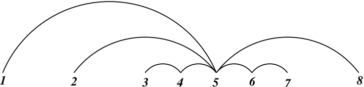
Figure 2. The edge sets of the pseudo-components in the graph depicted are $\{(1,5),(5,8)\},\{(2,5)\},\{(3,4),(4,5)\},\{(5,6),(6,7)\}$. The pseudo-component with edge set $\{(1,5),(5,8)\}$ is a both a left and right pseudo-component, while the pseudo-components with edge sets $\{(2,5)\},\{(3,4),(4,5)\}$ are left pseudo-components and the pseudo-component with edge set $\{(5,6),(6,7)\}$ is a right pseudo-component.

Proposition 25.

Let $T$ be a good tree. By choosing the series of reductions suitably, the set of leaves of a $\mathcal{B}$-reduction tree with root $T$ can be all noncrossing alternating spanning forests of $\overline{T}$ with lexicographic edge-labels on the vertex set $[n+1]$ containing edge $(1,n+1)$ and at least one edge of the form $(i_{1},j)$ with $i_{1}\leq i$ for each right pseudo-component of $T$ on $[i,j]$ and at least one edge of the form $(i,j_{1})$ with $j\leq j_{1}$ for each left pseudo-component of $T$ on $[i,j]$. See Figure 3 for an example.

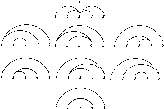
Figure 3. Trees $T_{1},\ldots,T_{6}$ as depicted in Figure 4 are the noncrossing alternating spanning trees of $\overline{T}$. This figure depicts all the other noncrossing alternating spanning forests of $\overline{T}$ on the vertex set $[n+1]$ containing edge $(1,n+1)$ and at least one edge of the form $(i_{1},j)$ with $i_{1}\leq i$ for each right pseudo-component of $T$ on $[i,j]$ and at least one edge of the form $(i,j_{1})$ with $j\leq j_{1}$ for each left pseudo-component of $T$ on $[i,j]$. By the Ehrhart polynomial form of Theorem 1, see end of Section 8, $L_{\mathcal{P}(T)}(t)={t+2\choose 2}-6{t+3\choose 3}+6{t+4\choose 4}$, since $f_{T,2}=1,f_{T,3}=6,f_{T,4}=6$ and $f_{T,i}=0$, for $i\neq 2,3,4$.

Proof.

It is easily seen that all graphs labeling the leaves of a $\mathcal{B}$-reduction tree must be noncrossing alternating spanning forests of $\overline{T}$ on the vertex set $[n+1]$ containing edge $(1,n+1)$ and at least one edge of the form $(i_{1},j)$ with $i_{1}\leq i$ for each right pseudo-component of $T$ on $[i,j]$ and at least one edge of the form $(i,j_{1})$ with $j\leq j_{1}$ for each left pseudo-component of $T$ on $[i,j]$. The proof then follows the proof of Proposition 18. To show that any noncrossing alternating spanning forests of $\overline{T}$ on the vertex set $[n+1]$ containing edge $(1,n+1)$ and at least one edge of the form $(i_{1},j)$ with $i_{1}\leq i$ for each right pseudo-component of $T$ on $[i,j]$ and at least one edge of the form $(i,j_{1})$ with $j\leq j_{1}$ for each left pseudo-component of $T$ on $[i,j]$ appears among the leaves of a $\mathcal{B}$-reduction tree and that all these forests have lexicographic edge-labels, we use induction on the number of pseudo-components of $T$. The base case is proved in Proposition 18. Suppose now that $T$ has $p$ pseudo-components, and let $P$ be such a pseudo-component that $T\backslash P$ is a tree with $p-1$ pseudo-components. Apply the inductive hypothesis to $T\backslash P$ and Proposition 18 to $P$ and combine the graphs obtained as outcomes in all the ways possible to obtain a set $S$ of graphs labeling the nodes of the reduction tree from which any leaf can be obtained by successive reductions. By inspection we see that any noncrossing alternating spanning forest of $\overline{T}$ on the vertex set $[n+1]$ containing edge $(1,n+1)$ and at least one edge of the form $(i_{1},j)$ with $i_{1}\leq i$ for each right pseudo-component of $T$ on $[i,j]$ and at least one edge of the form $(i,j_{1})$ with $j\leq j_{1}$ for each left pseudo-component of $T$ on $[i,j]$ can be obtained by reductions from the elements of $S$. Since no graph can be obtained twice, and no other graph can label a leaf of a $\mathcal{B}$-reduction, the proof is complete. ∎

Theorem 26.

Let $T$ be a good tree. The set of leaves of a $\mathcal{B}$-reduction tree with root labeled $T$ is, up to applications of reduction (2), the set of all noncrossing alternating spanning forests of $\overline{T}$ with lexicographic edge-labels on the vertex set $[n+1]$ containing edge $(1,n+1)$ and at least one edge of the form $(i_{1},j)$ with $i_{1}\leq i$ for each right pseudo-component of $T$ on $[i,j]$ and at least one edge of the form $(i,j_{1})$ with $j\leq j_{1}$ for each left pseudo-component of $T$ on $[i,j]$.

Proof.

The proof is analogous to that of Theorem 19 using Proposition 25 instead of Proposition 18.

∎

As corollaries of Theorem 26 we obtain the characterziation of reduced forms of the noncommutative monomial $m^{\mathcal{B}}[T]$ for a good tree $T$, as well as a combinatorial description of $f_{T,k}$, the number of forests with $k$ edges labeling the leaves of an $\mathcal{S}$-reduction tree $\mathcal{T}_{T}^{\mathcal{S}}$ with root labeled $T.$

Theorem 2. (Noncommutative part.) If the polynomial $P^{\mathcal{B}}_{n}(x_{ij})$ is a reduced form of $m^{\mathcal{B}}[T]$ for a good tree $T$, then

$$P^{\mathcal{B}}_{n}(x_{ij})=\sum_{F}\beta^{n-|E(F)|}x^{F},$$

where the sum runs over all noncrossing alternating spanning forests of $\overline{T}$ with lexicographic edge-labels on the vertex set $[n+1]$ containing edge $(1,n+1)$ and at least one edge of the form $(i_{1},j)$ with $i_{1}\leq i$ for each right pseudo-component of $T$ on $[i,j]$ and at least one edge of the form $(i,j_{1})$ with $j\leq j_{1}$ for each left pseudo-component of $T$ on $[i,j]$, and $x^{F}$ is defined to be the noncommutative monomial $\prod_{l=1}^{k}x_{i_{l},j_{l}}$ if $F$ contains the edges $(i_{1},j_{1})_{1},\ldots,(i_{k},j_{k})_{k}$.

Proposition 27.

Let $T$ be a good tree. The number of forests with $k$ edges labeling the leaves of an $\mathcal{S}$-reduction tree $\mathcal{T}_{T}^{\mathcal{S}}$ with root labeled by $T$, $f_{T,k}$, is equal to the number of noncrossing alternating spanning forests $F$ of $\overline{T}$ containing edge $(1,n+1)$ and at least one edge of the form $(i_{1},j)$ with $i_{1}\leq i$ for each right pseudo-component of $T$ on $[i,j]$ and at least one edge of the form $(i,j_{1})$ with $j\leq j_{1}$ for each left pseudo-component of $T$ on $[i,j]$.

Proposition 27 provides a combinatorial description of the coefficients in Theorems 10, 11 and Corollary 12, completing the proofs of Theorems 1 and 2. We state them in full generality here.

Theorem 2. (Commutative part.) If the polynomial $P^{\mathcal{S}}_{n}(x_{ij})$ is a reduced form of $m^{\mathcal{S}}[T]$ for a good tree $T$, then

$$P^{\mathcal{S}}_{n}(x_{ij}=1)=\sum_{l=0}^{l-1}f_{T,l-m}\beta^{m},$$

where $f_{T,k}$ is as in Proposition 27.

Theorem 1. (Ehrhart polynomial and volume.) The Ehrhart polynomial and volume of the polytope ${\mathcal{P}(T)}$, for a good tree $T$ on the vertex set $[n+1]$, are, respectively,

$$L_{\mathcal{P}(T)}(t)=(-1)^{n}\sum_{i=0}^{n}(-1)^{i}f_{T,i}{t+i\choose i},$$

$$\mbox{\rm vol}\,\mathcal{P}(T)=\frac{f_{T,n}}{n!},$$

where $f_{T,k}$ is as in Proposition 27. See Figure 3 for an example.

Theorem 1 can be generalized so that we not only describe the $n$-dimensional simplices in the triangulation of $\mathcal{P}(T)$, but also describe their intersections in terms of noncrossing alternating spanning forests in $\overline{T}$. Using the Reduction Lemma (Lemma 5) and Theorem 26 we can deduce the following.

Theorem 1. (Canonical triangulation.) If $T$ is a noncrossing tree on the vertex set $[n+1]$ and $T_{1},\ldots,T_{k}$ are the noncrossing alternating spanning trees of $\overline{T}$, then the root polytopes $\mathcal{P}(T_{1}),\ldots,\mathcal{P}(T_{k})$ are $n$-dimensional simplices forming a triangulation of $\mathcal{P}(T)$. Furthermore, the intersections of the top dimensional simplices $\mathcal{P}(T_{1}),\ldots,\mathcal{P}(T_{k})$ are simplices $\mathcal{P}(F)$, where $F$ run over all noncrossing alternating spanning forests of $\overline{T}$ with lexicographic edge-labels on the vertex set $[n+1]$ containing edge $(1,n+1)$and at least one edge of the form $(i_{1},j)$ with $i_{1}\leq i$ for each right pseudo-component of $T$ on $[i,j]$ and at least one edge of the form $(i,j_{1})$ with $j\leq j_{1}$ for each left pseudo-component of $T$ on $[i,j]$.

9. Properties of the canonical triangulation

In this section we show that the canonical triangulation of $\mathcal{P}(T)$ into simplices $\mathcal{P}(T_{1}),\ldots,\mathcal{P}(T_{k})$, and their faces, where $T_{1},\ldots,T_{k}$ are the noncrossing alternating spanning trees of $\overline{T}$, as described in Theorem 1, is regular and flag. We construct a shelling and using this shelling calculate the generating function $J(\mathcal{P}(T),x)=1+\sum_{t=1}^{\infty}L_{\mathcal{P}(T)}(t)x^{t}$, yielding another way to compute the Ehrhart polynomials. This generalizes the calculation of $J(\mathcal{P}(A_{n}^{+}),x)$, [S3, Exercise 6.31], [F].

Recall that a triangulation of the polytope $P$ is regular if there exists a concave piecewise linear function $f:P\rightarrow\mathbb{R}$ such that the regions of linearity of $f$ are the maximal simplices in the triangulation. It has been shown in [GGP, Theorem 6.3] that the noncrossing triangulation of $\mathcal{P}(A_{n}^{+})$ is regular. This result can be naturally extended to the canonical triangulation of any of the root polytopes $\mathcal{P}(T)$. An attractive proof uses the following concave function constructed by Postnikov for an alternative proof of [GGP, Theorem 6.3].

Let $f:A\rightarrow\mathbb{R}$ be a function on the set $A$ such that polytope $P={\rm ConvHull}(A)$. Let $\tilde{P}={\rm ConvHull}((a,f(a))\mid a\in A)$ and define then $f(p)={\rm max}\{x\mid\pi(a,x)=p,(a,x)\in\tilde{P}\}$, $p\in P$. The function $f:P\rightarrow\mathbb{R}$ is concave by definition. Consider the root polytope $\mathcal{P}(T)$ with vertices $0$ and $e_{i}-e_{j}$, where $(i,j)\in I\times J$. Let $f(0)=0$ and $f(e_{i}-e_{j})=(i-j)^{2}$ for $(i,j)\in I\times J$. Extend this to a concave piecewise linear function as explained in the above paragraph. A check of the regions of linearity proves the regularity of the canonical triangulation of $\mathcal{P}(T)$.

It can also be shown that the canonical triangulation of $\mathcal{P}(T)$ is flag, which we leave as an exercise to the reader. For the definition and importance of flag triangulations see [H, Section 2].

The canonical triangulation of $\mathcal{P}(T)$ is shellable, if there is a shelling, a linear order ${\rm v}(f_{1}),\ldots,F_{k}$ on $\mathcal{P}(T_{1}),\ldots,\mathcal{P}(T_{k})$, such that for all $2\leq i\leq k$, $F_{i}$ is attached to ${\rm v}(f_{1})\cup\ldots\cup F_{i-1}$ on a union of nonzero facets of $F_{i}$. See [S2] for more details.

The lexicographic ordering on the facets $\mathcal{P}(T_{1}),\ldots,\mathcal{P}(T_{k})$ is as follows: $\mathcal{P}(T_{i})<_{lex}\mathcal{P}(T_{j})$ if and only if for some $l$ the first $l$ edges of $T_{i}$ and $T_{j}$ in lexicographic ordering coincide and the $(l+1)^{st}$ edge of $T_{i}$ is less than the $(l+1)^{st}$ edge of $T_{j}$ in lexicographic ordering. The lexicographic ordering on the edges differs from the one we defined in Section 7; instead, here we use the conventional one. Namely, edge $(i_{1},j_{1})$ is less than edge $(i_{2},j_{2})$ in the lexicographic order if $i_{1}<i_{2}$, or $i_{1}=i_{2}$ and $j_{1}<j_{2}$.

Theorem 28.

Let $T$ be a noncrossing tree on the vertex set $[n+1]$. Let $T_{1},\ldots,T_{k}$ be the noncrossing alternating spanning trees of $\overline{T}$ such that $\mathcal{P}(T_{1})<_{lex}\cdots<_{lex}\mathcal{P}(T_{k})$. Then $\mathcal{P}(T_{1}),$ $\ldots,\mathcal{P}(T_{k})$ is a shelling order. See Figure 4 for an example.

Proof.

It suffices to show that for all $2\leq m\leq k$, the intersection $\mathcal{P}(T_{m})\cap(\mathcal{P}(T_{1})\cup\ldots\cup\mathcal{P}(T_{m-1}))$ is a union of nonzero facets of $\mathcal{P}(T_{m})$.

Let $L(T_{m})$ denote the set of left vertices of $T_{m}$, that is, the vertices of $T_{m}$ which are the smaller vertex of each edge incident to them. Let

$$S(T_{m})=\{(i,j)\mid i\in L(T_{m})\mbox{ and $j$ is the largest vertex adjacent to $i$ in $T_{m}$}\}.$$

The set $S(T_{m})$ uniquely determines $T_{m}$, since $T_{m}$ is a noncrossing alternating spanning tree.

There are exactly two noncrossing alternating trees containing $F=([n+1],E(T_{m})\backslash\{(i,j)\})$, $(i,j)\in S(T_{m})\backslash\{(1,n+1)\}$, namely, $T_{m}$ and $\tilde{T}_{m}=([n+1],E(F)\cup\{(i^{\prime},j^{\prime})\}),$ where $i^{\prime}$ is the biggest vertex of $T_{m}$ smaller than $i$ such that $(i^{\prime},j)\in E(T_{m}),$ and $j^{\prime}$ is the biggest vertex of $T_{m}$ smaller than $j$ such that $(i,j^{\prime})\in E(T_{m})$, or if $(i,j)$ is the only edge incident to $i$, then $j^{\prime}=i$. Let $f_{T_{m}}:S(T_{m})\backslash\{(1,n+1)\}\rightarrow E(K_{n+1})$ be defined by $f_{T_{m}}:(i,j)\mapsto(i^{\prime},j^{\prime})$ according to the rule explained above. Define

$$M_{T}(T_{m})=\{(i,j)\in S(T_{m})\mid f_{T_{m}}((i,j))\not\in\overline{T}\}.$$

The set $S_{T}(T_{m})=S(T_{m})\backslash M_{T}(T_{m})$ uniquely determines $T_{m}$, since $T_{m}$ is a noncrossing alternating spanning tree of $\overline{T}$. Furthermore, if for some $m^{\prime}\in[k]$, $m^{\prime}\neq m$, $S_{T}(T_{m})\subset E(T_{m^{\prime}})$, then $\mathcal{P}(T_{m})<_{lex}\mathcal{P}(T_{m^{\prime}})$. Thus, if for a forest $F$ on the vertex set $[n+1]$, $S_{T}(T_{m})\subset E(F)\subset E(T_{m})$, then $\mathcal{P}(F)$ is not a face of $\mathcal{P}(T_{1})\cup\ldots\cup\mathcal{P}(T_{m-1})$. If $F\subset T_{m}$ does not contain $S_{T}(T_{m})$ and $|E(F)|=n-1$, then $F\subset T_{l}=([n+1],E(T_{m})\backslash\{(i,j)\}\cup\{f_{T_{m}}((i,j))\})$ for $l<m$. Thus, for all $2\leq m\leq k$,

$$\mathcal{P}(T_{m})\cap(\mathcal{P}(T_{1})\cup\ldots\cup\mathcal{P}(T_{m-1}))=\bigcup_{(i,j)\in S_{T}(T_{m})}\mathcal{P}(([n+1],E(T_{m})\backslash\{(i,j)\})).$$

See Figure 4 for an example. ∎

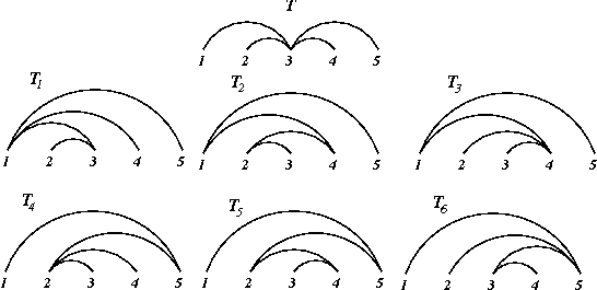
Figure 4. Trees $T_{1},\ldots,T_{6}$ are the noncrossing alternating spanning trees of $\overline{T}$. The root polytopes associated to them satisfy $\mathcal{P}(T_{1})<_{lex}\cdots<_{lex}\mathcal{P}(T_{6})$.
$S_{T}(T_{1})=\emptyset,S_{T}(T_{2})=\{(2,4)\},S_{T}(T_{3})=\{3,4\},\newline S_{T}(T_{4})=\{(2,5)\},S_{T}(T_{5})=\{(2,5),(3,4)\},S_{T}(T_{6})=\{(3,5)\}$.
By Theorem 29, $J(\mathcal{P}(T),x)=\displaystyle\frac{x^{2}+4x+1}{(1-x)^{5}}.$ This is of course equivalent to $L_{\mathcal{P}(T)}(t)={t+2\choose 2}-6{t+3\choose 3}+6{t+4\choose 4}$ as calculated in Figure 3. For a way to see this equivalence directly, see [BR, Lemma 3.14].

Theorem 29.

Let $T$ be a good tree on the vertex set $[n+1]$. Let $c(n,l)$ be the number of noncrossing alternating spanning trees $T_{m}$ of $\overline{T}$ with $|S_{T}(T_{m})|=l$. Then,

$$(1-x)^{n+1}J(\mathcal{P}(T),x)=\sum_{l=1}^{n}c(n,l-1)x^{l-1}.$$

Proof.

It can be seen that for a forest $F$ with $r$ edges, $J(\mathcal{P}(F),x)=\frac{1}{(1-x)^{r+1}},$ [BR, Theorem 2.2]. If we are adding the simplices $\mathcal{P}(T_{1}),\ldots,\mathcal{P}(T_{k})$ in lexicographic order one at a time, and calculating their contribution to $J(\mathcal{P}(T),x)$, then the contribution of $\mathcal{P}(T_{m})$ such that $\mathcal{P}(T_{m})\cap(\mathcal{P}(T_{1})\cup\ldots\cup\mathcal{P}(T_{m-1}))$ is a union of $(l-1)$ facets of $\mathcal{P}(T_{m})$ is

$$\frac{1}{(1-x)^{n+1}}-(l-1)\frac{1}{(1-x)^{n}}+\cdots+(-1)^{l-1}{l-1\choose l-1}\frac{1}{(1-x)^{n+1-(l-1)}}=\frac{x^{l-1}}{(1-x)^{n+1}}.$$

Hence,

$$J(\mathcal{P}(T),x)=\frac{\sum_{l=1}^{n}c(n,l-1)x^{l-1}}{(1-x)^{n+1}}.$$

∎

Remark.

All the theorems proved for trees (monomials corresponding to trees) in this paper can be formulated for forests (monomials corresponding to forests), and the proofs proceed analogously. The acyclic condition for graphs in the theorems is crucial for the proof techniques to work, but the noncrossing condition is not. Given an acyclic graph $G$ which is crossing, we can uncross it to obtain a new graph $G^{u}$. The graph $G^{u}$ is a noncrossing graph such that there is a graph isomorphism $\phi:G\rightarrow G^{u}$, where if $(i,j)\in E(G)$, $i<j$, then $\phi(i)<\phi(j)$. The graph $G^{u}$ is not uniquely determined by these conditions. All the results apply to any $G^{u}$, and they can be translated back for $G$ in an obvious way. E.g. the volume of $\mathcal{P}(T)$ for any tree $T$ on the vertex set $[n+1]$ is $\mbox{\rm vol}\,\mathcal{P}(T)=f_{T^{u}}\frac{1}{n!},$ where $f_{T^{u}}$ denotes the number of noncrossing alternating spanning trees of $\overline{T^{u}}$, the transitive closure of the uncrossed $T$.

10. Unique reduced forms and Gröbner bases

The reduced form of a monomial $m\in\mathcal{B}(A_{n})$ was defined in the Introduction as a polynomial $P_{n}^{\mathcal{B}}$ obtained by successive applications of the reduction rule (1) until no further reduction is possible, where we allow commuting any two variables $x_{ij}$ and $x_{kl}$ where $i,j,k,l$ are distinct, between the reductions. An alternative way of thinking of the reduced form of a monomial $m\in\mathcal{B}(A_{n})$ is to view the reduction process in $\mathbb{Q}\langle\beta,x_{ij}\mid 1\leq i<j\leq n\rangle/I_{\beta},$ where the generators of the (two-sided) ideal $I_{\beta}$ in $\mathbb{Q}\langle\beta,x_{ij}\mid 1\leq i<j\leq n+1\rangle$ are the elements $x_{ij}x_{kl}-x_{kl}x_{ij}$ for $i<j,k<l$ distinct, and $\beta x_{ij}-x_{ij}\beta$, $i<j$. In this section we prove the following theorem.

Theorem 30.

The reduced form of any monomial $m\in\mathcal{B}(A_{n})$ is unique.

We use noncommutative Gröbner bases techniques, which we now briefly review. We use the terminology and notation of [G], but state the results only for our special algebra. For the more general statements, see [G]. Throughout this section we consider the noncommutative case only.

Let

$${\bf R=\mathbb{Q}\langle\beta,x_{ij}\mid 1\leq i<j\leq n+1\rangle/I_{\beta}}$$

with multiplicative basis $\mathcal{B}$, the set of noncommutative monomials in variables $\beta$ and $x_{ij}$, where $1\leq i<j\leq n$, up to equivalence under the commutativity relations described by $I_{\beta}$.

The tip of an element $f\in R$ is the largest basis element appearing in its expansion, denoted by Tip$(f)$. Let CTip$(f)$ denote the coefficient of Tip$(f)$ in this expansion. A set of elements $X$ is tip reduced if for distinct elements $x,y\in X$, Tip$(x)$ does not divide Tip$(y)$.

A well-order $>$ on $\mathcal{B}$ is admissible if for $p,q,r,s\in\mathcal{B}$:

1. if $p<q$ then $pr<qr$ if both $pr\neq 0$ and $qr\neq 0$;

2. if $p<q$ then $sp<sq$ if both $sp\neq 0$ and $sq\neq 0$;

3. if $p=qr$, then $p>q$ and $p>r$.

Let $f,g\in R$ and suppose that there are monomials $b,c\in\mathcal{B}$ such that

1. Tip$(f)c$=$b$Tip$(g)$.

2. Tip$(f)$ does not divide $b$ and Tip$(g)$ does not divide $c.$

Then the overlap relation of $f$ and $g$ by $b$ and $c$ is

$$o(f,g,b,c)=\frac{fc}{\mbox{CTip}(f)}-\frac{bg}{\mbox{CTip}(g)}.$$

Proposition 31.

([G, Theorem 2.3]) A tip reduced generating set of elements $\mathcal{G}$ of the ideal $J$ of $R$ is a Gröbner basis, where the ordering on the monomials is admissible, if for every overlap relation

$$o(g_{1},g_{2},p,q)\Rightarrow_{\mathcal{G}}0,$$

where $g_{1},g_{2}\in\mathcal{G}$ and the above notation means that dividing $o(g_{1},g_{2},p,q)$ by $\mathcal{G}$ yields a remainder of $0$.

See [G, Theorem 2.3] for the more general formulation of Proposition 31 and [G, Section 2.3.2] for the formulation of the Division Algorithm.

Proposition 32.

Let $J$ be the ideal generated by the elements

$$x_{ij}x_{jk}-x_{ik}x_{ij}-x_{jk}x_{ik}-\beta x_{ik},\mbox{ for }1\leq i<j<k\leq n+1,$$

in $R$. Then there is a monomial order in which the above generators of $J$ form a Gröbner basis $\mathcal{G}$ of $J$ in $R$, and the tips of the generators are, $x_{ij}x_{jk}$.

Proof.

Let $x_{ij}>x_{kl}$ if $(i,j)$ is less than $(k,l)$ lexicographically. The degree of a monomial is determined by setting the degrees of $x_{ij}$ to be $1$ and the degrees of $\beta$ and scalars to be $0$. A monomial with higher degree is bigger in the order $>$, and the lexicographically bigger monomial of the same degree is greater than the lexicographically smaller one. Since in $R$ two equal monomials can be written in two different ways due to commutations, we can pick a representative to work with, say the one which is the “largest” lexicographically among all possible ways of writing the monomial, to resolve any ambiguities. The order $>$ just defined is admissible, and in it the tip of $x_{ij}x_{jk}-x_{ik}x_{ij}-x_{jk}x_{ik}-\beta x_{ik}$, for $1\leq i<j<k\leq n+1$, is $x_{ij}x_{jk}$. In particular, the generators of $J$ are tip reduced. A calculation of the overlap relations shows that $o(g_{1},g_{2},p,q)\Rightarrow_{\mathcal{G}}0$ in $R$, where $g_{1},g_{2}\in\mathcal{G}$. Proposition 31 then implies Proposition 32. ∎

Corollary 33.

The reduced form of a noncommutative monomial $m$ in variables $\beta$ and $x_{ij}$, $1\leq i<j\leq n+1$, is unique in $R$.

Proof.

Since the tips of elements of the Gröbner basis $\mathcal{G}$ of $J$ are exactly the monomials which we replace in the prescribed reduction rule (1), the reduced form of a monomial $m$ is the remainder $r$ upon division by the elements of $\mathcal{G}$ with the order $>$ described in the proof of Proposition 32. Since we proved that in $R$ the basis $\mathcal{G}$ is a Gröbner basis of $J$, it follows by [G, Proposition 2.7] that the remainder $r$ of the division of $m$ by $\mathcal{G}$ is unique in $R$. That is, the reduced form of a good monomial $m$ is unique in $R$. ∎

Note that Corollary 33 is equivalent to Theorem 30.

References

- [BR] M. Beck, S. Robins, Computing the continuous discretely, Springer Science + Business Media, LLCC, 2007.
- [C] A. Cayley, On the partitions of a polygon, Proc. Lond. Math. Soc. 22 (1890), 237-262.
- [FK] S. Fomin, A. N. Kirillov, Quadratic algebras, Dunkl elements and Schubert calculus, Advances in Geometry, Progress in Mathematics 172 (1999), 147-182.
- [F] W. Fong, Triangulations and Combinatorial Properties of Convex Polytopes, Ph.D. Thesis, 2000.
- [GGP] I. M. Gelfand, M. I. Graev, A. Postnikov, Combinatorics of hypergeometric functions associated with positive roots, Arnold-Gelfand Mathematical Seminars: Geometry and Singularity Theory, Birkhäuser, Boston, 1996, 205–221.
- [G] E. L. Green, Noncommutative Gröbner bases, and projective resolutions, Computational methods for representations of groups and algebras (Essen, 1997), 29–60, Progr. Math., 173, Birkhäuser, Basel, 1999.
- [H] T. Hibi, Gröbner basis techniques in algebraic combinatorics, Séminaire Lotharingien de Combinatoire 59 (2008), Article B59a.
- [K1] A. N. Kirillov, On some quadratic algebras, L. D. Faddeev’s Seminar on Mathematical Physics, American Mathematical Society Translations: Series 2, 201, AMS, Providence, RI, 2000.
- [K2] A. N. Kirillov, personal communication, 2007.
- [P] A. Postnikov, Permutohedra, associahedra, and beyond, http://arxiv.org/abs/math.CO/0507163.
- [R1] V. Reiner, Quotients of Coxeter complexes and P-Partitions, Ph.D. Thesis, 1990.
- [R2] V. Reiner, Signed posets, J. Combin. Theory Ser. A 62 (1993), 324-360.
- [S1] R. Stanley, Catalan addendum (version of 20 September 2007), http://www-math.mit.edu/rstan/ec/catadd.pdf.
- [S2] R. Stanley, Combinatorics and Commutative Algebra, Second Edition, Birkhäuser, Boston, 1996.
- [S3] R. Stanley, Enumerative Combinatorics, vol. 2, Cambridge University Press, New York/Cambridge, 1999.