Merging of Dirac points in a two-dimensional crystal

Abstract

We study under which general conditions a pair of Dirac points in the electronic spectrum of a two-dimensional crystal may merge into a single one. The merging signals a topological transition between a semi-metallic phase and a band insulator. We derive a universal Hamiltonian that describes the physical properties of the transition, which is controlled by a single parameter, and analyze the Landau-level spectrum in its vicinity. This merging may be observed in the organic salt $\alpha-$(BEDT-TTF)₂I₃ or in an optical lattice of cold atoms simulating deformed graphene.

The recent discovery of graphene has stimulated a great interest in the physics of the two-dimensional ($2D$) Dirac equation in condensed matter review . The electronic dispersion relation $\epsilon({\bm{k}})$ vanishes at the contact points between two bands, the so-called Dirac points ${\bm{D}}$ and $-{\bm{D}}$ (up to an arbitrary reciprocal lattice vector), around which the electronic spectrum is linear. Due to the particular hexagonal symmetry of graphene, the two Dirac points are located at the two inequivalent corners ${\bm{K}}$ and ${\bm{K}}^{\prime}$ of the first Brillouin zone (BZ). However, that the Dirac points are located at high-symmetry points in the BZ is not a necessary condition, but a rather special case. Indeed, a variation of one of the three nearest-neighbor hopping parameters make the Dirac points move away from the corners ${\bm{K}}$ and ${\bm{K}}^{\prime}$. If the variation is sufficiently strong, the two Dirac points may even merge into a single one, which possesses a very particular dispersion relation – it is linear in one direction while being parabolic in the orthogonal one. The merging of Dirac points is accompanied by a topological phase transition from a semi-metallic to an insulating phase hase ; Zhu ; Dietl ; Goerbig2008 ; CastroNeto2 ; Guinea ; Volovik .

Other physical systems, different from graphene and its particular lattice structure, exist where Dirac points describe the low-energy properties. Recent papers have shown that a similar spectrum may arise in an organic conductor, the $\alpha-$(BEDT-TTF)₂I₃ salt under pressure Katayama2006 ; Kobayashi2007 . Furthermore, it has been shown that it is possible to observe massless Dirac fermions with cold atoms in optical lattices Zhu ; Zhao ; Hou2009 , where the motion of the Dirac points may be induced by changing the intensity of the laser fields Zhu .

In this Letter, we study in a more general manner the motion of Dirac points within a two-band model that respects time-reversal and inversion symmetry without being restricted to a particular lattice geometry. We investigate the general conditions for the merging of Dirac points into a single one ${\bm{D}}_{0}$, under variation of the nearest-neighbor hopping parameters. It is shown that the merging points may only appear in four special points of the BZ, all of which are given by half of a reciprocal lattice vector ${\bm{D}}_{0}={\bm{G}}/2$. Furthermore we derive a single effective Hamiltonian that describes the low-energy properties of the system in the vicinity of the topological phase transition which accompanies the Dirac-point merging. The effective Hamiltonian allows us to study the continuous variation of the Landau-level spectrum from $\propto\sqrt{Bn}$ in the semi-metallic to $\propto B(n+1/2)$ in the insulating phase, while passing the merging point with an unusual $[B(n+1/2)]^{2/3}$ dependence Dietl .

We consider a two-band Hamiltonian for a $2D$ crystal with two atoms per unit cell. Quite generally, neglecting for the moment the diagonal terms the effect of which is discussed at the end of this Letter, the Hamiltonian ${\cal H}({\bm{k}})$ reads:

$${\cal H}({\bm{k}})=\left(\begin{array}[]{cc}0&f({\bm{k}})\\ f^{*}({\bm{k}})&0\\ \end{array}\right)\ .$$ (1)

The off-diagonal coupling is written as

$$f({\bm{k}})=\sum_{m,n}t_{mn}e^{-i{\bm{k}}\cdot{\bm{R}}_{mn}}\ ,$$ (2)

where the $t_{mn}$’s are real, a consequence of time-reversal symmetry ${\cal H}({\bm{k}})={\cal H}^{*}(-{\bm{k}})$, and ${\bm{R}}_{mn}=m{\bm{a}}_{1}+n{\bm{a}}_{2}$ are vectors of the underlying Bravais lattice.

If the energy dispersion $\epsilon({\bm{k}})=\pm|f({\bm{k}})|$ possesses Dirac points ${\bm{D}}$, they are necessarily located at zero energy, $f({\bm{D}})=0$. From the general expression (2), it is obvious that these points ${\bm{D}}$ come in by pairs: as a consequence of time-reversal symmetry, one has $f({\bm{k}})=f^{*}(-{\bm{k}})$, and thus if ${\bm{D}}$ is solution of $f({\bm{k}})=0$, so is $-{\bm{D}}$. Quite generally, the position ${\bm{D}}$ can be anywhere in the BZ and move upon variation of the band parameters $t_{mn}$. Writing ${\bm{k}}=\pm{\bm{D}}+{\bm{q}}$, the function $f({\bm{k}})$ is then linearly expanded around $\pm{\bm{D}}$ as

$$f(\pm{\bm{D}}+{\bm{q}}) = -i{\bm{q}}\cdot(\sum_{mn}t_{mn}{\bm{R}}_{mn}\cos{\bm{D}}\cdot{\bm{R}}_{mn})$$ (3)

$$\pm {\bm{q}}\cdot(\sum_{mn}t_{mn}{\bm{R}}_{mn}\sin{\bm{D}}\cdot{\bm{R}}_{mn})\ ,$$

which has the form ${\bm{q}}\cdot(\pm{\bm{v}}_{1}-i{\bm{v}}_{2})$, and the linearized Hamiltonian reads: ${\cal H}_{\pm{\bm{D}}}=\pm{\bm{v}}_{1}\cdot{\bm{q}}\sigma^{x}+{\bm{v}}_{2}\cdot{\bm{q}}\sigma^{y}$ in terms of the Pauli matrices $\sigma^{x}$ and $\sigma^{y}$.

Now we consider the situation where, upon variation of the band parameters, the two Dirac points may approach each other and merge into a single point ${\bm{D}}_{0}$. This happens when ${\bm{D}}=-{\bm{D}}$ modulo a reciprocal lattice vector ${\bm{G}}=p{\bm{a}}^{*}_{1}+q{\bm{a}}_{2}^{*}$, where ${\bm{a}}^{*}_{1}$ and ${\bm{a}}_{2}^{*}$ span the reciprocal lattice. Therefore, the location of this merging point is simply ${\bm{D}}_{0}={\bm{G}}/2$. There are then four possible inequivalent points the coordinates of which are ${\bm{D}}_{0}=(p{\bm{a}}^{*}_{1}+q{\bm{a}}_{2}^{*})/2$, with $(p,q)$ = $(0,0)$, $(1,0)$, $(0,1)$, and $(1,1)$. The condition $f({\bm{D}}_{0})=\sum_{mn}(-1)^{\beta_{mn}}t_{mn}=0$, where $\beta_{mn}=pm+qn$, defines a manifold in the space of band parameters. As we discuss below, this manifold separates a semi-metallic phase with two Dirac cones and a band insulator.

Notice that in the vicinity of the ${\bm{D}}_{0}$ point, $f$ is purely imaginary (${\bm{v}}^{0}_{1}=0$), since $\sin({\bm{G}}\cdot{\bm{R}}_{mn}/2)=0$. Consequently, to lowest order, the linearized Hamiltonian reduces to ${\cal H}={\bm{q}}\cdot{\bm{v}}_{2}^{0}\sigma^{y}$, where ${\bm{v}}^{0}_{2}=\sum_{mn}(-1)^{\beta_{mn}}t_{mn}{\bm{R}}_{mn}$. We choose the local reference system such that ${\bm{v}}^{0}_{2}\equiv c\,\hat{y}$ defines the $y$-direction. In order to account for the dispersion in the local $x$-direction, we have to expand $f({\bm{D}}_{0}+{\bm{q}})$ to second order in ${\bm{q}}$:

$$f({\bm{D}}_{0}+{\bm{q}})=-i{\bm{q}}\cdot{\bm{v}}^{0}_{2}-{1\over 2}\sum_{mn}(-1)^{\beta_{mn}}t_{mn}({\bm{q}}\cdot{\bm{R}}_{mn})^{2}\ .$$ (4)

Keeping the quadratic term in $q_{x}$, the new Hamiltonian may be written as ${\cal H}_{0}({\bm{q}})={q_{x}^{2}\over 2m^{*}}\sigma^{x}+cq_{y}\sigma^{y}$ where the mass $m^{*}$ is defined by

$${1\over m^{*}}=\sum_{mn}(-1)^{{\beta_{mn}}+1}t_{mn}R^{2}_{mn,x}\ ,$$ (5)

where $R_{mn,x}$ is the component of ${\bm{R}}_{mn}$ along the local $x$-axis (perpendicular to ${\bm{v}}_{2}^{0}$). The terms of order $q_{y}^{2}$ and $q_{x}q_{y}$ are neglected at low energy. The diagonalization of ${\cal H}_{0}({\bm{q}})$ is straightforward and the energy spectrum $\epsilon=\sqrt{({q_{x}^{2}/2m^{*}})^{2}+c^{2}q_{y}^{2}}$ has a new structure: it is linear in one direction and quadratic in the other. From the linear-quadratic spectrum which defines a velocity $c$ and a mass $m^{*}$, one may identify a characteristic energy :

$$m^{*}c^{2}={[\sum_{mn}(-1)^{\beta_{mn}}t_{mn}{\bm{R}}_{mn}]^{2}\over\sum_{mn}(-1)^{{\beta_{mn}}+1}t_{mn}R^{2}_{mn,x}}\ .$$ (6)

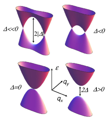
Figure 1: Evolution of the spectrum when the quantity $\Delta$ is varied and changes in sign at the topological transition (arbitrary units). The low-energy spectrum stays linear in the $q_{y}$ direction.

Up to now, we have discussed the merging of the two Dirac points from a “dynamical” point of view, following their motion in the BZ when varying the band parameters until ${\bm{D}}_{0}$ is reached. We now consider the low energy Hamiltonian around ${\bm{D}}_{0}$ even before the two Dirac points coincide. In the neighborhood of the transition when $f({\bm{D}}_{0})=0$, there is a finite gap $2|\Delta|$ at the ${\bm{D}}_{0}$ point (see Fig. 1), where the quantity

$$\Delta=\sum_{mn}(-1)^{\beta_{mn}}t_{mn}$$ (7)

changes its sign at the transition. This parameter $\Delta$ therefore drives the transition. In the vicinity of ${\bm{D}}_{0}$, the Hamiltonian becomes ${\cal H}({\bm{q}})={\cal H}_{0}({\bm{q}})+\Delta\sigma^{x}$, or explicitly :

$${\cal H}({\bm{q}})=\left(\begin{array}[]{cc}0&\Delta+{q_{x}^{2}\over 2m^{*}}-icq_{y}\\ \Delta+{q_{x}^{2}\over 2m^{*}}+icq_{y}&0\\ \end{array}\right)$$ (8)

with the spectrum $\epsilon=\pm\sqrt{(\Delta+q_{x}^{2}/2m^{*})^{2}+c^{2}q_{y}^{2}}$. The Hamiltonian (8) has a remarkable structure and describes properly the vicinity of the topological transition, as shown on Fig. 1. When $m^{*}\Delta$ is negative (we choose $m^{*}>0$ without loss of generality), the spectrum exhibits the two Dirac cones and a saddle point in ${\bm{D}}_{0}$ (at half distance between the two Dirac points). Increasing $\Delta$ from negative to positive values, the saddle point evolves into the hybrid point at the transition ($\Delta=0$) before a gap $2\Delta>0$ opens. Due to the linear spectrum near the Dirac points, the density of states in the semi-metallic phase varies as $|\epsilon|$ at low energy and exhibits a logarithmic divergence $\ln(||\epsilon|-|\Delta||)$ due to the saddle point. At the transition, it varies as $\sqrt{|\epsilon|}$ and then a gap opens for $\Delta>0$ Dietl .

The topological character of the transition is displayed by the cancelation of the Berry phase at the merging of the two Dirac points. The spinorial structure of the wave function leads to a Berry phase ${1\over 2}\oint\nabla\theta_{\bm{q}}\cdot d{\bm{q}}$, where $\theta_{\bm{q}}=\arctan{\mbox{Im}f({\bm{q}})\over\mbox{Re}f({\bm{q}})}$. Near each Dirac point, $\theta_{\bm{q}}=\arctan{q_{y}\over q_{x}}$, whereas $\theta_{\bm{q}}=\arctan{2m^{*}cq_{y}\over q_{x}^{2}}$ near the hybrid ${\bm{D}}_{0}$ point at the transition. Therefore, the Berry phases $\pm\pi$ around each Dirac point annihilate when they merge into ${\bm{D}}_{0}$ Dietl .

We now turn to the evolution of the spectrum in a perpendicular magnetic field $B$. After the substitution $q_{x}\rightarrow q_{x}-eBy$ in the appropriate gauge and the introduction of the dimensionless gap $\delta=\Delta/(m^{*}c^{2}\omega_{c}^{2}/2)^{1/3}$, in terms of the cyclotron frequency $\omega_{c}=eB/m^{*}$, the eigenvalues are $\epsilon_{n}=\pm({\Delta/\delta})\sqrt{E_{n}(\delta)}$ where the $E_{n}$ are solutions of the effective Schrödinger equation

$$E_{n}(\delta)\psi=\big{[}P^{2}+(\delta+Y^{2})^{2}-2Y\big{]}\ \psi\equiv{\cal H}_{eff}\psi$$ (9)

with $[Y,P]=i$. The effective Hamiltonian is therefore of Schrödinger type with a double-well potential when $\delta<0$, which becomes the quartic potential $Y^{4}-2Y$ at the transition and then acquires a gap for $\delta>0$, with a parabolic dispersion at low energy (see Fig. 2). For large negative $\delta$, one recovers two independent parabolic wells with an energy shift $\pm 2\sqrt{\delta}$ equal to half the cyclotron energy. Therefore, as seen in Fig. 2(a), the lowest level has zero energy, and the first levels are degenerate : one recovers the physics of independent Dirac cones in a magnetic field, and the effective energy levels are given by $E_{n}=4n\sqrt{|\delta|}$.

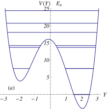
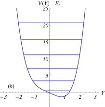
Figure 2: Potential profile $V(Y)=(\delta+Y^{2})^{2}-2Y$ and effective energy levels $E_{n}$ for $\delta=-4$ (a) and $\delta=0$ (b).

Figure 3: Energy levels $\epsilon_{n}(\delta)/(m^{*}c^{2}\omega^{2}/2)^{1/3}$ as a function of the dimensionless parameter $\delta\propto\Delta/B^{2/3}$. The dots on the $\delta=0$ axis indicate the semi-classical levels of the quartic Hamiltonian Dietl .

The complete Landau levels spectrum $\epsilon_{n}(\delta)$ is shown in Fig. 3. The value of the Hall integer is indicated in the gaps between Landau levels. For negative $\delta$, one recovers the spectrum of the Dirac cones, with odd values of the Hall integers – the absence of even values reflects the twofold valley degeneracy of the Landau levels and the presence of a zero-energy Landau level. When $-\delta$ vanishes, approaching the transition, the level degeneracy is lifted, and gaps with even Hall integer open. A simple WKB analysis of the lowest level shows that it splits as $\epsilon_{0}\propto\pm e^{-\#|\delta|^{3/2}}\simeq\pm e^{-\#|\Delta|^{3/2}/B}$. The energy levels scale as $\epsilon_{n}\propto B^{2/3}\sqrt{E_{n}(\Delta/B^{2/3})}$, with the following limits

$$m^{*}\Delta<0\quad,\quad\mbox{semi-metal} \rightarrow \epsilon_{n}\propto\pm\sqrt{nB}$$ (10)

$$\Delta=0\quad,\quad\mbox{transition} \rightarrow \epsilon_{n}\propto\pm[(n+1/2)B]^{2/3}$$

$$m^{*}\Delta>0\quad,\quad\mbox{insulator} \rightarrow \epsilon_{n}=\pm[\Delta+\#(n+1/2)B]$$

Note the shift $n\rightarrow n+1/2$, a consequence of the $\pm\pi$ Berry phases.

We now consider two specific situations in which the merging of Dirac points may be observed. The first example is a variation of the standard graphene tight-binding model, where the three hopping integrals between nearest carbon atoms are assumed to be different:

$$f({\bm{k}})=t_{00}+t_{10}e^{-i{\bm{k}}\cdot{\bm{a}}_{1}}+t_{01}e^{-i{\bm{k}}\cdot{\bm{a}}_{2}}\ .$$ (11)

A merging at ${\bm{D}}_{0}=(p{\bm{a}}_{1}^{*}+q{\bm{a}}_{2}^{*})/2$ is possible if

$$t_{00}+(-1)^{p}t_{10}+(-1)^{q}t_{01}=0\ .$$ (12)

Choosing $t_{00}=t^{\prime}>0$ and $t_{10}=t_{01}=t>0$, Eq. (12) has a solution ($t^{\prime}=2t$) for $p=q=1$, at ${\bm{D}}_{0}=({\bm{a}}_{1}^{*}+{\bm{a}}_{2}^{*})/2$, that is at the $M$ point located at the edge center of the BZ Dietl . Even if the hopping integrals may be modified in graphene under uniaxial stress Goerbig2008 ; CastroNeto2 , it seems impossible to reach physically the merging condition. An alternative for the observation of Dirac points has been proposed with cold atoms in a honeycomb optical lattice. The latter can be realized with laser beams, and by changing the amplitude of the beams, it is possible to vary the band parameters and to reach a situation where the Dirac points merge Zhu .

The organic conductor $\alpha-$(BEDT-TTF)₂I₃ is also a good candidate for the observation of merging Dirac points. In order to study the low-energy spectrum (close to half-filling), the original description with four molecules per unit cell can be reduced to a two-band model in a tetragonal lattice, with the following dispersion relation Hotta ; Katayama2006 ; Kobayashi2007 :

$$f({\bm{k}})=t_{00}+t_{10}e^{i{\bm{k}}\cdot{\bm{a}}_{1}}+t_{01}e^{i{\bm{k}}\cdot{\bm{a}}_{2}}+t_{11}e^{i{\bm{k}}\cdot({\bm{a}}_{1}+{\bm{a}}_{2})}\ .$$ (13)

In this case, the generic spectrum exhibits two Dirac cones the positions of which are given by Goerbig2008

$$\tan^{2}{{\bm{D}}\cdot{\bm{a}}_{1}\over 2}={(t_{00}+t_{01})^{2}-(t_{11}+t_{10})^{2}\over(t_{11}-t_{10})^{2}-(t_{00}-t_{01})^{2}}$$

$$\tan^{2}{{\bm{D}}\cdot{\bm{a}}_{2}\over 2}={(t_{00}+t_{10})^{2}-(t_{11}+t_{01})^{2}\over(t_{11}-t_{01})^{2}-(t_{00}-t_{10})^{2}}\ .$$ (14)

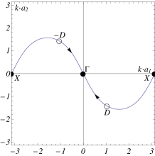
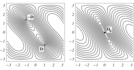
Figure 4: Top figures: left) motion of the two Dirac points ${\bm{D}}$ and $-{\bm{D}}$ for the case $t_{00}=t_{01}=1$, $t_{10}=2+t_{11}$ under variation of $t_{11}$; right) phase diagram. The $\Gamma$ and $X$ lines separate the semi-metallic phase from the band insulator (grey). The Dirac points move from $X=(0,1)$ to the $\Gamma=(0,0)$ point when $t_{11}$ varies from $0$ to $-2$. Bottom figures show the iso-energy curves for $t_{11}=-1.5$ (left) and $-2$ (right).

Upon variation of the band parameters, the two Dirac points may merge when

$$t_{00}+(-1)^{p}t_{10}+(-1)^{q}t_{01}+(-1)^{p+q}t_{11}=0\ .$$ (15)

Katayama et al. have considered the situation (in our notations) where $t_{00}=t_{01}$ Katayama2006 and shown the possibility of a transition from a massless “Dirac” phase to a gapped phase at a hydrostatic pressure $\sim 40$ kbar Kobayashi2007 . In Fig. 4, we show the evolution of the Dirac points in the BZ (as in Ref. Katayama2006 ), and more important, the evolution of the spectrum for a particular variation of the band parameters. The two Dirac points merge at the BZ points $\Gamma$ and $X$ for special values of the band parameters.

The scenario can be even richer. One may imagine a situation where, when varying a band parameter, the Dirac points disappear and then reappear at a different ${\bm{D}}_{0}$ point of the BZ. In Fig. 5, the Dirac points move from $X_{1}$ to $\Gamma$, where a gap opens. For further variation of the band parameter, the gap persists until a new pair of Dirac points appears at a different position $X_{2}$ in the BZ, and disappears again at the fourth special point $X_{3}$.

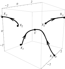
Figure 5: Motion of the Dirac points for model (13), with $t_{00}=-1$, $t_{10}=-0.5$, $t_{01}=1.4$, while varying $-3<t_{11}<3$ (vertical axis).

We finally consider the effect of non-zero diagonal terms in the Hamiltonian (1). When there is inversion symmetry, one has ${\cal H}_{22}({\bm{k}})={\cal H}_{11}(-{\bm{k}})$. Moreover, time-reversal symmetry implies that these diagonal matrix elements are symmetric functions in ${\bm{k}}$, and that their expansion near the hybrid point ${\bm{D}}_{0}={\bm{G}}/2$, has no linear term. Therefore all considerations discussed above remain valid, although the Dirac and hybrid points are no longer necessarily at zero energy.

In conclusion, we have studied under which general conditions the merging of Dirac points may occur, marking the transition between a semi-metal and a band insulator. We have fully described the vicinity of the transition by means of an effective $2\times 2$ Hamiltonian. Although it has been constructed to describe the low energy spectrum near ${\bm{D}}_{0}$, this Hamiltonian is appropriate to describe both valleys around the ${\bm{D}}$ and $-{\bm{D}}$ points avoiding the use of a $4\times 4$ effective Hamiltonian as it is usually done. It may even provide an effective description of graphene, which could be useful, e.g., in accounting for intervalley scattering in a disordered system.

We recently learned of a related work which proposed the existence of hybrid points in the absence of time reversal symmetry in $VO_{2}/TiO_{2}$ heterostructures Pardo2 . We also became aware of a recent independent work on the anisotropic honeycomb lattice in a magnetic field, which has some overlap with ours Esaki . Finally we wish to mention a recent paper on mimicking graphene physics with ultracold fermions in an optical lattice Lee .

Acknowledgments - We acknowledge useful discussions with S. Katayama, A. Kobayashi and T. Nishine.

References

- (1) For a review see A. H. Castro Neto, F. Guinea, N.M.R. Peres, K. Novoselov and A.K. Geim, Rev. Mod. Phys. 81, 109 (2009).
- (2) Y. Hasegawa, R. Konno, H. Nakano and M. Kohmoto, Phys. Rev. B 74, 033413 (2006).
- (3) S.-L. Zhu, B. Wang and L.-M. Duan, Phys. Rev. Lett. 98, 260402 (2007).
- (4) P. Dietl, F. Piéchon and G. Montambaux, Phys. Rev. Lett. 100, 236405 (2008).
- (5) M.O. Goerbig, J.-N. Fuchs, F. Piéchon and G. Montambaux , Phys. Rev. B 78, 045415 (2008).
- (6) V. M. Pereira, A. H. Castro Neto and N. M. R. Peres, Phys. Rev. B 80 045401 (2009)
- (7) B. Wunsch, F. Guinea and F. Sols, New J. Phys. 10, 103027 (2008).
- (8) G.E. Volovik, Lect. Notes Phys. 718, 31 (2007)
- (9) S. Katayama, A. Kobayashi and Y. Suzumura, J. Phys. Soc. Jpn. 75, 054705 (2006).
- (10) A. Kobayashi, S. Katayama, Y. Suzumura and H. Fukuyama, J. Phys. Soc. Jpn. 76, 034711 (2007).
- (11) E. Zhao and A. Paramekanti, Phys. Rev. Lett. 97, 230404 (2006).
- (12) J.-M. Hou, W.-X. Yang and X.-J. Liu, Phys. Rev. A 79, 043621 (2009).
- (13) C. Hotta, J. Phys. Soc. Jpn. 72, 840 (2003).
- (14) S. Banerjee, R.R.P. Singh, V. Pardo and W.E. Pickett, Phys. Rev. Lett. 103, 016402 (2009)
- (15) K. Esaki, M. Sato, M. Kohmoto and B.I. Halperin, Phys. Rev. B 80, 125405 (2009)
- (16) K.L. Lee, B. Grémaud, R. Han, B.-G. Englert and C. Miniatura, arXiv:0906.4158