The inner Cauchy horizon of axisymmetric and stationary black holes with surrounding matter in Einstein-Maxwell theory: study in terms of soliton methods
Abstract
We use soliton methods in order to investigate the interior electrovacuum region of axisymmetric and stationary, electrically charged black holes with arbitrary surrounding matter in Einstein-Maxwell theory. These methods can be applied since the Einstein-Maxwell vacuum equations permit the formulation in terms of the integrability condition of an associated linear matrix problem. We find that there always exists a regular inner Cauchy horizon inside the black hole, provided the angular momentum and charge of the black hole do not vanish simultaneously. Moreover, the soliton methods provide us with an explicit relation for the metric on the inner Cauchy horizon in terms of that on the event horizon. In addition, our analysis reveals the remarkable universal relation , where and denote the areas of event and inner Cauchy horizon respectively.
1 Introduction
The single rotating, electrically charged, axisymmetric and stationary Kerr-Newman black hole in electrovacuum is characterised by the existence of two different so-called Cauchy horizons . One of these horizons is the well-known event horizon which can be considered as a boundary of the exterior electrovacuum world. Outside the event horizon, the Einstein-Maxwell equations take an elliptic form which is related to the fact that in this regime the two Killing vectors and , describing axisymmetry and stationarity respectively, can be combined linearly to form a timelike vector, i.e.111In the formulae (1) and (4) and the corresponding discussion in the text, we exclude points located on the symmetry axis (the ‘rotation axis’). Note that the Killing vector vanishes identically on this axis which implies there.
| (1) |
In contrast, on the event horizon any linear combination of the two Killing vectors is either space-like or null,
| (2) |
i.e. the horizon is a so-called Killing horizon:
| (3) |
where denotes the constant angular velocity of the black hole’s event horizon. This Killing horizon condition leads to specific boundary conditions valid on the event horizon. While in this manner a well-defined elliptic boundary problem of the Einstein-Maxwell equations emerges, it is possible to extend its solution beyond the event horizon into the electrovacuum interior of the black hole. Entering this region, one recognizes that now for the two Killing vectors
| (4) |
holds, meaning that any non-trivial linear combination of the two Killing vectors is space-like. As a consequence, the Einstein-Maxwell vacuum equations are hyberbolic in an inner vicinity of . Taking the boundary values on as ‘initial data’ for this hyperbolic system, one can ‘evolve’ the vacuum solution regularly further into the black hole’s interior. In this manner one finds, for the Kerr-Newman black holes, a ‘future boundary’ of this hyperbolic region, that is the future boundary of the domain of dependence of the event horizon, i.e. the inner Cauchy horizon .
Remarkably, the two horizons of the Kerr-Newman black holes exhibit an interesting relation, which becomes apparent through the equality
| (5) |
where and are angular momentum and charge of the black hole and denote the surface areas of the horizons . Note that for the Kerr-Newman black holes is regular if and only if the left hand side of the above formula is strictly positive, i.e. if and do not vanish simultaneously. Then the black hole singularity is located further inside, that is inside . In the limit the singularity approaches the inner Cauchy horizon, i.e. becomes singular in this limit.
In pure Einsteinian gravity (i.e. without Maxwell field), these observations have been generalized in [2]. It was shown that for axisymmetric and stationary black holes with arbitrary surrounding matter there exists a regular inner Cauchy horizon if and only if holds. Moreover it was possible to identify a general relation between the two horizons through which the metric on is expressed explicitly in terms of that on . As a consequence of this explicit formula it turned out that all such black holes satisfy relation (5) (with ).
It is the aim of this paper to carry this result over to the situation in which electromagnetic fields are included, i.e. to show that for axisymmetric and stationary, electrically charged black holes with arbitrary surrounding matter in Einstein-Maxwell theory
-
1.
there exists a regular inner Cauchy horizon if and only if angular momentum and charge of the black hole do not vanish simultaneously,
-
2.
there is an explicit relation between the metric and electromagnetic quantities on the two horizons ,
-
3.
the universal formula (5) is valid.
Thus, this paper provides a detailed description of the work presented in [9].
For the derivation of the pure Einsteinian results in [2] a particular soliton method was used – the so-called Bäcklund transformation. It was possible to apply this method because the axisymmetric and stationary Einstein vacuum equations can be written in terms of the integrability condition of an associated linear matrix problem. The Bäcklund transformation utilizes this structure and creates a new solution from a previously known one. In [2] this procedure was the essential ingredient in writing an arbitrary regular axisymmetric, stationary black hole solution in terms of another solution, which describes a spacetime without a black hole, but with a completely regular central vacuum region. As a consequence of the symmetries of this regular solution, the desired relation between the two horizons was found.
Proceeding to the Einstein-Maxwell fields, we find that the applicability of the Bäcklund method seems limited. In particular, it is not straightforward to create in this manner the Kerr-Newman solutions from the flat Minkowski space, see [10]. Consequently, in this paper we treat the combined Einstein-Maxwell situation in a different way.
A feature common to both the pure Einstein and the combined Einstein-Maxwell cases is the existence, already mentioned, of an associated linear matrix problem whose integrability condition is equivalent to the field equations in vacuum, see [10]. The Bäcklund transformation is merely one of several solution techniques (another one is the so-called ‘inverse scattering method’, see [14]) whose applicability results from the existence of this linear problem (LP). As will be described below, in the full Einstein-Maxwell situation the integration of the LP along the boundaries of the inner hyperbolic region yields sufficient information to derive the above statements 1–3.
The paper is organized as follows. In Sec. 2, we introduce appropriate coordinates which are adapted to the subsequent analysis. We write the Einstein-Maxwell equations in terms of the Ernst formulation [7] for which the LP can be introduced. Moreover we list necessary horizon boundary and axis regularity conditions. In Sec. 3, we describe the LP and, moreover, show that a similar LP can be found in a rotating frame of reference. The relation of the solution of the LP in the original to that in the rotating frame is derived explicitly. Then, in Sec. 4, we determine the solution of the LP along the boundaries of the inner hyperbolic region, including the two horizons . For this treatment, the known event horizon boundary conditions are taken into account. The derivation of corresponding formulae in the two rotating frames of reference completes the analysis. In this way, an explicit formula relating metric and elctromagnetic potentials on to those on arises, see Sec. 5. As a further consequence of our study of the LP, we show in Sec. 6 the validity of Eq. (5) for axisymmetric and stationary, electrically charged black holes with arbitrary surrounding matter in Einstein-Maxwell theory. Finally, in Sec. 7, we conclude with a discussion.
2 Coordinate systems and Einstein-Maxwell equations
2.1 Weyl coordinates and Boyer-Lindquist-type coordinates
We consider axisymmetric and stationary spacetimes, consisting of an electrically charged central black hole and surrounding matter in Einstein-Maxwell theory. The immediate vicinity of the black hole event horizon must be electrovacuum, see [4] and [3]. In the following, we investigate the metric and electromagnetic potentials in such an electrovacuum region both inside and outside the black hole.
In the exterior electrovacuum vicinity we introduce Weyl coordinates in which the line element reads as follows:
| (6) |
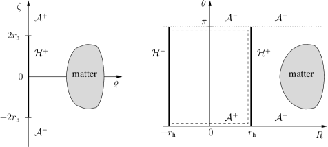
The metric potentials , , and are functions of and alone. As sketched in Fig. 1 (left panel), the event horizon is located on the interval , , of the -axis. The remaining part of the -axis corresponds to the rotation axis. In particular, we denote with and the axis sections where and respectively.
The form (6) of the line element does not characterize uniquely a specific coordinate system. More precisely, if in our ‘original’ system, denoted by , the metric reads as in (6), then in any frame , that rotates at a constant angular velocity with respect to , the line element will assume the same structure. Note that in the coordinates read , with the only new coordinate given by
| (7) |
We will make use of this freedom and choose appropriate coordinate systems and in order to achieve the results of this paper, that is the statements 1–3 in Sec. 1. In particular, we will place ourselves in such an original system in which both the event and inner Cauchy horizon angular velocities do not vanish. More details on this choice are presented in Sec. 3.1.
In order to investigate the interior of the black hole, which is characterized by negative values of , we also introduce Boyer-Lindquist-type coordinates via
| (8) |
(Note that, in the case of the Kerr-Newman black hole, these coordinates are closely related to Boyer-Lindquist coordinates , where the only different coordinate is with denoting the ADM mass of the spacetime.)
In the coordinates , the event horizon is located at . As we shall see below, the inner Cauchy horizon is characterized through , see Fig. 1 (right panel). It is the aim of this paper to show that both metric and electromagnetic quantities are regular in terms of and within the interior vacuum region described by (including ), provided that and do not both vanish.
For convenience, we introduce new metric functions that are, for a regular black hole, analytic in terms of and in the black hole vicinity, see [3],
| (9a) | |||||
| (9b) | |||||
| (9c) | |||||
Moreover, and are strictly positive in that regime. In terms of these functions, the Boyer-Lindquist-type line element is given by
| (10) |
2.2 The Einstein-Maxwell equations
In the electrovacuum region, the electromagnetic field alone constitutes the energy momentum tensor
| (11) |
where is the electromagnetic field tensor. We use the Lorenz gauge, in which can be written in terms of a vector potential ,
| (12) |
Note that, like the metric quantities, and also depend on and only.
We introduce the complex electromagnetic potential and the complex Ernst potential [7, 15] by
| (13) |
where the imaginary parts and are related to metric and vector potentials via
| (14a) | |||||
| (14b) | |||||
| (14c) | |||||
| (14d) | |||||
or, in terms of and ,
| (15a) | |||||
| (15b) | |||||
| (15c) | |||||
| (15d) | |||||
In this formulation, the Einstein-Maxwell equations in electrovacuum are equivalent to the two complex Ernst equations [7]
| (16a) | |||||
| (16b) | |||||
Here, and denote Laplace and nabla operators in flat cylindrical coordinates . In terms of and , these equations take the form
| (17a) | |||
| (17b) | |||
Note that these equations are elliptic for but degenerate at . Only in the interior region are these equations hyperbolic, i.e. in these coordinates the inner Cauchy horizon is a ‘future boundary’ of this hyperbolic vacuum region, that is the future boundary of the domain of dependence of the event horizon , see Fig. 1 (right panel).
2.3 Boundary and regularity conditions
In this section we summarize particular horizon boundary and axis regularity conditions, which are essential in the forthcoming analysis. At the following conditions are satisfied (cf. [3]):
| (18a) | |||
| (18b) | |||
| (18c) |
Here and denote the constant horizon angular velocities and horizon surface gravities respectively, and the comoving electric potential is defined by
| (19) |
As mentioned already, we choose a coordinate frame in which both horizon angular velocities do not vanish (see discussion in Sec. 3.1).
The surface gravities are required to be different from zero, since, in this paper, we exclude degenerate black holes for which and coincide and the hyperbolic region disappears, i.e. we assume .
‘North pole’ and ‘south pole’ of the two horizons are characterized by and respectively. At these points, the horizons meet the rotational axis and the following regularity conditions hold:
| (20) |
The notation and discriminates between the values at north and south pole.
In addition to these conditions, on the portions of the axis , we have
| (21) |
3 The linear problem
The Ernst equations (16) belong to a remarkable class of physically relevant nonlinear partial differential equations, which are characterized by the existence of an associated linear problem (LP) whose integrability conditions are equivalent to the differential equation in question222Other examples of such equations are the Korteweg-de Vries equation, the sine-Gordon equation and the nonlinear Schrödinger equation.. A careful study of this LP will provide us with the information needed to derive the statements 1–3 listed in Sec. 1.
For the formulation of the LP, which is associated with the Ernst equations (16), we introduce the complex coordinates
| (22) |
as well as the function
| (23) |
which depends on the spectral parameter . For fixed values , , equation (23) describes a spectral mapping , from a two-sheeted Riemann surface (-plane) onto the complex -plane. ‘Upper’ and ‘lower’ -sheets (defined by for ) are connected at the two branch points () and ().
The LP is a system of first order differential equations for a matrix pseudopotential , which reads [10]
| (24) |
where
The matrix elements of and are functions of and . In terms of the potentials and they are given by
| (27a) | |||
| (27b) | |||
| (27c) | |||
| (27d) | |||
where can be calculated from and ,
From the integrability condition
of the LP (24) one derives equations that are equivalent to the Ernst equations (16).
The pseudopotential is not uniquely determined by (24). If is a solution, then is also a solution for every matrix function . We can always find a to bring into the form
| (28a) | |||
| and | |||
| (28b) | |||
which depends on three functions , , . Here, the superscript ‘’ or ‘’ indicates whether the functions are evaluated in the upper ( for ) or lower ( for ) sheet of the two-sheeted Riemann -surface. Obviously, of this form is not invertible. Nevertheless, we will see that it still contains sufficient information about and .
3.1 Rotating frames of reference
It turns out that the analysis of the LP, performed alone in the coordinate system with coordinates , does not give sufficient information about the relation of the potentials at the two horizons. However, the missing information can be obtained by studying the situation in the two frames of reference which rotate with the constant horizon angular velocities (cf. (18)) with respect to . Since for the complete investigation needs to be different from , we assume , a choice that can always be made because of the freedom with respect to our original system , see discussion in Sec. 2. Hence, in the formulae appearing below we can safely divide by .
As discussed in Sec. 2, in the coordinate system with coordinates (see (7)) and rotating at the constant angular velocity , the line element possesses again the structure (6). In particular, the corresponding potentials , , and are given in terms of , , and by
| (29a) | |||||
| (29b) | |||||
| (29c) | |||||
The components of the vector potential in the rotating system read
| (30) |
As a consequence, the metric and electromagnetic potentials in again satisfy the Ernst equations (16) (in terms of corresponding potentials and ). Hence an associated LP of the form (24) can be found (with matrices and ). From (14) and (29) it follows that the components of the matrices , read as
| (31a) | |||
| (31b) | |||
| (31c) | |||
| (31d) | |||
with
| (32) |
The pseudopotential in arises as the solution of the LP (24), written in terms of and . It is, however, possible to establish a direct relation between and . As an ansatz, we write
| (33) |
where is an unknown transformation matrix. Combining (24) and the corresponding equations for the LP written in , we conclude that has to obey the equations
| (34a) | |||
| (34b) | |||
A solution, which yields via (33) a pseudopotential that possesses again the special structure (28), turns out to be
| (41) |
Note that this transformation matrix is a generalization of a corresponding expression given in [13, 14] in pure Einsteinian gravity (without Maxwell field).
4 Solution of the linear problem
As we derive in detail below, the relations of the metric and electromagnetic field quantities at the inner Cauchy horizon to those at the event horizon emerge from the integration of the LP along the dashed lines in Fig. 1 (right panel). This integration path contains the parts of the axis as well as the two horizons . We are able to perfom this integration given that and are analytic with respect to and in an exterior vicinity of (including ). Then, and can be expanded into an interior vicinity of . Now, with regular data on a slice inside the black hole, a theorem by Chruściel (theorem 6.3 in [5]333We obtain Chruściels form of the line element by substituting and .) can be applied. Although this theorem is formulated in pure Einsteinian gravity, the arguments presented in [5] permit a generalisation to the Einstein-Maxwell case considered here [6]. The theorem assures that and exist and are regular for all values
i.e. in the entire inner region between the horizons (see Fig. 1), only excluding, for the time being, the inner Cauchy horizon .
Along the entire integration path we have , cf. (8). We study the LP for , that is in the upper sheet of the -plane444With the gauge (28), the solution of the LP in the lower sheet (in which ) can easily be obtained from that in the upper sheet.. Then, the LP reduces to an ODE with the general solution
| (42) |
Here, is a matrix which depends on only. Respecting the gauge (28), the third column of vanishes.
It turns out that the regularity of the potentials and in enables us perform the integration of the LP along and . Moreover, a careful study of the LP for points on the integration path in the vicinities of the north and south poles of reveals that the pseudopotentials possess specific continuity conditions there. In this way it becomes possible to derive the pseudopotentials on and in terms of expressions valid at . Proceeding now to one finds that again the LP exhibits the explicit solution (42) and, most importantly, permits a continuous link of this solution to the pseudopotentials at the two axes sections , which are joined to at the inner Cauchy horizon’s north and south poles. As a result, the regularity of the potentials and at emerges, and their values can be found entirely in terms of those at . This procedure breaks down only if a specific parameter combination (see Eq. (63) below) becomes infinite, which in turn happens if and only if both angular momentum and charge vanish.
We discuss the solutions of the LP on the various sections of the integration path and show that they can be expressed in terms of the three functions and , which are introduced in Sec. 4.1 as ‘integration constants’ of the LP. Moreover, specific north and south pole boundary values of the potentials as well as the constants appear in the integration procedure. In the course of the investigation we find that these values satisfy specific relations. In particular, values at can be written completely in terms of those at . It thus becomes possible to express the inner Cauchy horizon potentials entirely in terms of the event horizon potentials, see Sec. 5.
4.1 Solution on
As expressions valid on become more concise if they are expressed in terms of those at an axis portion that joins the two horizons, we start our considerations of the solution of the LP on .
The gauge (28) does not completely fix the solution of the LP. We obtain a unique solution by imposing the normalization conditions555Note that the conditions (43) are chosen in accordance with regular solvability of the LP along the entire integration path in a complex vicinity of the interval of the real -axis. As in our analysis only values at will be considered, such a vicinity is sufficient, see Sec. 5 and, in particular, Eq. (66).
| (43) |
with
| (44) |
at some point on in the lower sheet of the -plane (). As a consequence of (42), the normalization conditions (43) are then satisfied everywhere on in the lower sheet, and the solution of the LP on in the upper sheet (with ) reads
| (45) |
Here the three ‘integration constants’ , , (depending on ) appear.
4.2 Solution on
On the event horizon, the solution of the LP yields in the upper sheet, i.e. for :
| (53) |
with ‘integration constants’ .
We now derive six equations that provide us with in terms of . These equations follow from the thorough discussion of the LP for points on the integration path in the vicinities of the north and south poles of . In particular, we find that both and (i.e. , , as well as , ) are continuous there. One might expect that the continuity of alone suffices for this investigation, since has, in general, six non-trivial components ( and , , see (28)). However, since at the north and south poles, the LP degenerates there and as a consequence we obtain only two independent equations. Hence, we have to supply this study with further information. We obtain two further independent equations by requiring the continuity of . But as another two equations are needed in order to complete the analysis, we finally consider the continuity of the two expressions and at the north and south poles which again arises as a consequence of the LP. In this manner we gather six independent equations, which allow us to express in terms of :
| (55a) | |||||
| (55b) | |||||
| (55c) | |||||
| (55d) | |||||
| (55e) | |||||
| (55f) | |||||
4.3 Solution on
For the section we write
| (56) |
for the pseudopotential in the upper sheet (). Here
| (57) |
In the rotating system with (cf. Sec. 3.1) we have
| (58) |
As continuity properties valid at the south pole of follow from the LP again, we are able to express the ‘integration constants’ . At first, can be found in terms of . Then, via (55), the arise as functions of , , .
4.4 Solution on
The solution of the LP on is again given by the general structure (42). Hence we may write
| (59) |
for the pseudopotential in the upper sheet () at the inner Cauchy horizon . In the rotating system with (cf. Sec. 3.1) we have
| (60) |
As we cannot assume from the outset that the pseudopotential is regular at and in particular at its north pole, we carefully study whether the LP can be solved on the integration path in the vicinity of this point. We find that this is indeed the case and that, moreover, specific continuity properties can be fulfilled which hold at the pole. These properties are similar to those valid on the poles of , see discussion in Sec. 4.2. As a consequence, the quantities can be derived in terms of , , . Note that the expressions for are of the form (55), with and the superscript ‘’ replaced by and ‘’ respectively.
In a similar manner we may calculate the from continuity conditions studied at the south pole of . Consequently, we obtain two different systems for the , and the requirement of equality of these two sets leads us to the following relations
| (61a) | |||||
| (61b) | |||||
| (61c) | |||||
| (61d) | |||||
| (61e) | |||||
| (61f) | |||||
with
| (62) | |||||
| (63) | |||||
| (64) |
In other words, we are able to express the above boundary values at completely in terms of those on . These relations are essential for expressing the inner Cauchy horizon potentials entirely in terms of the event horizon potentials, see Sec. 5.
5 Ernst potential and electromagnetic potential on the Cauchy horizon
From the pseudopotential , we now calculate the potentials and on . In a first step, we express , , and in terms of the event horizon potentials.
At the branch points and , is unique, i.e. the values in both -sheets coincide. In particular, for (where ) we have
| (66) |
Considering these conditions at , it follows that (cf. (53))
| (67a) | |||
| (67b) | |||
| (67c) | |||
where and are the potentials taken on . Using (55), we obtain a linear system of equations for , , with . The corresponding solution reads
| (68a) | |||||
| (68b) | |||||
| (68c) | |||||
with
| (69) |
Now, we evaluate (66) on . Similarly to (67), we obtain
| (70a) | |||
| (70b) | |||
| (70c) | |||
where and now denote the potentials on . We solve (70) for the two potentials and get
| (71a) | |||||
| (71b) | |||||
Finally, using the expressions for in terms of and Eq. (68), we obtain the potentials on in terms of the potentials on . We arrive at
| (72a) | |||||
| (72b) | |||||
in which the inner Cauchy horizon potentials are given with respect to the Boyer-Lindquist-type coordinate . As before, the superscripts ‘’ and ‘’ indicate quantities on and , respectively. The functions , , , , are given by
where
6 A universal equality
Eqn. (5) contains the following black hole quantities: (i) angular momentum , (ii) electric charge , and (iii) the two horizon surface areas . While the expressions for and are defined unambiguously, the introduction of the angular momentum requires a bit of explanation.
The total angular momentum of the spacetime is composed of matter, electromagnetic field and black hole contributions. While clearly the matter part should be excluded for the definition of the local black hole’s angular momentum, both a Komar integral and an appropriate electromagnetic event horizon integral must be taken into account, in order to find a measure for which Eqn. (5) turns out to be true. A more thorough discussion of this issue is given in [1], at the beginning of Sec. 4, and we here adapt the corresponding expression for the local black hole angular momentum given there.
In terms of the quantities , , and we thus obtain (cf. [1])
| (73a) | |||||
| (73b) | |||||
| (73c) | |||||
where we have used conditions (18) and (20). As in Sec. 1, is the Killing vector with respect to axisymmetry.
In order to show the validity of Eqn. (5), we express at first , , and in terms of the complex potentials and . Using (9), (15), and (19), we can perform the integrations in (73a) and (73b), i.e. we find expressions depending only on values on the north and south poles of the horizons :
| (74a) | |||||
| (74b) | |||||
| (74c) | |||||
where
| (75) |
In order to calculate , we use the solution of the LP on . Evaluation of the conditions in (66), considered on , leads us to
| (76a) | |||||
| (76b) | |||||
| (76c) | |||||
Summming up the first two of these equations we get
| (77) |
With the explicit expression (68a) for , we thus obtain both areas in terms of values on the event horizon’s north pole:
| (78a) | |||||
| (78c) | |||||
Here, we have used that
and
which can be derived from (20) and regularity conditions, that result from the Ernst equations (17), studied at the north and south poles of .
7 Discussion
We have investigated the interior hyperbolic region of axisymmetric and stationary black holes with surrounding matter in Einstein-Maxwell theory. With the help of the LP for the corresponding Ernst equations, we have found the explicit relation (72) for the complex metric and electromagnetic potentials and on the inner Cauchy horizon in terms of those on the event horizon .
A discussion of (72) reveals that with potentials that are regular on , the potentials on are also regular, provided that and do not both vanish. In the limit of vanishing and , the potentials and diverge (cf. the remark at the end of Sec. 4.4).
As an additional result, we have proved a remarkable universal equality for such black holes. Combining our work with a closely related inequality obtained in [8], we arrive at the following.
Theorem 7.1.
Every regular axisymmetric and stationary Einstein-Maxwell black hole with surrounding matter has a regular inner Cauchy horizon if and only if the angular momentum and charge do not both vanish. Then the universal relation
is satisfied where and denote the areas of event and inner Cauchy horizon respectively. If in addition the black hole is sub-extremal (i.e. if there exist trapped surfaces in every sufficiently small interior vicinity of the event horizon), then the following inequalities hold:
Note that in the degenerate limit the above equality becomes identical with the aforementioned inequalities. As indicated in Sec. 2.3, the black hole degenerates if the coordinate radius tends to zero. In this limit the hyperbolic region disappears and the two horizons become identical which in turn means . Then the two formulae in theorem 7.1 yield the known relation for degenerate axisymmetric and stationary black holes with surrounding matter in Einstein-Maxwell theory, see [1].
Acknowledgments
We would like to thank Gernot Neugebauer, Piotr T. Chruściel and David Petroff for many valuable discussions. This work was supported by the Deutsche Forschungsgemeinschaft (DFG) through the Collaborative Research Centre SFB/TR7 ‘Gravitational wave astronomy’.
References
- [1] M. Ansorg and H. Pfister, A universal constraint between charge and rotation rate for degenerate black holes surrounded by matter, Class. Quantum Grav. 25 (2008), 035009.
- [2] M. Ansorg and J. Hennig, The inner Cauchy horizon of axisymmetric and stationary black holes with surrounding matter, Class. Quantum Grav. 25 (2008), 222001.
- [3] J. M. Bardeen, Rapidly rotating stars, disks, and black holes, in Black holes (Les Houches), edited by C. deWitt and B. deWitt (Gordon and Breach, London, 1973), pp. 241-289.
- [4] B. Carter, Black hole equilibrium states in Black Holes (Les Houches), edited by C. deWitt and B. deWitt (Gordon and Breach, London, 1973), pp. 57-214.
- [5] P. T. Chruściel, On space-times with symmetric compact Cauchy surfaces, Ann. Physics 202 (1990), 100.
- [6] P. T. Chruściel, private communication.
- [7] F. J. Ernst, New formulation of the axially symmetric gravitational field problem II, Phys. Rev. 168 (1968), 1415.
- [8] J. Hennig, C. Cederbaum, and M. Ansorg, A universal inequality for axisymmetric and stationary black holes with surrounding matter in the Einstein-Maxwell theory, submitted, arXiv:0812.2811.
- [9] M. Ansorg and J. Hennig, The inner Cauchy horizon of axisymmetric and stationary black holes with surrounding matter in Einstein-Maxwell theory, submitted, arXiv:0903.5405.
- [10] G. Neugebauer and D. Kramer, Einstein-Maxwell solitons, J. Phys. A: Math. Gen. 16 (1983), 1927.
- [11] G. Neugebauer and R. Meinel, General relativistic gravitational field of a rigidly rotating disk of dust: axis potential, disk metric, and surface mass density, Phys. Rev. Lett. 73 (1994), 2166.
- [12] G. Neugebauer and R. Meinel, Phys. Rev. Lett. General relativistic gravitational field of a rigidly rotating disk of dust: solution in terms of ultraelliptic functions, Phys. Rev. Lett. 75 (1995), 3046.
- [13] G. Neugebauer, Rotating bodies as boundary value problems, Ann. Phys. (Leipzig) 9 3-5 (2000), 342.
- [14] G. Neugebauer and R. Meinel, Progress in relativistic gravitational theory using the inverse scattering method, J. Math. Phys. 44 (2003), 3407.
- [15] H. Stephani, D. Kramer, M. MacCallum, C. Hoenselaers, and E. Herlt, Exact solutions of Einstein’s field equations (University Press, Cambridge, 2003).