Quantum spin Hall phases

Abstract

We review our recent theoretical works on the the quantum spin Hall effect. First we compare edge states in various 2D systems, and see whether they are robust or fragile against perturbations. Through the comparisons we see the robust nature of edge states in 2D quantum spin Hall phases. We see how it is protected by the $Z_{2}$ topological number, and reveal the nature of the $Z_{2}$ topological number by studying the phase transition between the quantum spin Hall and insulator phases. We also review our theoretical proposal of the ultrathin bismuth film as a candidate to the 2D quantum spin Hall system.

1 Introduction

Recently spin Hall effect [1, 2] has been studied theoretically and experimentally. It has shed new light onto the physics of the spin-orbit coupling. In the spin Hall effect the spin-orbit coupling plays the role of the spin-dependent effective magnetic field, causing the Hall effect in a spin-dependent way. As a related subject, quantum spin Hall (QSH) phase [3, 4, 5] is recently proposed theoretically. The QSH phase is a novel topological phase, where the bulk is gapped and insulating while there are gapless states localized near the system boundaries. This phase can be found among nonmagnetic insulators, and opened up a renewed interest onto nonmagnetic insulators. This phase is a kind of topological order, and it is not evident compared with other type of orderings such as magnetism and superconductivity. This phase is not an ordered phase in the sense of Ginzburg-Landau theory. It is rather a topological order, which is encoded in the wavefunctions themselves, and it appears only at the boundaries. This topological order is hidden in the bulk, and appears as topologically protected gapless states at the sample boundaries and interfaces. The topological number, in the present case the $Z_{2}$ topological number [3], characterizes whether the system is in the QSH phase or not. In a sense, it plays the role of the “order parameter”. This phase can be realized in 2D and in 3D [6, 7, 8]; the order guarantees the existence of gapless edge states for 2D and gapless surface states for 3D.

The QSH phase resembles the quantum Hall (QH) phase, while there are several important differences. The QSH phase requires an absence of magnetic field, while the QH phase requires a rather strong magnetic field. Moreover, the QH phase is realized usually in 2D, and it is not easily realized in 3D because the motion along the magnetic field usually does not become gapful. In contrast, in the QSH phase there is no such built-in direction and it can be easily realized in 3D as well as in 2D without applying fields.

These gapless edge states in 2D are peculiar in the sense that it is robust against nonmagnetic disorder and interaction [9, 10]. This is in strong constrast with usual states localized at the boundary, which are sensitive to the boundary roughness and impurities and so forth.

Since general readers may not be familiar with this issue, in the first half of this paper we give a general instructive review for the whole subject: “quantum spin Hall phase for pedestrians”. In the latter half we explain our recent research on this topic. The paper is organized as follows. In Section 2 we consider edge states of various 2D systems and see whether they are robust or not. Surface states on the 3D QSH phases is also mentioned. In Section 3 we see how the quantum phase transition between the QSH and insulator phases occurs. Section 4 is devoted to explanations of an existence of gapless helical edge states based on the models obtained in Sec. 3. In Section 5 we theoretically propose that the bismuth ultrathin film will be a good candidate for the 2D QSH phase. In Section 6 we give concluding remarks.

2 Edge States in Various Systems – Fragile or Robust ?

2.1 Edge States in Graphene

Graphene has been studied intensively in recent years. One of the novel properties of graphene is the edge states. It was theoretically proposed by Fujita et al. [11], and was observed by STM experiments. This is a good starting point for studying the edge states in various systems.

One simple way to see the edge states in graphene is the nearest-neighbor tight-binding model on a honeycomb lattice (Fig. 1(a)), described as

$$H=t\sum_{\langle i,j\rangle}c_{i}^{\dagger}c_{j}.$$ (1)

We ignore other details of graphene, since they are inessential to the subsequent discussions. The primitive vectors are

$$\mathbf{a}_{1}=\frac{a}{2}(1,\sqrt{3}),\ \mathbf{a}_{2}=\frac{a}{2}(-1,\sqrt{3}),$$ (2)

and the reciprocal lattice vectors are

$$\mathbf{G}_{1}=\frac{2\pi}{a}\left(1,\frac{1}{\sqrt{3}}\right),\ \mathbf{G}_{2}=\frac{2\pi}{a}\left(-1,\frac{1}{\sqrt{3}}\right).$$ (3)

The Brillouin zone is shown as Fig. 1(b).

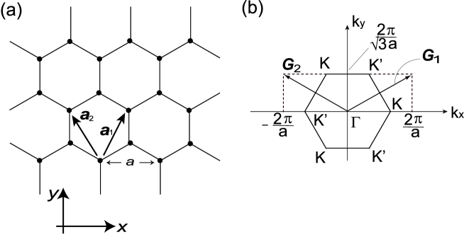
Figure 1: (a) Honeycomb lattice and (b) Brillouin zone corresponding to the honeycomb lattice.

When we consider the tight-binding model on an infinite system, the eigenenergies are

$$E({\bf k})=\pm t\left|e^{i{\bf k}\cdot{\bf a}_{1}}+e^{i{\bf k}\cdot{\bf a}_{2}}+1\right|.$$ (4)

The gap between the valence and the conduction bands closes at two different points in the Brillouin zone, which are called $K$ and $K^{\prime}$ points. Their wavenumbers are

$$\mathbf{k}_{K}=\frac{1}{3}(\mathbf{G}_{1}-\mathbf{G}_{2})=\left(\frac{4\pi}{3a},\ 0\right),\ \mathbf{k}_{K^{\prime}}=-\mathbf{k}_{K}.$$ (5)

Around these points the dispersion is linear and forms Dirac fermions. To study edge states, we consider the system geometry with edges. For this purpose we make the system to have the ribbon geometry, having a finite width in one direction and being infinite in the direction perpendicular to it. The honeycomb lattice allows various types of edge shape, and we choose the zigzag edge and the armchair edge for example. The band structures for the two choices are shown in Fig. 2 (a) and (b), respectively. To understand the obtained band structures in this ribbon geometry, we relate the bulk band structure and that of the ribbon as follows. In the ribbon geometry, the translational symmetry in one direction (perpendicular to the ribbon) is lost and the wavenumber along this direction is no longer a good quantum number. Therefore the bulk band structure is projected along this direction. This almost corresponds to the band structure for the ribbon geometry, calculated in Fig. 2(a) and (b). In the zigzag-edge case (Fig. 2(a)), however, the states located at $E=0$, $\frac{2\pi}{3}<k_{x}a<\frac{4\pi}{3}$ is outside the bulk-band projection. This is nothing but the edge states, because it is located in the bulk band gap, i.e. within the region where the bulk states are prohibited.

Figure 2: Band structure of the nearest-neighbor tight-binding model of the the graphene in the ribbon geometry with (a) zigzag edges and (b) armchair edges.

We note that the above tight-binding model is with drastic simplification. In reality there are many factors which have been ignored here. We thus ask ourselves whether the above properties survive perturbations. For example, within the above tight-binding model, we can introduce various perturbations which do not support edge states. When we vary the boundary conditions, the edge states may vanish. For example, the armchair edge does not support edge states. Another perturbation which kills edge states around $E=0$ is a staggered on-site potential, although it may not be realized in real systems.

This fragility of the edge states arises because the edge states in graphene are not topologically protected, due to vanishing of the bulk gap. In the following sections we see various kinds of robust edge states. All of these robust edge states are associated with respective topological numbers. A more physical reason why the edge states in graphene are fragile is that no current of any kind is flowing along the edge. As we see from Fig. 2(a), the edge states form a flat band, which means that the velocity along the edge is zero. The modes are localized and does not move along the edge. In fact, this flatness of the edge-state band is not a universal property; some perturbations give a dispersion to the otherwise flat band. For example, the next-nearest-neighbor hopping brings about a downward shift of the dispersion around $k_{x}=\pi/a$, compared with Fig. 2 (a). Even in this case, the net current along the edge sums up to zero.

2.2 Edge States in Quantum Hall Systems

In this section we consider an example of robust edge states. We consider the integer QH systems. The QH systems are realized experimentally in a two-dimensional electron system in a strong magnetic field. In the QH systems the bulk is gapped while the edge has gapless edge states, which carries chiral current. The number of chiral edge states, $\nu$, is a topological quantity, which does not change under weak perturbation. In this case the robustness of the edge states comes from the topological number $\nu$. The bulk states bear a topological order, described by the topological number $\nu$ called the Chern number.

The edge states of the QH system look very different from those in the graphene discussed in the previous section. Nevertheless, by using a simple model we can relate them and discuss their differences. It is the model proposed by Haldane [12]. It is a tight-binding model on the honeycomb lattice, where the nearest-neighbor hopping is real, and the next-nearest neighbor hopping is complex. The Hamiltonian is given by

$$H_{{\rm Haldane}}=t_{1}\sum_{\langle i,j\rangle}c_{i}^{\dagger}c_{j}+t_{2}\sum_{\langle\langle i,j\rangle\rangle}e^{-i\nu_{ij}\phi}c_{i}^{\dagger}c_{j}+M\sum_{i}\xi_{i}c_{i}^{\dagger}c_{i}.$$ (6)

Here $\nu_{ij}={\rm sgn}(\hat{{\bf d}}_{1}\times\hat{{\bf d}}_{2})_{z}=\pm 1$, where $\hat{d}_{1}$ and $\hat{d}_{2}$ are unit vectors along the two bonds, which constitute the next-nearest neighbor hopping. $\xi_{i}$ represents a staggered on-site potential, and takes the values $\pm 1$ depending on the $i$-th sites being in the A or B sublattices, respectively. This simply means that the next nearest neighbor hopping, going around the hexagonal plaquette in the clockwise (counterclockwise) way, obtains the phase $e^{i\phi}$ ($e^{-i\phi}$).

The quantization of $\sigma_{xy}$ for this model without impurities can be seen from the Kubo formula, and the resulting $\sigma_{xy}$ is rewritten as $\sigma_{xy}=\nu e^{2}/h$ [13, 14], where

$$\nu=\int_{{\rm BZ}}\sum_{n:{\rm filled}}\frac{d^{2}\bf k}{2\pi}B_{z}^{(n)}({\bf k}),$$ (7)

and

$$B_{z}^{(n)}({\bf k})=\frac{\partial A_{y}^{(n)}({\bf k})}{\partial k_{x}}-\frac{\partial A_{x}^{(n)}({\bf k})}{\partial k_{y}},A_{i}^{(n)}({\bf k})=-i\left\langle u_{n{\bf k}}\right|\frac{\partial}{\partial k_{i}}\left|u_{n{\bf k}}\right\rangle.$$ (8)

The sum in Eq. (7) is taken over the filled bands. The quantity $\nu$ has novel properties arising from topology. A naïve application of the Stokes theorem casts Eq. (7) into a contour integral along the border of the Brillouin zone (BZ), and the periodicity of the BZ results in $\nu=0$; however it is not true [14]. In some cases as the present one, the Bloch wavefunction cannot be expressed as a single continuous function over the whole BZ; the BZ should be divided into pieces, on each of which the Bloch wavefunction is continuous. At the borders between two “pieces” the Bloch wavefunctions differ by a U(1) phase. The number $\nu$ is expressed in terms of this phase difference. As a result one can show that this quantity is quantized to be an integer, and it turns out to be the topological number called the Chern number [13, 14].

This Chern number represents the number of chiral gapless edge states going around the sample edge. Namely the existence of the gapless edge states is guaranteed by the Chern number. This comes from the Laughlin argument [15]; we roll the two-dimensional system into an open cylinder by attaching two edges on the opposite sides, and let a flux $\Phi$ penetrate the hole. The flux $\Phi$ is to be increased from 0 to a flux quantum. Then the number of electrons carried from one edge of the cylinder to the other is equal to the Chern number. These carried electrons are on the gapless edge states. Thus we can establish the correspondence between the number of chiral edge states and the Chern number.

To calculate the value of $\nu$ for the Haldane’s model, it is not easy to calculate Eq.(8) directly, and analytical calculation looks almost impossible. Instead by considering the change of $\nu$ by a change of some parameter, we can easily calculate $\nu$. First we notice that for $\phi=0$ the system is time-reversal symmetric, which yields $\nu=0$, because $\nu$ changes sign under time-reversal. As long as the gap remains open, the Chern number $\nu$ is quantized to be an integer and cannot change when a parameter in the Hamiltonian is continuously changed. In the Haldane’s model, by changing the system parameters, the gap closes only at $K$ and $K^{\prime}$ points. At the gap closing the spectrum of Eq. (6) becomes linear in ${\bf k}$ near the gap-closing point, namely the massless Dirac fermion is formed at the gap closing.

It is straightforward to show the following statement for the change of the Chern number at the gap closing. We consider a $2\times 2$ Hamiltonian matrix $H(M,{\bf k})$, which depends on a parameter $M$. Suppose the gap between the two bands closes at $M=M^{(0)}$ and ${\bf k}={\bf k}^{(0)}$. Then we have $H(M^{(0)},{\bf k}^{(0)})=E_{0}(M^{(0)},{\bf k}^{(0)})\hat{1}$, where $\hat{1}$ is an identity matrix, and we can write

$$H(M,{\bf k})=E_{0}(M,{\bf k})\hat{1}+\sum_{i}a_{i}(M,{\bf k})s_{i},$$ (9)

where $s_{i}$ are Pauli matrices. For notational brevity and convenience we write $k_{0}\equiv M$, $k_{1}=k_{x}$, $k_{2}=k_{y}$. The coefficients $a_{i}$ is expanded in $M$ and ${\bf k}$ in the linear order as

$$a_{i}=\sum_{j=0,1,2}(k_{j}-k_{j}^{(0)})a_{ij}.$$ (10)

Then one can show that the change of the Chern number $\nu$ across $M=M^{(0)}$ is

$$\nu(M=M^{(0)}+\delta)-\nu(M=M^{(0)}-\delta)={\rm sgn}({\rm det}a).$$ (11)

where $a$ is the matrix with elements $a_{ij}$ and $\delta$ is an infinitesimal positive number. Thus the Chern number changes by one at the gap closing. In the present case, the gap closes when $M=\mp 3\sqrt{3}t_{2}\sin\phi$, with ${\bf k}=\pm{\bf k}_{K}=({\bf k}_{K},\ {\bf k}_{K^{\prime}}$), respectively. For the respective cases, the matrix $a$ is calculated by linearlizing the Hamiltonian in the vicinity of the gap closing as

$$a=\left(\begin{array}[]{ccc}1&&\\ &\mp\sqrt{3}a/2&\\ &&-\sqrt{3}a/2\end{array}\right)$$ (12)

and ${\rm sgn}({\rm det}a)=\pm 1$. Thus when we increase $M$ across the value $\mp 3\sqrt{3}t_{2}\sin\phi$, the Chern number increases by $\pm 1$. From this we can easily elaborate the phase diagram as shown in Fig. 3. As we have seen, for analytical calculation it is much easier to calculate the change of the Chern number, than to calculate the Chern number itself.

Figure 3: Phase diagram of the Haldane’s honeycomb-lattice model. $\nu$ represents the Chern number

What is the fundamental differnce between the QH phase and the grephene? The difference comes from the bulk gap. The graphene is gapless while the QH phase has a bulk gap. The topological number in the QH phase protects the existence of the gapless edge states.

2.3 Edge States in 2D Quantum Spin Hall Systems

The QSH system is insulating in the bulk, while there are gapless edge states carrying a spin current. The simplest case of the QSH system is realized by superposing two QH subsystems with opposite spins [5]. We consider the up-spin subsystem with a QH state ($\sigma_{xy}=e^{2}/h$), and the down-spin subsystem with a QH state ($\sigma_{xy}=-e^{2}/h$). The superposition of these states is the QSH state. The edge states consist of two states with opposite spins and velocities. These states are thus carrying a spin current. To realize this state we need a spin-dependent magnetic field, which can be produced by the spin-orbit coupling. This example is just a superposition of two QH systems with conserved spin $s^{z}$. Nevertheless, in real systems, the spin-orbit coupling does not necessarily conserve $s^{z}$, and the above two QH subsystems are mixed with each other. The next question is what happens when $s^{z}$ is no longer a good quantum number. We consider this question in the following, and we see that the physics coming from topology survives partially.

This phase is realized in the model proposed by Kane and Mele [3, 4]. The model is given as

$$H_{KM}=t\sum_{\langle i,j\rangle}c_{i}^{\dagger}c_{j}+i\lambda_{{\rm SO}}\sum_{\langle\langle i,j\rangle\rangle}\nu_{ij}c_{i}^{\dagger}s_{z}c_{j}+i\lambda_{R}\sum_{\langle i,j\rangle}c_{i}^{\dagger}({\bf s}\times\hat{{\bf d}}_{ij})_{z}c_{j}+\lambda_{v}\sum_{i}\xi_{i}c_{i}^{\dagger}c_{i}.$$ (13)

$\xi_{i}$ represents a staggered on-site potential, taking values $\pm 1$ depending on the sublattice index. $\hat{{\bf d}}_{ij}$ is the unit vector along the nearest neighbor bond from $i$ to $j$. For a special case, if $\lambda_{R}=0$ and $\lambda_{v}=0$, the model conserves $s^{z}$ and it reduces to a superposition of two Haldane models:

$$H_{KM}(\lambda_{R}=0,\lambda_{v}=0)=H^{\uparrow}_{{\rm Haldane}}(\phi=-\pi/2)+H^{\downarrow}_{{\rm Haldane}}(\phi=\pi/2).$$ (14)

For generic cases where $s^{z}$ is not conserved, the key ingredient is the time-reversal symmetry, which gives rise to the Kramers degeneracy between ${\bf k}$ and $-{\bf k}$. In the theory the wavenumbers satisfying ${\bf k}\equiv-{\bf k}$ $({\rm mod}\ {\bf G})$ play an important role. Such momenta are called the time-reversal-invariant momenta (TRIM), and are expressed as ${\bf k}={\bf\Gamma}_{i}$ where ${\bf\Gamma}_{i=(n_{1}n_{2})}=\frac{1}{2}(n_{1}{\bf G}_{1}+n_{2}{\bf G}_{2})$ with $n_{1},n_{2}=0,1$ in 2D [3, 16, 17]. The $Z_{2}$ topological number $\nu$ is defined in the following way [16, 17]. First we define a $(2N)\times(2N)$ matrix $w$, defined as

$$w_{mn}({\bf k})=\langle u_{-{\bf k},m}|\Theta|u_{{\bf k},m}\rangle$$ (15)

where $\Theta$ is the time-reversal operator represented as $\Theta=i\sigma_{y}K$ with $K$ being complex conjugation. $u_{m,\mathbf{k}}$ is the periodic part of the $m$-th Bloch wavefunction lying below $E_{F}$, and $N$ is the number of Kramers pairs below $E_{F}$. This matrix $w({\bf k})$ is unitary at any ${\bf k}$, and is also antisymmetric at ${\bf k}={\bf\Gamma}_{i}$. Then for each TRIM we define an index $\delta_{i}$ as

$$\delta_{i}\equiv\frac{\sqrt{{\rm det}w({\bf\Gamma}_{i})}}{{\rm Pf}w({\bf\Gamma}_{i})}.$$ (16)

for ${\cal I}$-asymmetric systems [16], and

$$\delta_{i}\equiv\prod_{m=1}^{N}\xi_{2m}({\bf\Gamma}_{i}),$$ (17)

for ${\cal I}$-symmetric systems [17], where $\xi_{2m}({\bf\Gamma}_{i})$ ($=\pm 1$) is the parity eigenvalue of the Kramers pairs at ${\bf\Gamma}_{i}$. The index $\delta_{i}$ takes the values $\pm 1$. The $Z_{2}$ topological number $\nu$ is then defined as

$$(-1)^{\nu}=\prod_{i=1}^{4}\delta_{i},\ \$$ (18)

where the product is taken over the TRIMs ${\bf k}={\bf\Gamma}_{i}$. Hence $(-1)^{\nu}$ takes only two values $\pm 1$, which means there are only two distinct cases $\nu=\mathrm{even}$ and $\nu=\mathrm{odd}$. For simplicity of notations we henceforth call these cases as $\nu=0$ and $\nu=1$. If the resulting value is $\nu=1$ it is the QSH phase, and if it is $\nu=0$ it is the ordinary insulator. The expression of the $Z_{2}$ topological number is different between systems with and without ${\cal I}$-symmetry. This shows a crucial role of the ${\cal I}$-symmetry in the theory of the QSH systems. It is because the ${\cal I}$ symmetry is the only symmetry operation which relates between ${\bf k}$ and $-{\bf k}$.

To illustrate the physics of the $Z_{2}$ topological number, we calculate the band structure for geometries with edges. Let us consider a ribbon geometry, which is finite in one direction and is infinite in the other direction. To see the difference between two phases, QSH and ordinary insulator (I), we take up the sets of the parameter values for the respective phases, employed in Ref. Kane05b. The result is shown in Figs. 4 and 5 for the QSH and I phases, respectively. As we see from Fig. 4, there exist gapless edge states in the QSH phase, irrespective of the geometry. In contrast, for the insulator phase (Fig. 5) there are no gapless edge states. In fact there are edge states, but they do not go across the gap. These edge states may or may not cross the Fermi energy. Even if they cross the Fermi energy, it is not an intrinsic property, and the crossing can disappear by perturbation.

Figure 4: Band structure of the Kane-Mele model in the QSH phase in the ribbon geometry with (a) zigzag edges and (b) armchair edges. The parameters are $\lambda_{v}=0.1t$, $\lambda_{SO}=0.06t$ and $\lambda_{R}=0.05t$.

Figure 5: Band structure of the Kane-Mele model in the I phase in the ribbon geometry with (a) zigzag edges and (b) armchair edges. The parameters are $\lambda_{v}=0.4t$, $\lambda_{SO}=0.06t$ and $\lambda_{R}=0.05t$.

The bulk band-structure is gapped for both the QSH and I phases and looks similar. Namely, the topological order is not evident in the bulk band structure. The existence of the robust edge states is encoded in the bulk wavefunctions. There is a bulk-edge correspondence:

1. $Z_{2}$ topological number is $\nu=1$ ($\nu=0$).

2. there are odd (even) number of Kramers pairs of gapless edge states.

This correspondence can be shown by the argument similar to the well-known Laughlin’s gedanken experiment [15, 16]. Suppose we consider the system on a ribbon, with two opposite ends attached. In one direction the system is periodic while in the other directions there are edges. When we increase the flux penetrating the hole from zero to half of the flux quantum, the change of a certain physical quantity (time-reversal polarization) is zero for $\nu=0$ while it is unity for $\nu=1$ [16]. This means that for $\nu=1$ there is a Kramers pair of gapless edge states while for $\nu=0$ there are no gapless edge states.

2.4 Surface States in 3D Quantum Spin Hall Systems

The analogous phase is also possible in 3D. In this case this phase is an insulator in the bulk and supports gapless surface states carrying spin currents. In this case as well, there is a correspondence between the bulk and the surface. The topology of Fermi “curve” of the surface states is related with the $Z_{2}$ topological numbers for the bulk.

One can see this by the 3D tight-binding model introduced by Fu et al. [6] on a diamond lattice. This model exhibits a transition between QSH and I phases. The model is written as

$$H=t\sum_{\langle ij\rangle}c_{i}^{\dagger}c_{j}+i(8\lambda_{\mathrm{SO}}/a^{2})\sum_{\langle\langle ij\rangle\rangle}c_{i}^{\dagger}\mathbf{s}\cdot(\mathbf{d}_{ij}^{1}\times\mathbf{d}_{ij}^{2})c_{j}.$$ (19)

Here $a$ is the size of the cubic unit cell, $t$ is the nearest-neighbor hopping, and ${\bf s}=(s_{x},s_{y},s_{z})$ are the Pauli matrices. The term with $\lambda_{\mathrm{SO}}$ is a spin-dependent hopping to the next nearest neighbor sites, representing the spin-orbit coupling. The vectors $\mathbf{d}_{ij}^{1}$ and $\mathbf{d}_{ij}^{2}$ denote those for the two nearest neighbor bonds involved in the next-nearest-neighbor hopping.

In 3D, the TRIMs are ${\bf\Gamma}_{i=(n_{1}n_{2}n_{3})}=\frac{1}{2}(n_{1}{\bf G}_{1}+n_{2}{\bf G}_{2}+n_{3}{\bf G}_{3})$ with $n_{1},n_{2},n_{3}=0,1$. There are four $Z_{2}$ topological numbers $\nu_{0},\nu_{1},\nu_{2},\nu_{3}$ [7, 6], given by

$$(-1)^{\nu_{0}}=\prod_{i=1}^{8}\delta_{i},\ \ (-1)^{\nu_{k}}=\prod_{n_{k}=1;n_{j\neq k}=0,1}\delta_{i=(n_{1}n_{2}n_{3})}.$$ (20)

Each phase is expressed as $\nu_{0};(\nu_{1}\nu_{2}\nu_{3})$, which distinguishes 16 phases. Because among $\nu_{i}$, $\nu_{0}$ is the only topological number which is robust against disorder, the phases are mainly classified by $\nu_{0}$. When $\nu_{0}$ is odd the phase is called the strong topological insulator (STI), and when $\nu_{0}$ is even it is called the weak topological insulator (WTI). The STI and WTI correspond to the QSH and I phases, respectively. The other indices $\nu_{1}$, $\nu_{2}$, and $\nu_{3}$ are used to distinguish various phases in the STI or WTI phases, and each phase can be associated with a mod 2 reciprocal lattice vector $\mathbf{G}_{\nu_{1}\nu_{2}\nu_{3}}=\nu_{1}\mathbf{b}_{1}+\nu_{2}\mathbf{b}_{2}+\nu_{3}\mathbf{b}_{3}$, as was proposed in Ref. Fu06b. These topological numbers in 3D determine the topology of the surface states for arbitrary crystal surfaces [6]. We note that among the four $Z_{2}$ topological numbers in 3D, only $\nu_{0}$ is robust against nonmagnetic impurities, while the others ($\nu_{k}$ ($k=1,2,3$)) are meaningful only for a relatively clean sample [6].

3 Quantum Phase Transition with a Change of Topological Number

As we have seen in the Haldane’s model on the honeycomb lattice, it is hard to calculate the topological number itself and to capture its physical meaning in an intuitive way. The topological number involves an integral over the whole Brillouin zone, both for the QSH systems and the QH systems.

On the other hand, the “change” of the topological number is more accessible. This is because the change occurs locally in ${\bf k}$ space. As we change an external parameter, the system may undergo a phase transition. It accompanies a closing of a bulk gap at a certain ${\bf k}$, because it is the only way to change the topological number. When an external parameter is changed, in some cases the phase transition occurs, while in other cases it does not, because of the level repulsion.

In the following we consider “generic” gap closing by tuning a single parameter, which we call $m$. We exclude the cases where the gap closing is achieved by tuning more than one parameters. In such cases, the phase transition might be circumvented by some perturbation. In general, energy levels repel each other, thereby the valence and the conduction bands do not touch if the number of tuned parameters is not large enough. The number of tuned parameters to achieve degeneracy, called the codimension, is sensitive to the symmetry and the dimension of the system considered.

We henceforth consider only clean systems without any impurities or disorder. The time-reversal symmetry is assumed. We also assume that the Hamiltonian is generic, and we exclude the Hamiltonians which require fine tuning of parameters. In other words, we exclude the cases which are vanishingly improbable as a real material.

3.1 2D Quantum Hall Systems

For the 2D QH systems, it is simple, and in fact we have already seen the physics of gap closing in the Haldane’s model. We can argue gap closing in generic systems, and it becomes similar to the one already described in Section 2. The Chern number is the total flux of $B_{z}({\bf k})$ inside the Brillouin zone. Therefore, if we roll the Brillouin zone into a torus, the Chern number is nothing but a total monopole charge inside the torus, where a monopole and an antimonopole have charges $+1$ and $-1$, respectively. Each band is associated with the respective Chern number. At the gap closing, the Chern number at the lower band changes by $\pm 1$ and that of the upper band changes by $\mp 1$. This means that a monopole (or an antimonopole) goes out of the Brillouin-zone torus of the upper band, and into the Brillouin-zone torus of the lower band.

Let $m$ denote the parameter which drives the phase transition. In the Haldane’s model the on-site staggered potential $M$ plays the role of the parameter $m$. The feature of the phase transition is further clarified by considering a hyperspace $(m,\ k_{x},k_{y})=(k_{0},\ k_{1},\ k_{2})$, and characterizing the gap closing in terms of the gauge field in $m$-${\bf k}$-space [18, 19]. Suppose the gap closes at an isolated point $\tilde{\bf k}=(m,\mathbf{k})$. Then the involved bands, which we call $\alpha$-th and $\beta$-th bands, have monopoles in $m$-${\bf k}$ space, with their monopole charges are opposite in sign [18, 19]. More precisely, the gauge field $\mathbf{A}_{\alpha}(\tilde{\mathbf{k}})$ and the corresponding field strength $\mathbf{B}_{\alpha}(\tilde{\mathbf{k}})$ for the $\alpha$-th band are defined as

$$\mathbf{A}_{\alpha}(\tilde{\mathbf{k}})=-i\langle\psi_{\alpha}(\tilde{\mathbf{k}})|\nabla_{\tilde{\mathbf{k}}}|\psi_{\alpha}(\tilde{\mathbf{k}})\rangle,$$ (21)

$$\mathbf{B}_{\alpha}(\tilde{\mathbf{k}})=\nabla_{\tilde{\mathbf{k}}}\times\mathbf{A}_{\alpha}(\tilde{\mathbf{k}}).$$ (22)

The corresponding monopole density is defined as

$$\rho_{\alpha}(\tilde{\mathbf{k}})=\frac{1}{2\pi}\nabla_{\tilde{\mathbf{k}}}\cdot\mathbf{B}_{\alpha}(\tilde{\mathbf{k}})$$ (23)

Except for the point where $\alpha$-th band touches with other bands, the monopole density $\rho_{\alpha}(\tilde{\mathbf{k}})$ vanishes identically. At the $\tilde{\bf k}$ point where the $\alpha$-th band touches with another band ($\beta$-th band), the wavefunction cannot be written as a single analytic function around this point, and the wavefunction is to be written with more than one “patches” which are related by gauge transformation [14], as is similar to the vector potential around the Dirac monopole in electromagnetism [20]. This leads to a $\delta$-function singularity of $\rho(\tilde{\mathbf{k}})$ at the band touching; $\rho_{\alpha}(\tilde{\bf k})\sim-\rho_{\beta}(\tilde{\bf k})\sim\pm\delta(\tilde{\bf k}=\tilde{\bf k}_{0})$. As a result the monopole density is written in general as $\rho(\tilde{\mathbf{k}})=\sum_{l}q_{l}\delta(\tilde{\mathbf{k}}-\tilde{\mathbf{k}}_{l})$, where $q_{l}$ is an integer representing a monopole charge. The monopole charge is conserved under a continuous change of the Hamiltonian. The monopoles indicate the value of $(m,\mathbf{k})$ where the gap closes. At the monopole, the Chern number for the band considered changes by $\pm 1$.

As an example, in the Haldane’s model on the honeycomb lattice, the gap closes either at $K$ or at $K^{\prime}$. When the gap closing occurs either at $K$ or at $K^{\prime}$, the Chern number changes by one. Meanwhile, when $M$ is changed while $\phi=0$ is kept, the gap closes simultaneously at $K$ and $K^{\prime}$, and the changes of the Chern number at $K$ and $K^{\prime}$ cancel each other; the Chern number does not change as a result.

3.2 Quantum Spin Hall Phase and Universal Phase Diagram

Because the QSH phase is roughly analogous to a superposition of two QH systems, the phase transition can be studied similarly. The $Z_{2}$ topological number is preserved as long as the gap remains open. Suppose the system goes from the insulator to the QSH phase by changing some parameter of the system. Then the gap should close somewhere in between. Whether or not gap closes as the parameter is varied reflects the topological properties of the system. We investigate the criterion for the occurence of the phase transition in Refs. Murakami07a,Murakami07b,Murakami08a, as we explain in the following. Through this study we can show that the gap-closing physics is equivalent to the physics of the $Z_{2}$ topological number.

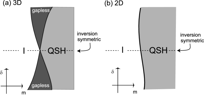
Figure 6: Universal phase diagram between the QSH and the insulator phases in (a) 3D and (b) 2D. $m$ is a parameter driving the phase transition, and $\delta$ is a parameter describing the degree of inversion-symmetry-breaking.

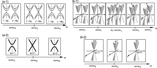
Figure 7: Generic gap-closing for (a-1) 2D inversion-asymmetric, (a-2) 2D inversion-symmetric, (b-1) 3D inversion-asymmetric and (b-2) 3D inversion-symmetric cases. In the cases (a-2) (b-2) all the states are doubly degenerate by Kramers theorem. In (a-1)(a-2) and (b-2), the gap closing and concomitant phase transition occurs only at a single value of $m$: $m=m_{0}$. Meanwhile in (b-1), by increasing $m$, the gap closes at $m=m_{1}$, and the bulk remains gapless in $m_{1}\leq m\leq m_{2}$. The gap opens again at $m=m_{2}$. Although in reality the ${\bf k}$ space is two-dimensional in (a-1)(a-2), and three-dimensional in (b-1)(b-2), it is drawn as one-dimensional in (a-1)(a-2), and two-dimensional in (b-1)(b-2) for clarity of illustration.

To study the phase transition in 2D and in 3D, we consider a Hamiltonian matrix

$$H({\bf k})=\left(\begin{array}[]{cc}h_{\uparrow\uparrow}({\bf k})&h_{\uparrow\downarrow}({\bf k})\\ h_{\downarrow\uparrow}({\bf k})&h_{\downarrow\downarrow}({\bf k})\end{array}\right).$$ (24)

We assume that the system is a band insulator, and the Fermi energy $E_{F}$ lies within the gap. The time-reversal-symmetry gives,

$$H({\bf k})=s_{y}H^{T}(-{\bf k})s_{y},$$ (25)

which is rewritten as $h_{\uparrow\uparrow}({\bf k})=h_{\downarrow\downarrow}^{T}(-{\bf k})$, $h_{\uparrow\downarrow}({\bf k})=-h_{\uparrow\downarrow}^{T}(-{\bf k})$, $h_{\downarrow\uparrow}({\bf k})=-h_{\downarrow\uparrow}^{T}(-{\bf k})$. The Kramers theorem guarantees that the band structure of such time-reversal-symmetric spin-$1/2$ system is symmetric with respect to ${\bf k}\leftrightarrow-{\bf k}$. While the dimension of the Hamiltonian is arbitrary, it will be taken as the number of states involved in the gap closing.

The feature of the phase transition is different whether the system considered is (i) ${\cal I}$-symmetric or (ii) ${\cal I}$-asymmetric [28, 27]. It is because the degeneracy for each state is different for the two cases. According to the Kramers theorem, the time-reversal-symmetry says $\varepsilon_{n\alpha}({\bf k})=\varepsilon_{n{\bar{\alpha}}}(-{\bf k})$, where $\varepsilon_{n\alpha}({\bf k})$ is the energy of the $n$-th band with pseudospin $\alpha$, and ${\bar{\alpha}}$ is the pseudospin opposite to $\alpha$. If in addition, the system is ${\cal I}$-symmetric (i), all the states are doubly degenerate, because the ${\cal I}$-symmetry imposes $\varepsilon_{n\alpha}({\bf k})=\varepsilon_{n\alpha}(-{\bf k})$, leading to $\varepsilon_{n\alpha}({\bf k})=\varepsilon_{n{\bar{\alpha}}}({\bf k})$. If (ii) ${\cal I}$-symmetry is broken, double degeneracy occurs only at points ${\bf k}={\bf\Gamma}_{i}$, where ${\bf\Gamma}_{i}$ is one of the TRIM. By analyzing the respective cases (i)(ii) in 2D and 3D, we obtain a universal phase diagram shown in Fig: 6. Here $m$ is a parameter driving the phase transition, and a parameter $\delta$ describes the degree of inversion-symmetry-breaking. The derivation of this universal phase diagram is generic and based on topological arguments. Hence it does not depend on the details of the system. The parameter $m$ can be any parameter, and in the CdTe/HgTe/CdTe quantum well the well thickness $d$ plays the role of $m$ here.

3.2.1 Inversion asymmetric systems

In ${\cal I}$-asymmetric systems, when ${\bf k}\neq{\bf\Gamma}_{i}$, each band is non-degenerate. At the gap-closing point, one valence band and one conduction band become degenerate. In this case a $2\times 2$ Hamiltonian matrix is sufficient for our purpose;

$$H=\left(\begin{array}[]{cc}a&c\\ c^{*}&b\end{array}\right),$$ (26)

where $a$, $b$ are real functions of ${\bf k}$ and $m$, and $c$ is a complex function of ${\bf k}$ and $m$. A necessary condition for the two eigenvalues to be identical consists of three conditions $a=b$, ${\rm Re}c=0$ and ${\rm Im}c=0$, i.e. the codimension is three [33, 34]. To put it in a different way, the 2$\times$2 Hamiltonian $H(m,\mathbf{k})$ is expanded as

$$H(m,\mathbf{k})=a_{0}(m,\mathbf{k})+\sum_{i=1}^{3}a_{i}(m,\mathbf{k})\sigma_{i}.$$ (27)

The gap closes when the two eigenvalues are identical, i.e. when the three conditions $a_{i}(m,\mathbf{k})$=0 ($i=1,2,3$) are satisfied. This means that the codimension is three.

In 2D, the codimension three is equal to the number of parameters involved, that is, $k_{x}$, $k_{y}$ and $m$. Thus the gap can close at some ${\bf k}$ when the parameter $m$ is tuned to a critical value. Near the gap-closing point ${\bf k}={\bf k}_{0}(\neq{\bf\Gamma}_{i})$, the system’s Hamiltonian corresponds to massive Dirac fermion, and can be expressed as

$${\cal H}=(m-m_{0})\sigma_{z}+(k_{x}-k_{0x})\sigma_{x}+(k_{y}-k_{0y})\sigma_{y}$$ (28)

after unitary and scale transformations. The time-reversal-symmetry requires that the gap closes simultaneously at ${\bf k}_{0}$ and $-{\bf k}_{0}$ as shown in Fig. 7 (a-1), and that the masses of the Dirac fermions at ${\bf k}=\pm{\bf k}_{0}$ have opposite signs. In the Kane-Mele model for the QSH phase [3, 4] the gap closes simultaneously at the $K,K^{\prime}$ points, corresponding to the present case.

In 3D, as is different from 2D, the gap closing at ${\bf k}=\pm{\bf k}_{0}\neq{\bf\Gamma}_{i}$ cannot lead to phase transion. This is because the codimension three is less than the number of parameters $(m,k_{x},k_{y},k_{z})$. The three gap-closing conditions determine a curve in the four-dimensional space $(m,k_{x},k_{y},k_{z})$. When $m$ is changed continuously the gap-closing ${\bf k}$ point moves in the ${\bf k}$ space, and the system remains gapless. This curve forms a loop $C$ in $m$-${\bf k}$ space, and the gap opens when $m$ is changed across the extremum of the loop. The loop $C$ is a trajectory of the gap-closing points i.e. monopoles in the $\mathbf{k}$-space as we change $m$. It forms a closed loop in the $m$-$\mathbf{k}$ space, because of the conservation of the monopole charge. The time-reversal-symmetry requires

$$\mathbf{B}_{\alpha}(\mathbf{k})=-\mathbf{B}_{\bar{\alpha}}(-\mathbf{k}),\ \rho_{\alpha}(\mathbf{k})=\rho_{\bar{\alpha}}(-\mathbf{k}).$$ (29)

The monopoles are symmetric with respect to the origin. Therefore, the generic form of the loop $C$ is as shown in Fig. 8. Thus the loop $C$ occupies a finite region in the value of $m$, and it follows that in ${\cal I}$-asymmetric 3D systems, gapless phase emerges [28], which is nonexistent in 2D.

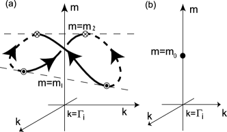
Figure 8: Trajectory of the gap-closing points for (a) inversion- (${\cal I}$-)asymmetric and (b) symmetric systems. For (b) ${\cal I}$-symmetric systems, the gap-closing point is located at $\mathbf{k}={{\bf\Gamma}}_{i}$, and isolated in the $m$-$\mathbf{k}$ space. Only at $m=m_{0}$ the system is gapless. For (a) ${\cal I}$-asymmetric systems, the gap-closing points are created in monopole-antimonopole pairs at $m=m_{1}$, and move in $\mathbf{k}$-space as $m$ changes. Solid and broken curves denote the trajectories of the monopoles and antimonopoles, respectively. The system opens a gap when these gapless points annihilate in pairs at $m=m_{2}$.

So far we discussed the gap closing at ${\bf k}\neq{\bf\Gamma}_{i}$. To complete the discussion, we show that the gap does not close at ${\bf k}={\bf\Gamma}_{i}$, when the system is ${\cal I}$-asymmetric. At ${\bf k}={\bf\Gamma}_{i}$, the band is doubly degenerate, and the codimension is five [35, 36], exceeding the number of tunable parameters which is one (that is, $m$). Thus, generic gap-closing cannot occur at ${\bf k}={\bf\Gamma}_{i}$. One can see this as follows. Because both the valence and the conduction bands are doubly degenerate, we consider $4\times 4$ Hamiltonian matrix with time-reversal-symmetry. From (25) we get

$${H}(m,{\bf k}={\bf\Gamma}_{i})=E_{0}+\sum_{i=1}^{5}a_{i}\Gamma_{i}$$ (30)

where $a_{i}$’s and $E_{0}$ are real, and $\Gamma_{1}=1\otimes\tau_{x}$, $\Gamma_{2}=\sigma_{z}\otimes\tau_{y}$, $\Gamma_{3}=1\otimes\tau_{z}$, $\Gamma_{4}=\sigma_{y}\otimes\tau_{y}$, and $\Gamma_{5}=\sigma_{x}\otimes\tau_{y}$, and $\sigma_{i}$, $\tau_{i}$ are the Pauli matrices. The eigenenergies are $E_{0}\pm\sqrt{\sum_{i=1}^{5}a_{i}^{2}}$. The condition for the gap-closing between the two (doubly-degenerate) bands consists of five equations $a_{i}=0$ for $i=1,\cdots,5$, which are not satisfied by tuning only one parameter $m$. (Here the wavenumber ${\bf k}$ is fixed to be ${\bf\Gamma}_{i}$.) Thus the gap does not close at ${\bf k}={{\bf\Gamma}}_{i}$ by tuning a single parameter $m$.

3.2.2 ${\cal I}$-symmetric systems

In ${\cal I}$-symmetric systems, the energies are doubly degenerate for every ${\bf k}$ by the Kramers theorem. The gap closes between the two doubly-degenerate bands, and we set the Hamiltonian matrix $H({\bf k})$ to be 4$\times$4. The ${\cal I}$-symmetry is imposed as

$$H(-{\bf k})=PH({\bf k})P^{-1},\ u(-{\bf k})=Pu({\bf k}),$$ (31)

where $P$ is a unitary matrix independent of ${\bf k}$ which commutes with the spin matrices, and $u({\bf k})$ is the periodic part of the Bloch wavefunction: $\varphi_{{\bf k}}({r})=u({\bf k})e^{i{\bf k}\cdot{r}}$. Because $P^{2}=1$, the eigenvalues of $P$ are $\pm 1$. By a unitary transformation which diagonalizes $P$, one can rewrite

$$P=\left(\begin{array}[]{cc}P_{\uparrow}&\\ &P_{\downarrow}\end{array}\right),\ \ P_{\uparrow}=P_{\downarrow}={\rm diag}(\eta_{a},\ \eta_{b}),\ \ \eta_{a}=\pm 1,\ \ \eta_{b}=\pm 1$$ (32)

without losing generality. $\eta_{a}$ and $\eta_{b}$ represent the parity eigenvalues of the wavefunctions. One of them corresponds to the valence band, and the other to the conduction band.

While there are four combinations for $\eta_{a}=\pm 1$ and $\eta_{b}=\pm 1$, the overall sign for $(\eta_{a},\eta_{b})$ is arbitrarily changed by gauge transformation. Thus the only distinct case are (i) $\eta_{a}=\eta_{b}$ and (ii) $\eta_{a}=-\eta_{b}$. The case (i) $\eta_{a}=\eta_{b}=\pm 1$ means that the wavefunctions (orbitals) $a$, $b$ have the same parity, e.g. two $s$-like orbitals or two $p$-like orbitals. When $\eta_{a}=\eta_{b}=\pm 1$, the Hamiltonian becomes

$${H}({\bf k})=E_{0}({\bf k})+\sum_{i=1}^{5}a_{i}({\bf k})\Gamma_{i},$$ (33)

where $a_{i}$’s and $E_{0}$ are real even functions of ${\bf k}$. On the other hand, when (ii) $\eta_{a}=-\eta_{b}=\pm 1$, where the two constituent wavefunctions have different parity, the Hamiltonian is

$${H}({\bf k})=E_{0}({\bf k})+a_{5}({\bf k})\Gamma^{\prime}_{5}+\sum_{i=1}^{4}b^{(i)}({\bf k})\Gamma^{\prime}_{i}$$ (34)

where $E_{0}({\bf k})$ and $a_{5}({\bf k})$ are even functions of ${\bf k}$, and $b^{(i)}({\bf k})$ are odd functions of ${\bf k}$. The matrices $\Gamma^{\prime}_{1}=\sigma_{z}\otimes\tau_{x}$, $\Gamma^{\prime}_{2}=1\otimes\tau_{y}$, $\Gamma^{\prime}_{3}=\sigma_{x}\otimes\tau_{x}$, $\Gamma^{\prime}_{4}=\sigma_{y}\otimes\tau_{x}$, and $\Gamma^{\prime}_{5}=1\otimes\tau_{z}$ form the Clifford algebra. Therefore, in both cases, $\eta_{a}=\eta_{b}$ and $\eta_{a}=-\eta_{b}$, the codimension is five, which exceeds the number of tunable parameters ($m$, $k_{x}$, $k_{y}$, $k_{z}$). Therefore, gap closing does not occur in general.

However, this counting holds true only when ${\bf k}$ is at a generic point with ${\bf k}\neq{{\bf\Gamma}}_{i}$, At ${\bf k}={\bf\Gamma}_{i}$, the codimension (number of parameters to achieve degeneracy) remains 5 for $\eta_{a}=\eta_{b}$ (Eq. (33)), while it becomes 1 for $\eta_{a}=-\eta_{b}$ (Eq. (34)). This is because the odd functions $b^{(i)}({\bf k})$ vanish identically at ${\bf k}={\bf\Gamma}_{i}$, and one has only to tune $a_{5}({\bf k})$ to be zero. The number of parameters ($m$) is one, because the wavenumber is fixed as ${\bf k}={{\bf\Gamma}}_{i}$. Thus, the gap closes by fine-tuning a single parameter, only when $\eta_{a}=-\eta_{b}$.

In the following we derive an effective Hamiltonian describing the low-energy physics of the QSH-I phase transition. As a gap-closing point, we take ${\bf k}=0$ as an example, and write down the Hamiltonian explicitly. Extension to other ${\bf k}={\bf\Gamma}_{i}$ points is straightforward. The Hamiltonian is expanded in terms of ${\bf k}$ as

$${H}(m,{\bf k})\sim E_{0}+m\Gamma^{\prime}_{5}+\sum_{i=1}^{4}\left({\bf\beta}^{(i)}\cdot{\bf k}\right)\Gamma^{\prime}_{i},$$ (35)

where $E_{0}$ and $m$ are constants, and ${\bf\beta}^{(i)}$ $(i=1,\cdots,4)$ are two-dimensional real constant vectors. The critical value of $m$ is set as zero. After unitary transformations, the Hamiltonian finally becomes block-diagonal,

$${H}(m,{\bf k})=E_{0}+\left(\begin{array}[]{cccc}m&z_{-}&&\\ z_{+}&-m&&\\ &&m&-z_{+}\\ &&-z_{-}&-m\end{array}\right).$$ (36)

where $z_{\pm}=b_{1}k_{x}+b_{3}k_{y}\pm ib_{2}k_{y}$ with real constants $b_{1}$, $b_{2}$ and $b_{3}$. If the system has fourfold rotational symmetry in the $xy$ plane for example, one has $b_{1}=b_{2}$ and $b_{3}=0$, leading to $z_{\pm}\propto k_{x}\pm ik_{y}$. Thus we have shown that a generic Hamiltonian with time-reversal- and ${\cal I}$- symmetries decouples into a pair of Hamiltonians describing two-component Dirac fermions, with opposite signs of the mass terms. Such decoupling is nontrivial. This Hamiltonian is identical with the one suggested for the HgTe quantum well in Ref. Bernevig06f. The eigenenergies are $E=E_{0}\pm\sqrt{m^{2}+z_{+}z_{-}}$ and the gap closes at ${\bf k}=0$ when the parameter $m$ is tuned to zero. This kind of effective model can be used for studying disorder effects in the QSH phase [30].

3.2.3 $Z_{2}$ Topological Number

We have discussed generic types of gap closing in time-reversal invariant systems, achieved by tuning a single parameter. There are two types of gap closing: (a) simultaneous gap closing at ${\bf k}=\pm{\bf k}_{0}(\neq{\bf\Gamma}_{i})$ occurs in systems without ${\cal I}$-symmetry, and (b) gap closing between two Kramers-degenerate bands (i.e. four bands) at ${\bf k}={\bf\Gamma}_{i}$ occurs in systems with ${\cal I}$-symmetry (see Fig. 7). Thus the gap-closing by tuning a single parameter occurs only in limited cases, due to level repulsion. We note that we have not made any assumption on the $Z_{2}$ topological number, in deriving this result. Nevertheless, we can show that the both cases (a) and (b) involve a change of the $Z_{2}$ topolgical number, and are accompanied by a quantum phase transition. The Kane-Mele model on the honeycomb lattice [4] belongs to class (a) while the HgTe quantum-well model [24] belongs to class (b).

In 2D ${\cal I}$-symmetric systems, the gap closing at the QSH-I transition occurs at TRIM $\mathbf{k}={{\bf\Gamma}}_{i}$. This is accompanied by an exchange of the parity eigenvalues between the valence and the conduction bands. It corresponds to the expression of the $Z_{2}$ topological number as a product of the parity eigenvalues over all the TRIMs $\mathbf{k}={{\bf\Gamma}}_{i}$ over the occupied states [16] (Eq. (17)). On the other hand, for ${\cal I}$-asymmetric 2D systems, the gap closes at $\pm\mathbf{k}_{0}(\neq{\bf\Gamma}_{i})$ by tuning $m$. Because the $Z_{2}$ topological number should change at the gap closing, the $Z_{2}$ topological number should be expressed as an integral over the $\mathbf{k}$ space. This is the Pfaffian expression of the $Z_{2}$ topological number (Eq. (16)) [3, 16]. In retrospect, the gap closing in the ${\cal I}$-symmetric systems occur only at ${\bf\Gamma}_{i}$ between the bands with the opposite parities. This is because otherwise the codimension is five, exceeding the number of tunable parameters. On the other hand, if ${\cal I}$-symmetry is absent, and the level repulsion is less stringent, and the gap can close at some ${\bf k}$ other than the TRIM ${\bf\Gamma}_{i}$. This difference is reflected in the definition of the $Z_{2}$ topological number.

3.3 Example: 3D Fu-Kane-Mele model

The 3D Fu-Kane-Mele model [6] is an ideal model for studying QSH-I phase transitions in 3D. It is a 4-band tight-binding model on a diamond lattice and is ${\cal I}$- and time-reversal-symmetric. It means that every eigenstate is doubly degenerate by the Kramers theorem. The doubly-degenerate conduction band and the valence band touch at the three $X$ points, $X^{r}=(2\pi/a)\hat{r}$ $(r=x,y,z)$. To describe the phases having a bulk gap, one sets the nearest-neighbor hoppings for four bond directions to be different; $t_{i}$ ($i=1,2,3,4$) [6]. The system then opens a gap. When we set the hopping to be $t_{i}=t+\delta t_{i}$ and $\delta t_{3}=0=\delta t_{4}$, the phase diagram is as shown in Fig. 9(a) as a function of $\delta t_{1}$ and $\delta t_{2}$, obtained in Ref. Fu06b. At the phase boundaries the bulk gap vanishes.

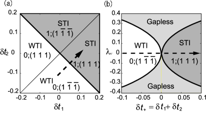
Figure 9: Phase diagrams for the Fu-Kane-Mele model with $\delta t_{3}=0$, $\delta t_{4}=0$. $t_{1}$ and $t_{2}$ are the bonds along the 111 and $1\bar{1}\bar{1}$ directions. We put $\lambda_{\mathrm{SO}}=0.1t$. The axes are in the unit of $t$. (a) The phase diagram in $\delta t_{1}$-$\delta t_{2}$ plane [6]. $\lambda_{v}$ is set as zero. (b) The phase diagram in the $\delta t_{+}$-$\lambda_{v}$ plane. Here $\delta t_{+}=\delta t_{1}+\delta t_{2}$, while $\delta t_{-}=\delta t_{1}-\delta t_{2}=0.1t$ is fixed. The arrows in (a) and (b) refer to the same variation of parameters.

To verify the universal phase diagram in 3D, we introduce the ${\cal I}$-symmetry-breaking term, which does not exist in the original Fu-Kane-Mele model. The simplest way to break ${\cal I}$-symmetry is to introduce an alternating on-site energy $\lambda_{v}$ into the system, as was done the 2D Kane-Mele model on the honeycomb lattice [3].

We then calculate how the WTI-STI phase transition is modified by the $\lambda_{v}$ term. As we see from the phase diagram (Fig. 9(a)) , we regard $\delta t_{+}=\delta t_{1}+\delta t_{2}$ as a parameter $m$ driving the phase transition, while $\delta t_{1}-\delta t_{2}$ is fixed to be $\delta t_{1}-\delta t_{2}=0.1t$ as an example. This corresponds to the arrow in Fig. 9(a). The phase diagram in the $\delta t_{+}$-$\lambda_{v}$ plane is calculated as shown in Fig. 9(b). When the ${\cal I}$-symmetry is broken ($\lambda_{v}\neq 0$), the gapless region appears in the phase diagram, in accordance with our universal phase diagram [29].

The trajectory (“string”) of the gapless points in $\mathbf{k}$ space also agrees with our theory. As the parameter $\delta t_{+}$ is changed along the arrow in Fig. 10(a), the gapless points move in $\mathbf{k}$ space as in Fig. 10(b) [29]. The overall feature of the trajectory, i.e. its pair creation and annihilation with changing partners, perfectly agrees with our theory. The change of the $Z_{2}$ topological numbers is also consistent with our theory [29].

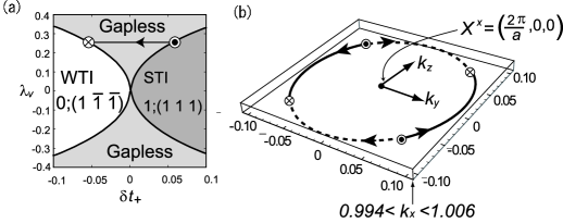
Figure 10: Trajectory of the gapless points in $\mathbf{k}$ space. As we change $\delta t_{+}$ with $\lambda_{v}$ fixed as shown in the arrow in (a), the monopoles and antimonopoles travel in the ${\bf k}$ space as shown in (b) by the solid and broken curves, respectively. The wavenumber $\mathbf{k}$ is shown in the unit of $(2\pi/a)$.

4 Helical edge states

From the effective model thus obtained, we can calculate the helical edge states appearing at the boundary between the QSH and the insulator phase. Such boundary is described by setting the mass parameter $m(x)$ to be dependent on space; $m(\pm\infty)=\pm m_{0}$, i.e.,

$$m=\left\{\begin{array}[]{l}m_{0}\ \ :x\gg 0\\ -m_{0}\ \ :x\ll 0.\end{array}\right.$$ (37)

The detail of the crossover between $m_{0}$ and $-m_{0}$ is unimportant and is left unspecified. For 2D ${\cal I}$-asymmetric systems (Fig. 7(a-1)), one can consider the Dirac fermions at ${\bf k}=\pm{\bf k}_{0}$ separately. Masses of these Dirac fermions change sign at $m=0$; hence they yield the edge states localized at the boundary, as explained in Ref. Niemi86. Because the Dirac fermions at ${\bf k}=\pm{\bf k}_{0}$ are related by time-reversal-reversal symmetry, the two edge states form a Kramers pair and carry a spin current.

For 2D ${\cal I}$-symmetric systems (Fig. 7(a-2)), we follow the discussion in Refs. Niemi86,Su79 to show that such a boundary between phases with different $Z_{2}$ topological numbers has a Kramers pair of edge states. By replacing $k_{x}$ by $-i\partial_{x}$ in Eq. (36), we consider

$$\tilde{H}(k_{y})=E_{0}+b_{1}\partial_{x}\left(\begin{array}[]{cccc}0&-i&&\\ -i&0&&\\ &&0&i\\ &&i&0\end{array}\right)$$ (42)

$$\ \ \ +\left(\begin{array}[]{cccc}m&(b_{3}-ib_{2})k_{y}&&\\ (b_{3}+ib_{2})k_{y}&-m&&\\ &&m&-(b_{3}+ib_{2})k_{y}\\ &&-(b_{3}-ib_{2})k_{y}&-m\end{array}\right).$$ (47)

To calculate the eigenstates it is convenient to perform unitary transformation as

$$H^{\prime}(k_{y})=Q^{\dagger}\tilde{H}({\bf k})Q=E_{0}+\left(\begin{array}[]{cccc}b_{2}k_{y}&m-b_{1}\partial_{x}&&\\ m+b_{1}\partial_{x}&-b_{2}k_{y}&&\\ &&-b_{2}k_{y}&m-b_{1}\partial_{x}\\ &&m+b_{1}\partial_{x}&b_{2}k_{y}\end{array}\right),$$ (48)

where

$$Q=\frac{1}{\sqrt{2}}e^{-ib_{3}k_{y}x/b_{1}}\left(\begin{array}[]{cccc}1&1&&\\ i&-i&&\\ &&-i&-i\\ &&-1&1\end{array}\right).$$ (49)

The eigenvalue problem reads as $H^{\prime}(k_{y})u_{k_{y}}(x)=E(k_{y})u_{k_{y}}(x)$. The term $E_{0}$ is absorbed by shifting the energy. Because (48) is block-diagonal, we first solve the eigenvalue problem for the first two components of $u_{k_{y}}$. By putting $u_{k_{y}}=(u_{1},\ u_{2},\ 0,\ 0)^{t}$, we get

$$(E-b_{2}k_{y})u_{1}=Du_{2},$$ (50)

$$(E+b_{2}k_{y})u_{2}=D^{\dagger}u_{1},$$ (51)

where $D=m-b_{1}\frac{\partial}{\partial x}$, $D^{\dagger}=m+b_{1}\frac{\partial}{\partial x}$. They yield eigenequations for $u_{1}$ and $u_{2}$, respectively:

$$DD^{\dagger}u_{1}=(E^{2}-b_{2}^{2}k_{y}^{2})u_{1},$$ (52)

$$D^{\dagger}Du_{2}=(E^{2}-b_{2}^{2}k_{y}^{2})u_{2}.$$ (53)

Because (52) is invariant under $E\rightarrow-E$, the resulting spectrum seems to be symmetric with respect to $E=0$; $E\leftrightarrow-E$. However, it is not true, because in some cases the $u_{1}$ solutions to (52) has no corresponding solution for $u_{2}$. If $E=-b_{2}k_{y}$, (51) cannot be solved for $u_{2}$. Similarly, if $E=b_{2}k_{y}$, (51) cannot be solved for $u_{1}$. Thus the solutions which are not symmetric with respect to $E=0$ are as follows. For $u_{1}(\neq 0)$ which satisfies $D^{\dagger}u_{1}=0$, we get $E=b_{2}k_{y}$ and $u_{2}=0$ from Eqs. (50) and (51), whereas there is no solution with $E=-b_{2}k_{y}$. In the same token, for $u_{2}$ which satisfies $Du_{2}=0$, we get $E=-b_{2}k_{y}$ from (50), whereas there is no solution with $E=b_{2}k_{y}$. Hence the spectral asymmetry is related to the kernels for $D$ and $D^{\dagger}$. For example, for $b_{1}>0$ and $m_{0}>0$, the solution at the boundary (37), with $D^{\dagger}u_{1}=0$ gives

$$u_{1}\propto\exp\left(-b_{1}^{-1}\int^{x}m(s)ds\right)$$ (54)

and $E=b_{2}k_{y}$, while $Du_{2}=0$ has no normalizable solution. Thus the energy dispersion in $k_{y}$ direction has a branch $E=b_{2}k_{y}$, which crosses the Fermi energy $E\sim 0$. This state is gapless, localized near $x=0$.

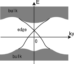
Figure 11: Schematic dispersion curves for the model (47).

We have thus far solved the eigenequation for the first two components. The lower two components of the wavefunction $u$ is obtained from above by time-reversal operation. Therefore, the above-mentioned edge state with $E=b_{2}k_{y}$ has a Kramers partner with $E=-b_{2}k_{y}$. The whole dispersion is shown in Fig. 11. Thus we have shown that the Kramers pair of edge states exists at the boundary between the QSH and I phases. They cross at $k_{y}=0$, as follows from the Kramers theorem.

5 Bismuth Ultrathin Films

The QSH phase requires no magnetic field. This means that some materials might realize the QSH by themselves without applying any field. The only necessary conditions for the QSH systems are as follows.

1. nonmagnetic insulator

2. the $Z_{2}$ topological number is odd ($\nu=1$)

The latter condition means that the spin-orbit coupling should be strong enough, which requires relatively heavier elements. In the absence of the spin-orbit coupling the $Z_{2}$ topological number $\nu$ is zero (i.e. even). When the spin-orbit coupling is made stronger, some systems can change its $Z_{2}$ topological number from $\nu=0$ to $\nu=1$. At the phase transition, the gap closes.

In this sense, the gap should be opened by the spin-orbit coupling. This is an ambiguous statement. In Ref. Murakami06a we clarified that systems with large susceptibility is a good starting point for the materials search. Among materials with heavy elements, we pick up bismuth as a candidate. Bismuth is known as a strong diamagnet, due to interband matrix elements by the spin-orbit coupling. In this sense the gap is originated from the spin-orbit coupling, and is a good candidate for the 2D QSH. Bismuth itself is a nonmagnetic semimetal, not an insulator. We have to open a gap by some means to make it the QSH phase. One idea is to make it into thin film. Indeed, the recent experiments and first-principle calculations show that the (111) 1-bilayer bismuth has indeed a gap [31]. In Ref. Murakami06a we considered the (111) 1-bilayer bismuth ultrathin film from the simple tight-binding model, and theoretically proposed that it is the QSH phase. We also calculate the parity eigenvalues for the tight-binding model, and confirmed the result.

The other way to open a gap is to make an alloy with Sb. This leads us to the 3D QSH, as has been proposed in Ref. Fu06b. In the ARPES measurement [32], the Fermi “surface” for the surface states has been observed, and it crosses the Fermi energy odd times, from the $\bar{\Gamma}$ point to the $\bar{M}$ point. This shows that the surface state of Bi_0.9Sb_0.1 is the topological one for the QSH system.

6 Concluding Remarks

With simple examples we have seen various kinds of edge states. In graphene, the existence of edge states is sensitive to boundary conditions, while in the QH and the QSH systems, the gapless edge states exist irrespective of the boundary conditions. This comes from the nontrivial topological number carried by the bulk states, defined only for insulators. On the other hand, the graphene, being a zero-gap semiconductor, cannot have such topological numbers, which means that the edge states are not robust against perturbations.

The quantum phase transition between the QSH and insulator phases is studied. We consider generic time-reversal-invariant system with a gap, and study the condition when the bulk gap closes by tuning a single external parameter. Due to level repulsion, the gap does not always close by tuning a single parameter; instead in many cases, fine tuning of more than one parameters is needed to close the gap. In the ${\cal I}$-symmetric systems, the gap closes only at the TRIM ${\bf k}={\bf\Gamma}_{i}$, between the valence and conduction bands with opposite parities. In the ${\cal I}$-asymmetric systems, on the other hand, the phase transition is different between 2D and 3D. In 2D the gap closes simultaneously at ${\bf k}=\pm{\bf k}_{0}\neq{\bf\Gamma}_{i}$. In 3D there appears a gapless region in the phase diagram between the QSH and the insulator phases. The gap closing points are monopoles and antimonopoles, and they are created and annihilated in pairs, when the system transits from the gapless phase into the phases with a bulk gap (i.e. QSH or insulator phases).

It is interesting to note that in each case with robust gapless edge states, there is an associated current. In the 2D QH phase it is the charge current which the edge states carry. In the 2D QSH phase it is the spin current. There are also other classies of systems which show this kind of stable edge states. One is the superconductor without time-reversal symmetry, for example with gap function $p_{x}+ip_{y}$. In this case the current of Majorana fermion is carried by the edge states, and the edge states are nothing but the surface Andreev bound states. Another case of interest is found among the superconductors/superfluids with time-reversal symmetry. In this case the edge carries a spin current of the Majorana fermion [40].

References

- [1] S. Murakami, N. Nagaosa and S.-C. Zhang, Science 301 (2003), 1348.
- [2] J. Sinova et al., Phys. Rev. Lett. 92 (2004), 126603.
- [3] C. L. Kane and E. J. Mele, Phys. Rev. Lett. 95 (2005), 226801.
- [4] C. L. Kane and E. J. Mele, Phys. Rev. Lett. 95 (2005), 146802.
- [5] B. A. Bernevig and S.-C. Zhang, Phys. Rev. Lett. 96 (2006), 106802.
- [6] L. Fu, C. L. Kane and E. J. Mele, Phys. Rev. Lett. 98 (2007), 106803.
- [7] J. E. Moore and L. Balents, Phys. Rev. B75 (2007), 121306(R).
- [8] R. Roy, cond-mat/0607531.
- [9] C. Wu, B. A. Bernevig and S.-C. Zhang, Phys. Rev. Lett. 96 (2006), 106401.
- [10] C. Xu and J. E. Moore, Phys. Rev. B 73 (2006), 045322.
- [11] M. Fujita, K. Wakabayashi, K. Nakada and K. Kusakabe, J. Phys. Soc. Jpn. 65 (1996), 1920.
- [12] F. D. M. Haldane, Phys. Rev. Lett. 61 (1988), 2015.
- [13] D. J. Thouless, M. Kohmoto, M. P. Nightingale and M. den Nijs, Phys. Rev. Lett. 49 (1982), 405.
- [14] M. Kohmoto, Ann. Phys. 160 (1985), 343.
- [15] R. B. Laughlin, Phys. Rev. B23 (1981), 5632.
- [16] L. Fu and C. L. Kane, Phys. Rev. B 74 (2006), 195312.
- [17] L. Fu and C. L. Kane, Phys. Rev. B 76 (2007), 045302.
- [18] M. V. Berry, Proc. Roy. Soc. London, Ser. A 392 (1984), 45 .
- [19] G. E. Volovik, The Universe in a Helium Droplet, (Oxford University Press, Oxford, 2003).
- [20] T. T. Wu and C. N. Yang, Phys. Rev. D12 (1975), 3845.
- [21] S. Murakami, N. Nagaosa, and S.-C. Zhang, Phys. Rev. Lett. 93 (2004), 156804.
- [22] B. A. Bernevig, T. L. Hughes and S.-C. Zhang, Science 314 (2006), 1757 .
- [23] T. Hirahara, T. Nagao, I. Matsuda, G. Bihlmayer, E. V. Chulkov, Y. M. Koroteev, P. M. Echenique, M. Saito and S. Hasegawa, Phys. Rev. Lett. 97 (2006),146803 .
- [24] B. A. Bernevig, T. L. Hughes, S.-C. Zhang, Science 314 (2006), 1757.
- [25] M. König, S. Wiedmann, C. Brüne, A. Roth, H. Buhmann, L. W. Molenkamp, X.-L. Qi, and S.-C. Zhang, Science 318 (2007), 766.
- [26] S. Murakami, Phys. Rev. Lett. 97 (2006), 236805.
- [27] S. Murakami, S. Iso, Y. Avishai, M. Onoda, and N. Nagaosa, Phys. Rev. B76 (2007), 205304.
- [28] S. Murakami, New J. Phys. 9 (2007), 356; (Corrigendum) ibid. 10 (2008), 029802.
- [29] S. Murakami and S. Kuga, Phys. Rev. B 78, 165313 (2008).
- [30] R. Shindou and S. Murakami, arXiv:0808.1328.
- [31] Yu. M. Koroteev, G. Bihlmayer, E. V. Chulkov, and S. Blügel, Phys. Rev. B 77 (2008), 045428.
- [32] D. Hsieh, D. Qian, L. Wray, Y. Xia, Y. S. Hor, R. J. Cava and M. Z. Hasan, Nature 452 (2008), 970.
- [33] V. J. von Neumann and E. Wigner, Physik. Zeitschr. 30 (1929), 467.
- [34] C. Herring, Phys. Rev. 52, 361; ibid. 52 (1937), 365.
- [35] J. E. Avron, L. Sadun, J. Segert, and B. Simon, Phys. Rev. Lett. 61 (1988), 1329.
- [36] J. E. Avron, L. Sadun, J. Segert, and B. Simon, Commun. Math. Phys. 124 (1989), 595.
- [37] S. Murakami and N. Nagaosa, Phys. Rev. Lett. 90 (2003), 057002.
- [38] A. J. Niemi and G. W. Semenoff, Phys. Rep. 135 (1986), 99.
- [39] W. P. Su, J. R. Schrieffer, and A. J. Heeger, Phys. Rev. Lett. 42 (1979), 1698.
- [40] X.-L. Qi, T. L. Hughes, S. Raghu and S.-C. Zhang, arXiv:0803.3614.