Joint-sparse recovery from multiple measurements

Abstract

The joint-sparse recovery problem aims to recover, from sets of compressed measurements, unknown sparse matrices with nonzero entries restricted to a subset of rows. This is an extension of the single-measurement-vector (SMV) problem widely studied in compressed sensing. We analyze the recovery properties for two types of recovery algorithms. First, we show that recovery using sum-of-norm minimization cannot exceed the uniform recovery rate of sequential SMV using $\ell_{1}$ minimization, and that there are problems that can be solved with one approach but not with the other. Second, we analyze the performance of the ReMBo algorithm [M. Mishali and Y. Eldar, IEEE Trans. Sig. Proc., 56 (2008)] in combination with $\ell_{1}$ minimization, and show how recovery improves as more measurements are taken. From this analysis it follows that having more measurements than number of nonzero rows does not improve the potential theoretical recovery rate.

1 Introduction

A problem of central importance in compressed sensing [1, 10] is the following: given an $m\times n$ matrix $A$, and a measurement vector $b=Ax_{0}$, recover $x_{0}$. When $m<n$, this problem is ill-posed, and it is not generally possible to uniquely recover $x_{0}$ without some prior information. In many important cases, $x_{0}$ is known to be sparse, and it may be appropriate to solve

$$\mathop{\hbox{minimize}}_{x\in\mathbb{R}^{n}}\quad\|x\|_{0}\quad\mathop{\hbox{subject to}}\quad Ax=b,$$ (1.1)

to find the sparsest possible solution. (The $\ell_{0}$-norm $\|\cdot\|_{0}$ of a vector counts the number of nonzero entries.) If $x_{0}$ has fewer than $s/2$ nonzero entries, where $s$ is the number of nonzeros in the sparsest null-vector of $A$, then $x_{0}$ is the unique solution of this optimization problem [12, 19]. The main obstacle of this approach is that it is combinatorial [24], and therefore impractical for all but the smallest problems. To overcome this, Chen et al. [6] introduced basis pursuit:

$$\mathop{\hbox{minimize}}_{x\in\mathbb{R}^{n}}\quad\|x\|_{1}\quad\mathop{\hbox{subject to}}\quad Ax=b.$$ (1.2)

This convex relaxation, based on the $\ell_{1}$-norm $\|x\|_{1}$, can be solved much more efficiently; moreover, under certain conditions [2, 11], it yields the same solution as the $\ell_{0}$ problem (1.1).

A natural extension of the single-measurement-vector (SMV) problem just described is the multiple-measurement-vector (MMV) problem. Instead of a single measurement $b$, we are given a set of $r$ measurements

$$b^{(k)}=Ax_{0}^{(k)},\quad k=1,\ldots,r,$$

in which the vectors $x_{0}^{(k)}$ are jointly sparse—i.e., have nonzero entries at the same locations. Such problems arise in source localization [22], neuromagnetic imaging [8], and equalization of sparse-communication channels [7, 15]. Succinctly, the aim of the MMV problem is to recover $X_{0}$ from observations $B=AX_{0}$, where $B=[b^{(1)},\ b^{(2)},\ldots,\ b^{(r)}]$ is an $m\times r$ matrix, and the $n\times r$ matrix $X_{0}$ is row sparse—i.e., it has nonzero entries in only a small number of rows. The most widely studied approach to the MMV problem is based on solving the convex optimization problem

$$\mathop{\hbox{minimize}}_{X\in\mathbb{R}^{n\times r}}\quad\|X\|_{p,q}\quad\mathop{\hbox{subject to}}\quad AX=B,$$

where the mixed $\ell_{p,q}$ norm of $X$ is defined as

$$\|X\|_{p,q}=\Big{(}\sum_{j=1}^{n}\|X^{{j}{\scalebox{0.6}{$\rightarrow$}}}\|_{q}^{p}\Big{)}^{1/p},$$

and $X^{{j}{\scalebox{0.6}{$\rightarrow$}}}$ is the (column) vector whose entries form the $j$th row of $X$. In particular, Cotter et al. [8] consider $p=2$, $q\leq 1$; Tropp [28, 29] analyzes $p=1$, $q=\infty$; Malioutov et al. [22] and Eldar and Mishali [14] use $p=1$, $q=2$; and Chen and Huo [5] study $p=1$, $q\geq 1$. A different approach is given by Mishali and Eldar [23], who propose the ReMBo algorithm, which reduces MMV to a series of SMV problems.

In this paper we study the sum-of-norms problem and the conditions for uniform recovery of all $X_{0}$ with a fixed row support, and compare this against recovery using $\ell_{1,1}$. We then construct matrices $X_{0}$ that cannot be recovered using $\ell_{1,1}$ but for which $\ell_{1,2}$ does succeed, and vice versa. We then illustrate the individual recovery properties of $\ell_{1,1}$ and $\ell_{1,2}$ with empirical results. We further show how recovery via $\ell_{1,1}$ changes as the number of measurements increases, and propose a boosted-$\ell_{1}$ approach to improve on the $\ell_{1,1}$ approach. This analysis provides the starting point for our study of the recovery properties of ReMBo, based on a geometrical interpretation of this algorithm.

We begin in Section 2 by summarizing existing $\ell_{0}$-$\ell_{1}$ equivalence results, which give conditions under which the solution of the $\ell_{1}$ relaxation (1.2) coincides with the solution of the $\ell_{0}$ problem (1.1). In Section 3 we consider the $\ell_{1,2}$ mixed-norm and sum-of-norms formulations and compare their performance against $\ell_{1,1}$. In Sections 4 and 5 we examine two approaches that are based on sequential application of (1.2).

Notation.

We assume throughout that $A$ is a full-rank matrix in $\mathbb{R}^{m\times n}$, and that $X_{0}$ is an $s$ row-sparse matrix in $\mathbb{R}^{n\times r}$. We follow the convention that all vectors are column vectors. For an arbitrary matrix $M$, its $j$th column is denoted by the column vector $M^{\scalebox{0.6}{$\downarrow$}{j}}$; its $i$th row is the transpose of the column vector $M^{{i}{\scalebox{0.6}{$\rightarrow$}}}$. The $i$th entry of a vector $v$ is denoted by $v_{i}$. We make exceptions for $e_{i}=I^{\scalebox{0.6}{$\downarrow$}{i}}$ and for $x_{0}$ (resp., $X_{0}$), which represents the sparse vector (resp., matrix) we want to recover. When there is no ambiguity we sometimes write $m_{i}$ to denote $M^{\scalebox{0.6}{$\downarrow$}{i}}$. When concatenating vectors into matrices, $[a,b,c]$ denotes horizontal concatenation and $[a;b;c]$ denotes vertical concatenation. When indexing with $\mathcal{I}$, we define the vector $v_{\mathcal{I}}:=[v_{i}]_{i\in\mathcal{I}}$, and the $m\times|\mathcal{I}|$ matrix $A_{\mathcal{I}}:=[A^{\scalebox{0.6}{$\downarrow$}{j}}]_{j\in\mathcal{I}}$. Row or column selection takes precedence over all other operators.

2 Existing results for $\ell_{1}$ recovery

The conditions under which (1.2) gives the sparsest possible solution have been studied by applying a number of different techniques. By far the most popular analytical approach is based on the restricted isometry property, introduced by Candès and Tao [3], which gives sufficient conditions for equivalence. Donoho [9] obtains necessary and sufficient (NS) conditions by analyzing the underlying geometry of (1.2). Several authors [13, 19, 12] characterize the NS-conditions in terms of properties of the kernel of $A$:

$$\textrm{Ker}(A)=\{x\mid Ax=0\}.$$

Fuchs [16] and Tropp [27] express sufficient conditions in terms of the solution of the dual of (1.2):

$$\mathop{\hbox{maximize}}_{y}\quad b^{T}\!y\quad\mathop{\hbox{subject to}}\quad\|A^{T}\!y\|_{\infty}\leq 1.$$ (2.1)

In this paper we are mainly concerned with the geometric and kernel conditions. We use the geometrical interpretation of the problems to get a better understanding, and resort to the null-space properties of $A$ to analyze recovery. To make the discussion more self-contained, we briefly recall some of the relevant results in the next three sections.

2.1 The geometry of $\ell_{1}$ recovery

The set of all points of the unit $\ell_{1}$-ball, $\{x\in\mathbb{R}^{n}\mid\|x\|_{1}\leq 1\}$, can be formed by taking convex combinations of $\pm e_{j}$, the signed columns of the identity matrix. Geometrically this is equivalent to taking the convex hull of these vectors, giving the cross-polytope $\mathcal{C}=\mathrm{conv}\{\pm e_{1},\pm e_{2},\ldots,\pm e_{n}\}$. Likewise, we can look at the linear mapping $x\mapsto Ax$ for all points $x\in\mathcal{C}$, giving the polytope $\mathcal{P}=\{Ax\mid x\in\mathcal{C}\}=A\mathcal{C}$. The faces of $\mathcal{C}$ can be expressed as the convex hull of subsets of vertices, not including pairs that are reflections with respect to the origin (such pairs are sometimes erroneously referred to as antipodal, which is a slightly more general concept [21]). Under linear transformations, each face from the cross-polytope $\mathcal{C}$ either maps to a face on $\mathcal{P}$ or vanishes into the interior of $\mathcal{P}$.

The solution found by (1.2) can be interpreted as follows. Starting with a radius of zero, we slowly “inflate” $\mathcal{P}$ until it first touches $b$. The radius at which this happens corresponds to the $\ell_{1}$-norm of the solution $x^{*}$. The vertices whose convex hull is the face touching $b$ determine the location and sign of the non-zero entries of $x^{*}$, while the position where $b$ touches the face determines their relative weights. Donoho [9] shows that $x_{0}$ can be recovered from $b=Ax_{0}$ using (1.2) if and only if the face of the (scaled) cross-polytope containing $x_{0}$ maps to a face on $\mathcal{P}$. Two direct consequences are that recovery depends only on the sign pattern of $x_{0}$, and that the probability of recovering a random $s$-sparse vector is equal to the ratio of the number of $(s-1)$-faces in $\mathcal{P}$ to the number of $(s-1)$-faces in $\mathcal{C}$. That is, letting $\mathcal{F}_{d}(\mathcal{P})$ denote the collection of all $d$-faces [21] in $\mathcal{P}$, the probability of recovering $x_{0}$ using $\ell_{1}$ is given by

$$P_{\ell_{1}}(A,s)=\frac{|\mathcal{F}_{s-1}(A\mathcal{C})|}{|\mathcal{F}_{s-1}(\mathcal{C})|}.$$

When we need to find the recoverability of vectors restricted to a support $\mathcal{I}$, this probability becomes

$$P_{\ell_{1}}(A,\mathcal{I})=\frac{|\mathcal{F}_{\mathcal{I}}(A\mathcal{C})|}{|\mathcal{F}_{\mathcal{I}}(\mathcal{C})|},$$ (2.2)

where $\mathcal{F}_{\mathcal{I}}(\mathcal{C})=2^{|\mathcal{I}|}$ denotes the number of faces in $\mathcal{C}$ formed by the convex hull of $\{\pm e_{j}\}_{i\in\mathcal{I}}$, and $\mathcal{F}_{\mathcal{I}}(A\mathcal{C})$ is the number of faces on $A\mathcal{C}$ generated by $\{\pm A^{\scalebox{0.6}{$\downarrow$}{j}}\}_{j\in\mathcal{I}}$.

2.2 Null-space properties and $\ell_{1}$ recovery

Equivalence results in terms of null-space properties generally characterize equivalence for the set of all vectors $x$ with a fixed support, which is defined as

$$\textrm{Supp}(x)=\{j\mid x_{j}\neq 0\}.$$

We say that $x$ can be uniformly recovered on $\mathcal{I}\subseteq\{1,\ldots,n\}$ if all $x$ with $\textrm{Supp}(x)\subseteq\mathcal{I}$ can be recovered. The following theorem illustrates conditions for uniform recovery via $\ell_{1}$ on an index set; more general results are given by Gribonval and Nielsen [20].

Theorem 2.1 (Donoho and Elad [12], Gribonval and Nielsen [19]).

Let $A$ be an $m\times n$ matrix and $\mathcal{I}\subseteq\{1,\ldots,n\}$ be a fixed index set. Then all $x_{0}\in\mathbb{R}^{n}$ with $\textrm{Supp}(x_{0})\subseteq\mathcal{I}$ can be uniquely recovered from $b=Ax_{0}$ using basis pursuit (1.2) if and only if for all $z\in\textrm{Ker}(A)\setminus\{0\}$,

$$\sum_{j\in\mathcal{I}}|z_{j}|<\sum_{j\not\in\mathcal{I}}|z_{j}|.$$ (2.3)

That is, the $\ell_{1}$-norm of $z$ on $\mathcal{I}$ is strictly less than the $\ell_{1}$-norm of $z$ on the complement $\mathcal{I}^{c}$.

2.3 Optimality conditions for $\ell_{1}$ recovery

Sufficient conditions for recovery can be derived from the first-order optimality conditions necessary for $x^{*}$ and $y^{*}$ to be solutions of (1.2) and (2.1) respectively. The Karush-Kuhn-Tucker (KKT) conditions are also sufficient in this case because the problems are convex. The Lagrangian function for (1.2) is given by

$$\mathcal{L}(x,y)=\|x\|_{1}-y^{T}\!(Ax-b);$$

the KKT conditions require that

$$Ax=b\text{and}0\in\partial_{x}\mathcal{L}(x,y),$$ (2.4)

where $\partial_{x}\mathcal{L}$ denotes the subdifferential of $\mathcal{L}$ with respect to $x$. The second condition reduces to

$$0\in\mathop{\hbox{\rm sgn}}(x)-A^{T}\!y,$$

where the signum function

$$\mathop{\hbox{\rm sgn}}(\gamma)\in\begin{cases}\mathop{\hbox{\rm sign}}(\gamma)&\hbox{if $\gamma\neq 0$,}\\ [-1,1]&\hbox{otherwise},\end{cases}$$

is applied to each individual component of $x$. It follows that $x^{*}$ is a solution of (1.2) if and only if $Ax^{*}=b$ and there exists an $m$-vector $y$ such that $|a_{j}^{T}\!y|\leq 1$ for $j\not\in\textrm{Supp}(x)$, and $a_{j}^{T}\!y=\mathop{\hbox{\rm sign}}(x_{j}^{*})$ for all $j\in\textrm{Supp}(x)$. Fuchs [16] shows that $x^{*}$ is the unique solution of (1.2) when $[a_{j}]_{j\in\textrm{Supp}(x)}$ is full rank and, in addition, $|a_{j}^{T}\!y|<1$ for all $j\not\in\textrm{Supp}(x)$. When the columns of $A$ are in general position (i.e., no $k+1$ columns of $A$ span the same $k-1$ dimensional hyperplane for $k\leq n$) we can weaken this condition by noting that for such $A$, the solution of (1.2) is always unique, thus making the existence of a $y$ that satisfies (2.4) for $x_{0}$ a necessary and sufficient condition for $\ell_{1}$ to recover $x_{0}$.

3 Recovery using sums-of-row norms

Our analysis of sparse recovery for the MMV problem of recovering $X_{0}$ from $B=AX_{0}$ begins with an extension of Theorem 2.1 to recovery using the convex relaxation

$$\mathop{\hbox{minimize}}_{X}\quad\sum_{j=1}^{n}\|X^{{j}{\scalebox{0.6}{$\rightarrow$}}}\|\quad\mathop{\hbox{subject to}}\quad AX=B;$$ (3.1)

note that the norm within the summation is arbitrary. Define the row support of a matrix as

$$\textrm{Supp}_{\mathrm{row}}(X)=\{j\mid\|X^{{j}{\scalebox{0.6}{$\rightarrow$}}}\|\neq 0\}.$$

With these definitions we have the following result. (A related result is given by Stojnic et al. [26].)

Theorem 3.1.

Let $A$ be an $m\times n$ matrix, $k$ be a positive integer, $\mathcal{I}\subseteq\{1,\ldots,n\}$ be a fixed index set, and let $\|\cdot\|$ denote any vector norm. Then all $X_{0}\in\mathbb{R}^{n\times r}$ with $\textrm{Supp}_{\mathrm{row}}(X_{0})\subseteq\mathcal{I}$ can be uniquely recovered from $B=AX_{0}$ using (3.1) if and only if for all $Z$ with columns $Z^{\scalebox{0.6}{$\downarrow$}{k}}\in\textrm{Ker}(A)\setminus\{0\}$,

$$\sum_{j\in\mathcal{I}}\|Z^{{j}{\scalebox{0.6}{$\rightarrow$}}}\|<\sum_{j\not\in\mathcal{I}}\|Z^{{j}{\scalebox{0.6}{$\rightarrow$}}}\|.$$ (3.2)

Proof.

For the “only if” part, suppose that there is a $Z$ with columns $Z^{\scalebox{0.6}{$\downarrow$}{k}}\in\textrm{Ker}(A)\setminus\{0\}$ such that (3.2) does not hold. Now, choose $X^{{j}{\scalebox{0.6}{$\rightarrow$}}}=Z^{{j}{\scalebox{0.6}{$\rightarrow$}}}$ for all $j\in\mathcal{I}$ and with all remaining rows zero. Set $B=AX$. Next, define $V=X-Z$, and note that $AV=AX-AZ=AX=B$. The construction of $V$ implies that $\sum_{j}\|X^{{j}{\scalebox{0.6}{$\rightarrow$}}}\|\geq\sum_{j}\|V^{{j}{\scalebox{0.6}{$\rightarrow$}}}\|$, and consequently $X$ cannot be the unique solution of (3.1).

Conversely, let $X$ be an arbitrary matrix with $\textrm{Supp}_{\mathrm{row}}(X)\subseteq\mathcal{I}$, and let $B=AX$. To show that $X$ is the unique solution of (3.1) it suffices to show that for any $Z$ with columns $Z^{\scalebox{0.6}{$\downarrow$}{k}}\in\textrm{Ker}(A)\setminus\{0\}$,

$$\sum_{j}\|(X+Z)^{{j}{\scalebox{0.6}{$\rightarrow$}}}\|>\sum_{j}\|X^{{j}{\scalebox{0.6}{$\rightarrow$}}}\|.$$

This is equivalent to

$$\sum_{j\not\in\mathcal{I}}\|Z^{{j}{\scalebox{0.6}{$\rightarrow$}}}\|+\sum_{j\in\mathcal{I}}\|(X+Z)^{{j}{\scalebox{0.6}{$\rightarrow$}}}\|-\sum_{j\in\mathcal{I}}\|X^{{j}{\scalebox{0.6}{$\rightarrow$}}}\|>0.$$

Applying the reverse triangle inequality, $\|a+b\|-\|b\|\geq-\|a\|$, to the summation over $j\in\mathcal{I}$ and reordering exactly gives condition (3.2). ∎

In the special case of the sum of $\ell_{1}$-norms, i.e., $\ell_{1,1}$, summing the norms of the columns is equivalent to summing the norms of the rows. As a result, (3.1) can be written as

$$\mathop{\hbox{minimize}}_{X}\quad\sum_{k=1}^{r}\|X^{\scalebox{0.6}{$\downarrow$}{k}}\|_{1}\quad\mathop{\hbox{subject to}}\quad AX^{\scalebox{0.6}{$\downarrow$}{k}}=B^{\scalebox{0.6}{$\downarrow$}{k}},\quad k=1,\ldots,r.$$

Because this objective is separable, the problem can be decoupled and solved as a series of independent basis pursuit problems, giving one $X^{\scalebox{0.6}{$\downarrow$}{k}}$ for each column $B^{\scalebox{0.6}{$\downarrow$}{k}}$ of $B$. The following result relates recovery using the sum-of-norms formulation (3.1) to $\ell_{1,1}$ recovery.

Theorem 3.2.

Let $A$ be an $m\times n$ matrix, $r$ be a positive integer, $\mathcal{I}\subseteq\{1,\ldots,n\}$ be a fixed index set, and $\|\cdot\|$ denote any vector norm. Then uniform recovery of all $X\in\mathbb{R}^{n\times r}$ with $\textrm{Supp}_{\mathrm{row}}(X)\subseteq\mathcal{I}$ using sums of norms (3.1) implies uniform recovery on $\mathcal{I}$ using $\ell_{1,1}$.

Proof.

For uniform recovery on support $\mathcal{I}$ to hold it follows from Theorem 3.1 that for any matrix $Z$ with columns $Z^{\scalebox{0.6}{$\downarrow$}{k}}\in\textrm{Ker}(A)\setminus\{0\}$, property (3.2) holds. In particular it holds for $Z$ with $Z^{\scalebox{0.6}{$\downarrow$}{k}}={\bar{z\mkern 2.8mu}\mkern-2.8mu}{}$ for all $k$, with ${\bar{z\mkern 2.8mu}\mkern-2.8mu}{}\in\textrm{Ker}(A)\setminus\{0\}$. Note that for these matrices there exist a norm-dependent constant $\gamma$ such that

$$|{\bar{z\mkern 2.8mu}\mkern-2.8mu}{}_{j}|=\gamma\|Z^{{j}{\scalebox{0.6}{$\rightarrow$}}}\|.$$

Since the choice of ${\bar{z\mkern 2.8mu}\mkern-2.8mu}{}$ was arbitrary, it follows from (3.2) that the NS-condition (2.3) for independent recovery of vectors $B^{\scalebox{0.6}{$\downarrow$}{k}}$ using $\ell_{1}$ in Theorem 2.1 is satisfied. Moreover, because $\ell_{1,1}$ is equivalent to independent recovery, we also have uniform recovery on $\mathcal{I}$ using $\ell_{1,1}$. ∎

An implication of Theorem 3.2 is that the use of restricted isometry conditions—or any technique, for that matter—to analyze uniform recovery conditions for the sum-of-norms approach necessarily lead to results that are no stronger than uniform $\ell_{1}$ recovery. (Recall that the $\ell_{1,1}$ and $\ell_{1}$ norms are equivalent).

3.1 Recovery using $\ell_{1,2}$

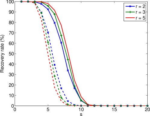
Figure 1: Recovery rates for fixed, randomly drawn $20\times 60$ matrices $A$, averaged over 1,000 trials at each row-sparsity level $s$. The nonzero entries in the $60\times r$ matrix $X_{0}$ are sampled i.i.d. from the normal distribution. The solid and dashed lines represent $\ell_{1,2}$ and $\ell_{1,1}$ recovery, respectively.

In this section we take a closer look at the $\ell_{1,2}$ problem

$$\mathop{\hbox{minimize}}_{X}\quad\|X\|_{1,2}\quad\mathop{\hbox{subject to}}\quad AX=B,$$ (3.3)

which is a special case of the sum-of-norms problem. Although Theorem 3.2 establishes that uniform recovery via $\ell_{1,2}$ is no better than uniform recovery via $\ell_{1,1}$, there are many situations in which it recovers signals that $\ell_{1,1}$ cannot. Indeed, it is evident from Figure 1 that the probability of recovering individual signals with random signs and support is much higher for $\ell_{1,2}$. The reason for the degrading performance or $\ell_{1,1}$ with increasing $k$ is explained in Section 4.

In this section we construct examples for which $\ell_{1,2}$ works and $\ell_{1,1}$ fails, and vice versa. This helps uncover some of the structure of $\ell_{1,2}$, but at the same time implies that certain techniques used to study $\ell_{1}$ can no longer be used directly. Because the examples are based on extensions of the results from Section 2.3, we first develop equivalent conditions here.

3.1.1 Sufficient conditions for recovery via $\ell_{1,2}$

The optimality conditions of the $\ell_{1,2}$ problem (3.3) play a vital role in deriving a set of sufficient conditions for joint-sparse recovery. In this section we derive the dual of (3.3) and the corresponding necessary and sufficient optimality conditions. These allow us to derive sufficient conditions for recovery via $\ell_{1,2}$.

The Lagrangian for (3.3) is defined as

$$\mathcal{L}(X,Y)=\|X\|_{1,2}-\Braket{Y,AX-B},$$ (3.4)

where $\Braket{V,W}\mathrel{\mathop{:}}=\mathop{\hbox{\rm trace}}(V^{T}\!W)$ is an inner-product defined over real matrices. The dual is then given by maximizing

$$\inf_{X}\mathcal{L}(X,Y)=\inf_{X}\left\{\|X\|_{1,2}-\Braket{Y,AX-B}\right\}=\Braket{B,Y}-\sup_{X}\left\{\Braket{A^{T}\!Y,X}-\|X\|_{1,2}\right\}$$ (3.5)

over $Y$. (Because the primal problem has only linear constraints, there necessarily exists a dual solution $Y^{*}$ that maximizes this expression [25, Theorem 28.2].) To simplify the supremum term, we note that for any convex, positively homogeneous function $f$ defined over an inner-product space,

$$\sup_{v}\ \{\Braket{w,v}-f(v)\}=\begin{cases}0&\hbox{if $w\in\partial f(0)$,}\\ \infty&\hbox{otherwise.}\end{cases}$$

To derive these conditions, note that positive homogeneity of $f$ implies that $f(0)=0$, and thus $w\in\partial f(0)$ implies that $\Braket{w,v}\leq f(v)$ for all $v$. Hence, the supremum is achieved with $v=0$. If on the other hand $w\not\in\partial f(0)$, then there exists some $v$ such that $\Braket{w,v}>f(v)$, and by the positive homogeneity of $f$, $\Braket{w,\alpha v}-f(\alpha v)\to\infty$ as $\alpha\to\infty$. Applying this expression for the supremum to (3.5), we arrive at the necessary condition

$$A^{T}\!Y\in\partial\|0\|_{1,2},$$ (3.6)

which is required for dual feasibility.

We now derive an expression for the subdifferential $\partial\|X\|_{1,2}$. For rows $j$ where $\|X^{{j}{\scalebox{0.6}{$\rightarrow$}}}\|_{2}>0$, the gradient is given by $\nabla\|X^{{j}{\scalebox{0.6}{$\rightarrow$}}}\|_{2}=X^{{j}{\scalebox{0.6}{$\rightarrow$}}}/\|X^{{j}{\scalebox{0.6}{$\rightarrow$}}}\|_{2}$. For the remaining rows, the gradient is not defined, but $\partial\|X^{{j}{\scalebox{0.6}{$\rightarrow$}}}\|_{2}$ coincides with the set of unit $\ell_{2}$-norm vectors $\mathcal{B}_{\ell_{2}}^{r}=\{v\in\mathbb{R}^{r}\ \mid\|v\|_{2}\leq 1\}$. Thus, for each $j=1,\ldots,n$,

$$\partial_{X^{{j}{\scalebox{0.6}{$\rightarrow$}}}}\|X\|_{1,2}\in\begin{cases}X^{{j}{\scalebox{0.6}{$\rightarrow$}}}/\|X^{{j}{\scalebox{0.6}{$\rightarrow$}}}\|_{2}&\hbox{if $\|X^{{j}{\scalebox{0.6}{$\rightarrow$}}}\|_{2}>0$,}\\[4.0pt] \mathcal{B}_{\ell_{2}}^{r}&\hbox{otherwise.}\end{cases}$$ (3.7)

Combining this expression with (3.6), we arrive at the dual of (3.3):

$$\mathop{\hbox{maximize}}_{Y}\quad\mathop{\hbox{\rm trace}}(B^{T}\!Y)\quad\mathop{\hbox{subject to}}\quad\|A^{T}\!Y\|_{\infty,2}\leq 1.$$ (3.8)

The following conditions are therefore necessary and sufficient for a primal-dual pair $(X^{*},Y^{*})$ to be optimal for (3.3) and its dual (3.8):

$$AX^{*} =B$$ (primal feasibility); (3.9a)

$$\|A^{T}\!Y^{*}\|_{\infty,2} \leq 1$$ (dual feasibility); (3.9b)

$$\|X^{*}\|_{1,2} =\mathop{\hbox{\rm trace}}(B^{T}\!Y^{*})$$ (zero duality gap). (3.9c)

The existence of a matrix $Y^{*}$ that satisfies (3.9) provides a certificate that the feasible matrix $X^{*}$ is an optimal solution of (3.3). However, it does not guarantee that $X^{*}$ is also the unique solution. The following theorem gives sufficient conditions, similar to those in Section 2.3, that also guarantee uniqueness of the solution.

Theorem 3.3.

Let $A$ be an $m\times n$ matrix, and $B$ be an $m\times r$ matrix. Then a set of sufficient conditions for $X$ to be the unique minimizer of (3.3) with Lagrange multiplier $Y\in\mathbb{R}^{m\times r}$ and row support $\mathcal{I}=\textrm{Supp}_{\mathrm{row}}(X)$, is that

$$AX=B,$$ (3.10a)

$$(A^{T}\!Y)^{\scalebox{0.6}{$\downarrow$}{j}}=(X^{*})^{{j}{\scalebox{0.6}{$\rightarrow$}}}/\|(X^{*})^{{j}{\scalebox{0.6}{$\rightarrow$}}}\|_{2}, \qquad j \in\mathcal{I}$$ (3.10b)

$$\|(A^{T}\!Y)^{\scalebox{0.6}{$\downarrow$}{j}}\|_{2}<1, \qquad j \not\in\mathcal{I}$$ (3.10c)

$$\mathop{\hbox{\rm rank}}(A_{\mathcal{I}})=|\mathcal{I}|.$$ (3.10d)

Proof.

The first three conditions clearly imply that $(X,Y)$ primal and dual feasible, and thus satisfy (3.9a) and (3.9b). Conditions (3.10b) and (3.10c) together imply that

$$\mathop{\hbox{\rm trace}}(B^{T}\!Y)\equiv\sum_{j=1}^{n}[(A^{T}\!Y)^{\scalebox{0.6}{$\downarrow$}{j}}]^{T}X^{{j}{\scalebox{0.6}{$\rightarrow$}}}=\sum_{j=1}^{n}X^{{j}{\scalebox{0.6}{$\rightarrow$}}}\equiv\|X\|_{1,2}.$$

The first and last identities above follow directly from the definitions of the matrix trace and of the norm $\|\cdot\|_{1,2}$, respectively; the middle equality follows from the standard Cauchy inequality. Thus, the zero-gap requirement (3.9c) is satisfied. The conditions (3.10a)–(3.10c) are therefore sufficient for $(X,Y)$ to be an optimal primal-dual solution of (3.3). Because $Y$ determines the support and is a Lagrange multiplier for every solution $X$, this support must be unique. It then follows from condition (3.10d) that $X$ must be unique. ∎

3.2 Counter examples

Using the sufficient and necessary conditions developed in the previous section we now construct examples of problems for which $\ell_{1,2}$ succeeds while $\ell_{1,1}$ fails, and vice versa. Because of its simplicity, we begin with the latter.

Recovery using $\ell_{1,1}$ where $\ell_{1,2}$ fails.

Let $A$ be an $m\times n$ matrix with $m<n$ and unit-norm columns that are not scalar multiples of each other. Take any vector $x\in\mathbb{R}^{n}$ with at least $m+1$ nonzero entries. Then $X_{0}=\mathop{\hbox{\rm diag}}(x)$, possibly with all identically zero columns removed, can be recovered from $B=AX_{0}$ using $\ell_{1,1}$, but not with $\ell_{1,2}$. To see why, note that each column in $X_{0}$ has only a single nonzero entry, and that, under the assumptions on $A$, each one-sparse vector can be recovered individually using $\ell_{1}$ (the points $\pm A^{\scalebox{0.6}{$\downarrow$}{j}}\in\mathbb{R}^{m}$ are all $0$-faces of $\mathcal{P}$) and therefore that $X_{0}$ can be recovered using $\ell_{1,1}$.

On the other hand, for recovery using $\ell_{1,2}$ there would need to exist a matrix $Y$ satisfying the first condition of (3.9) for all $j\in\mathcal{I}=\{1,\ldots,n\}$. For this given $X_{0}$ this reduces to $A^{T}Y=M$, where $M$ is the identity matrix, with the same columns removed as $X$. But this equality is impossible to satisfy because $\mathop{\hbox{\rm rank}}(A)\leq m<m+1\leq\mathop{\hbox{\rm rank}}(M)$. Thus, $X_{0}$ cannot be the solution of the $\ell_{1,2}$ problem (3.3).

Recovery using $\ell_{1,2}$ where $\ell_{1,1}$ fails.

For the construction of a problem where $\ell_{1,2}$ succeeds and $\ell_{1,1}$ fails, we consider two vectors, $f$ and $s$, with the same support $\mathcal{I}$, in such a way that individual $\ell_{1}$ recovery fails for $f$, while it succeeds for $s$. In addition we assume that there exists a vector $y$ that satisfies

$$y^{T}\!A^{\scalebox{0.6}{$\downarrow$}{j}}=\mathop{\hbox{\rm sign}}(s_{j})\quad\hbox{for all $j\in\mathcal{I}$,}\hbox{\qquad and\qquad}|y^{T}\!A^{\scalebox{0.6}{$\downarrow$}{j}}|<1\quad\hbox{for all $j\not\in\mathcal{I}$;}$$

i.e., $y$ satisfies conditions (3.10b) and (3.10c). Using the vectors $f$ and $s$, we construct the 2-column matrix $X_{0}=[(1-\gamma)s,\ \gamma f]$, and claim that for sufficiently small $\gamma>0$, this gives the desired reconstruction problem. Clearly, for any $\gamma\neq 0$, $\ell_{1,1}$ recovery fails because the second column can never be recovered, and we only need to show that $\ell_{1,2}$ does succeed.

For $\gamma=0$, the matrix $Y=[y,0]$ satisfies conditions (3.10b) and (3.10c) and, assuming (3.10d) is also satisfied, $X_{0}$ is the unique solution of $\ell_{1,2}$ with $B=AX_{0}$. For sufficiently small $\gamma>0$, the conditions that $Y$ need to satisfy change slightly due to the division by $\|X_{0}^{{j}{\scalebox{0.6}{$\rightarrow$}}}\|_{2}$ for those rows in $\textrm{Supp}_{\mathrm{row}}(X)$. By adding corrections to the columns of $Y$ those new conditions can be satisfied. In particular, these corrections can be done by adding weighted combinations of the columns in $\bar{Y}$, which are constructed in such a way that it satisfies $A_{\mathcal{I}}^{T}{\bar{Y\mkern 2.0mu}\mkern-2.0mu}{}=I$, and minimizes $\|A_{\mathcal{I}^{c}}^{T}\bar{Y}\|_{\infty,\infty}$ on the complement $\mathcal{I}^{c}$ of $\mathcal{I}$.

Note that on the above argument can also be used to show that $\ell_{1,2}$ fails for $\gamma$ sufficiently close to one. Because the support and signs of $X$ remain the same for all $0<\gamma<1$, we can conclude the following:

Corollary 3.4.

Recovery using $\ell_{1,2}$ is generally not only characterized by the row-support and the sign pattern of the nonzero entries in $X_{0}$, but also by the magnitude of the nonzero entries.

A consequence of this conclusion is that the notion of faces used in the geometrical interpretation of $\ell_{1}$ is not applicable to the $\ell_{1,2}$ problem.

3.3 Experiments

To get an idea of just how much more $\ell_{1,2}$ can recover in the above case where $\ell_{1,1}$ fails, we generated a $20\times 60$ matrix $A$ with entries i.i.d. normally distributed, and determined a set of vectors $s_{i}$ and $f_{i}$ with identical support for which $\ell_{1}$ recovery succeeds and fails, respectively. Using triples of vectors $s_{i}$ and $f_{j}$ we constructed row-sparse matrices such as $X_{0}=[s_{1},f_{1},f_{2}]$ or $X_{0}=[s_{1},s_{2},f_{2}]$, and attempted to recover from $B=AX_{0}W$, where $W=\mathop{\hbox{\rm diag}}(\omega_{1},\omega_{2},\omega_{3})$ is a diagonal weighting matrix with nonnegative entries and unit trace, by solving (3.3). For problems of this size, interior-point methods are very efficient and we use SDPT3 [30] through the CVX interface [18, 17]. We consider $X_{0}$ to be recovered when the maximum absolute difference between $X_{0}$ and the $\ell_{1,2}$ solution $X^{*}$ is less than $10^{-5}$. The results of the experiment are shown in Figure 2. In addition to the expected regions of recovery around individual columns $s_{i}$ and failure around $f_{i}$, we see that certain combinations of vectors $s_{i}$ still fail, while other combinations of vectors $f_{i}$ may be recoverable. By contrast, when using $\ell_{1,1}$ to solve the problem, any combination of $s_{i}$ vectors can be recovered while no combination including an $f_{i}$ can be recovered.

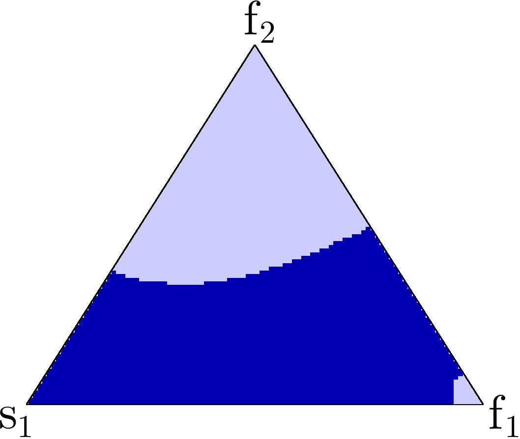
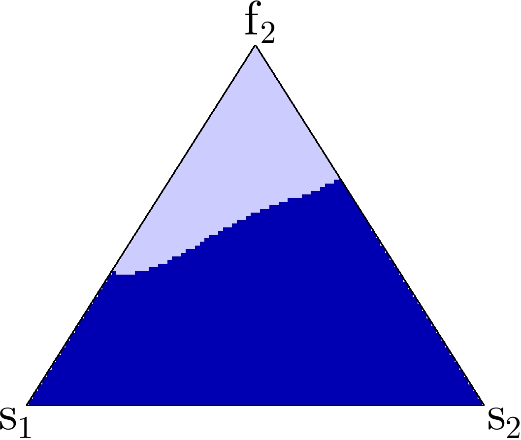
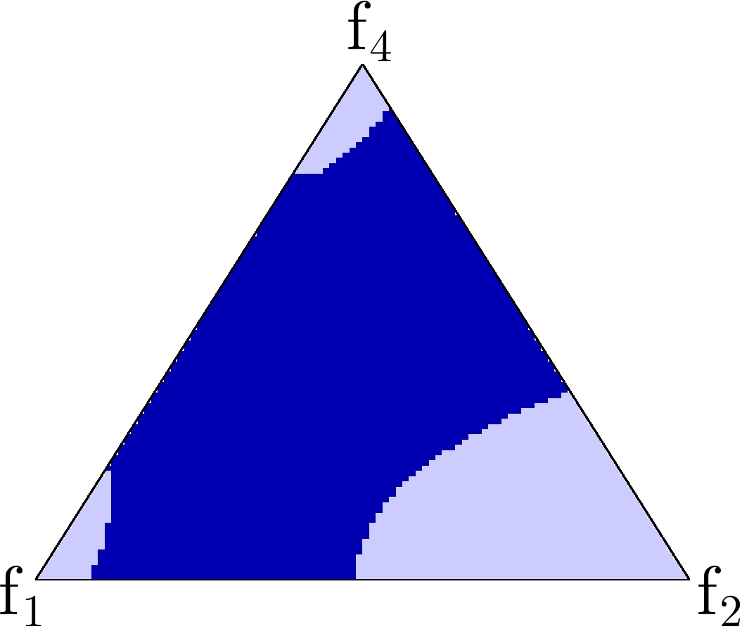
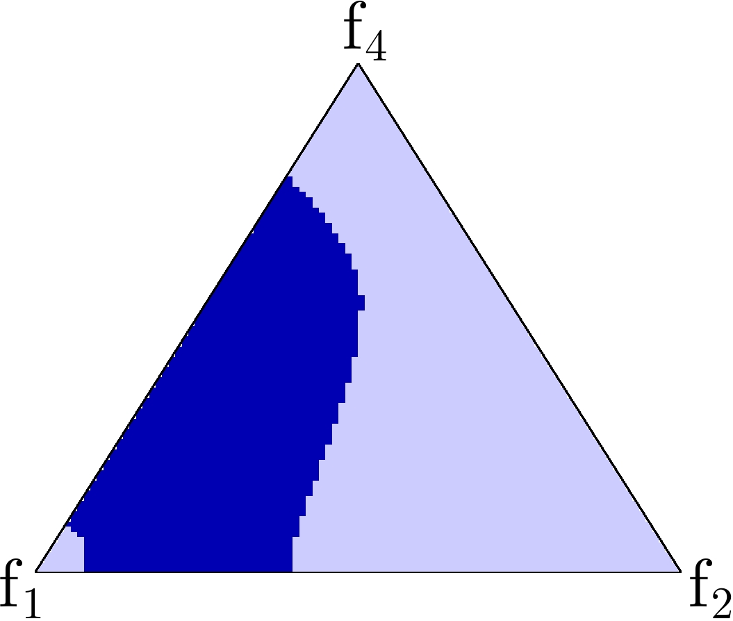
$|\mathcal{I}|=5$	$|\mathcal{I}|=5$	$|\mathcal{I}|=5$	$|\mathcal{I}|=7$
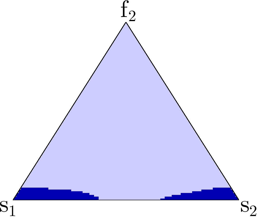
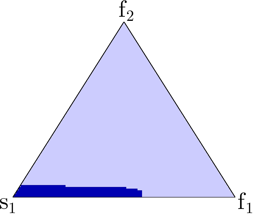
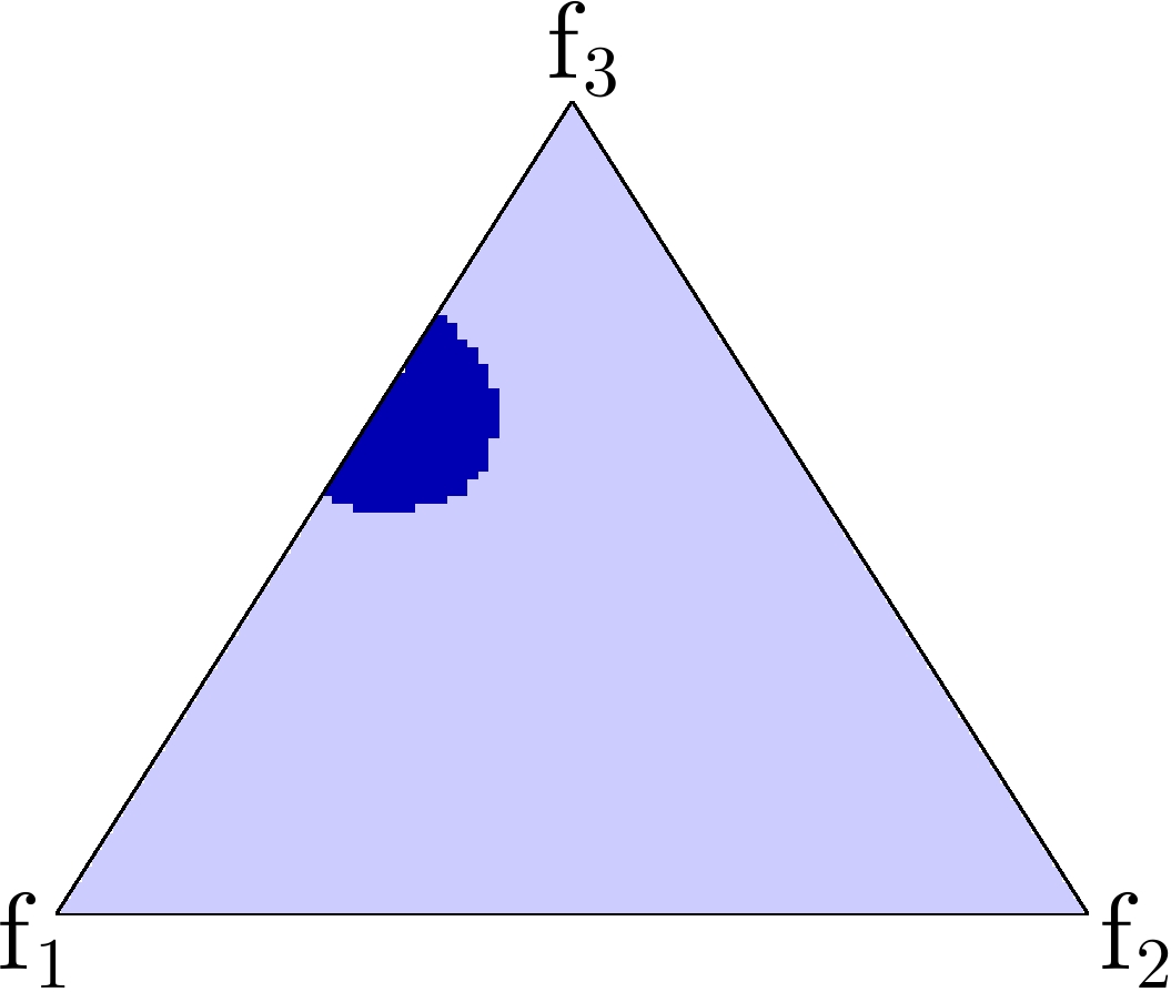
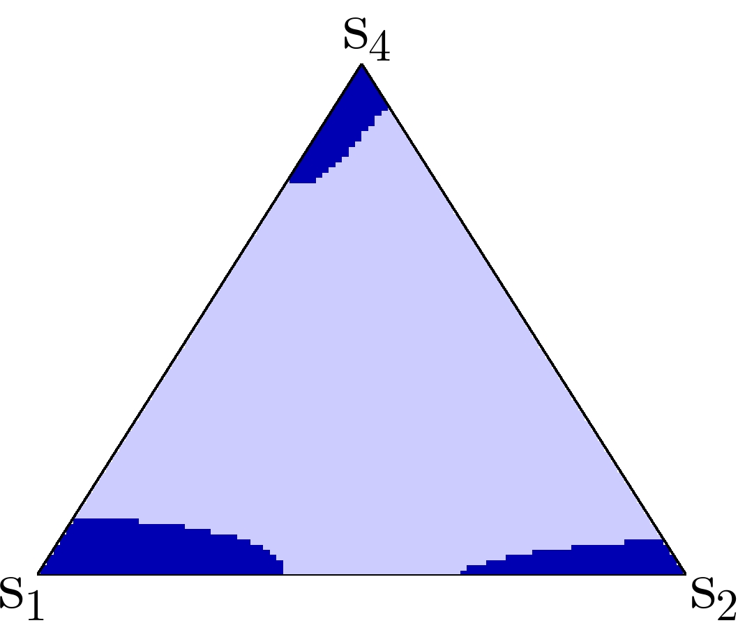
$|\mathcal{I}|=10$	$|\mathcal{I}|=10$	$|\mathcal{I}|=10$	$|\mathcal{I}|=10$

Figure 2: Generation of problems where $\ell_{1,2}$ succeeds, while $\ell_{1,1}$ fails. For a $20\times 60$ matrix $A$ and fixed support of size $|\mathcal{I}|=5,7,10$, we create vectors $f_{i}$ that cannot be recovered using $\ell_{1}$, and vectors $s_{i}$ than can be recovered. Each triangle represents an $X_{0}$ constructed from the vectors denoted in the corners. The location in the triangle determines the weight on each vector, ranging from zero to one, and summing up to one. The dark areas indicates the weights for which $\ell_{1,2}$ successfully recovered $X_{0}$.

4 Boosted $\ell_{1}$

As described in Section 3, recovery using $\ell_{1,1}$ is equivalent to individual $\ell_{1}$ recovery of each column $x_{k}:=X_{0}^{\scalebox{0.6}{$\downarrow$}{k}}$ based on $b_{k}\mathrel{\mathop{:}}=B^{\scalebox{0.6}{$\downarrow$}{k}}$, for $k=1,\ldots,r$:

$$\mathop{\hbox{minimize}}_{x}\quad\|x\|_{1}\quad\mathop{\hbox{subject to}}\quad Ax=b_{k}.$$ (4.1)

Assuming that the signs of nonzero entries in the support of each $x_{k}$ are drawn i.i.d. from $\{1,-1\}$, we can express the probability of recovering a matrix $X_{0}$ with row support $\mathcal{I}$ using $\ell_{1,1}$ in terms of the probability of recovering vectors on that support using $\ell_{1}$. To see how, note that $\ell_{1,1}$ recovers the original $X_{0}$ if and only if each individual problem in (4.1) successfully recovers each $x_{k}$. For the above class of matrices $X_{0}$ this therefore gives a recovery rate of

$$P_{\ell_{1,1}}(A,\mathcal{I},k)=\left[P_{\ell_{1}}(A,\mathcal{I})\right]^{r}.$$

Using $\ell_{1,1}$ to recover $X_{0}$ is clearly not a good idea. Note also that uniform recovery of $X_{0}$ on a support $\mathcal{I}$ remains unchanged, regardless of the number of observations, $r$, that are given. As a consequence of Theorem 3.2, this also means that the uniform-recovery properties for any sum-of-norms approach cannot increase with $r$. This clearly defeats the purpose of gathering multiple observations.

In many instances where $\ell_{1,1}$ fails, it may still recover a subset of columns $x_{k}$ from the corresponding observations $b_{k}$. It seems wasteful to discard this information because if we could recognize a single correctly recovered $x_{k}$, we would immediately know the row support $\mathcal{I}=\textrm{Supp}_{\mathrm{row}}(X_{0})=\textrm{Supp}(x_{k})$ of $X_{0}$. Given the correct support we can recover the nonzero part $\bar{X}$ of $X_{0}$ by solving

$$\mathop{\hbox{minimize}}_{\bar{X}}\quad\|A_{\mathcal{I}}\bar{X}-B\|_{F}.$$ (4.2)

In practice we obviously do not know the correct support, but when a given solution $x_{k}^{*}$ of (4.1) that is sufficiently sparse, we can try to solve (4.2) for that support and verify if the residual at the solution is zero. If so, we construct the final $X^{*}$ using the non-zero part and declare success. Otherwise we simply increment $k$ and repeat this process until there are no more observations and recovery was unsuccessful. We refer to this algorithm, which is reminiscent of the ReMBo approach [23], as boosted $\ell_{1}$; its sole aim is to provide a bridge to the analysis of ReMBo. The complete boosted $\ell_{1}$ algorithm is outlined in Figure 4.

The recovery properties of the boosted $\ell_{1}$ approach are opposite from those of $\ell_{1,1}$: it fails only if all individual columns fail to be recovered using $\ell_{1}$. Hence, given an unknown $n\times r$ matrix $X$ supported on $\mathcal{I}$ with its sign pattern uniformly random, the boosted $\ell_{1}$ algorithm gives an expected recovery rate of

$$P_{\ell_{1}^{B}}(A,\mathcal{I},r)=1-\left[1-P_{\ell_{1}}(A,\mathcal{I})\right]^{r}.$$ (4.3)

To experimentally verify this recovery rate, we generated a $20\times 80$ matrix $A$ with entries independently sampled from the normal distribution and fixed a randomly chosen support set $\mathcal{I}_{s}$ for three levels of sparsity, $s=8,9,10$. On each of these three supports we generated vectors with all possible sign patterns and solved (1.2) to see if they could be recovered or not (see Section 3.3). This gives exactly the face counts required to compute the $\ell_{1}$ recovery probability in (2.2), and the expected boosted $\ell_{1}$ recovery rate in (4.3)

For the empirical success rate we take the average over 1,000 trials with random coefficient matrices $X$ supported on $\mathcal{I}_{s}$, and its nonzero entries independently drawn from the normal distribution. To reduce the computational time we avoid solving $\ell_{1}$ and instead compare the sign pattern of the current solution $x_{k}$ against the information computed to determine the face counts (both $A$ and $\mathcal{I}_{s}$ remain fixed). The theoretical and empirical recovery rates using boosted $\ell_{1}$ are plotted in Figure 4.

given $A$, $B$ for $k=1,\ldots,r$ do solve (1.2) with $b_{k}=B^{\scalebox{0.6}{$\downarrow$}{k}}$ to get $x$ $\mathcal{I}\leftarrow\textrm{Supp}(x)$ if $|\mathcal{I}|<m/2$ then solve (4.2) to get $X$ if $A_{\mathcal{I}}X=B$ then $X^{*}=0$ $(X^{*})^{{j}{\scalebox{0.6}{$\rightarrow$}}}\leftarrow X^{{j}{\scalebox{0.6}{$\rightarrow$}}}$ for $j\in\mathcal{I}$ return solution $X^{*}$ return failure
Figure 3: The boosted $\ell_{1}$ algorithm	Figure 4: Theoretical (dashed) and experimental (solid) performance of boosted $\ell_{1}$ for three problem instances with different row support $s$.

5 Recovery using ReMBo

The boosted $\ell_{1}$ approach can be seen as a special case of the ReMBo [23] algorithm. ReMBo proceeds by taking a random vector $w\in\mathbb{R}^{r}$ and combining the individual observations in $B$ into a single weighted observation $b\mathrel{\mathop{:}}=Bw$. It then solves a single measurement vector problem $Ax=b$ for this $b$ (we shall use $\ell_{1}$ throughout) and checks if the computed solution $x^{*}$ is sufficiently sparse. If not, the above steps are repeated with a different weight vector $w$; the algorithm stops when a maximum number of trials is reached. If the support $\mathcal{I}$ of $x^{*}$ is small, we form $A_{\mathcal{I}}=[A^{\scalebox{0.6}{$\downarrow$}{j}}]_{j\in\mathcal{I}}$, and check if (4.2) has a solution $\bar{X}$ with zero residual. If this is the case we have the nonzero rows of the solution $X^{*}$ in $\bar{X}$ and are done. Otherwise, we simply proceed with the next $w$. The ReMBo algorithm reduces to boosted $\ell_{1}$ by limiting the number of iterations to $r$ and choosing $w=e_{i}$ in the $i$th iteration. We summarize the ReMBo-$\ell_{1}$ algorithm in Figure 6. The formulation given in [23] requires a user-defined threshold on the cardinality of the support $\mathcal{I}$ instead of the fixed threshold $m/2$. Ideally this threshold should be half of the spark [12] of A, where

$$\textrm{Spark}(A)\mathrel{\mathop{:}}=\min_{z\in\textrm{Ker}(A)\setminus\{0\}}\ \|z\|_{0}$$

which is the number of nonzeros of the sparsest vector in the kernel of $A$; any vector $x_{0}$ with fewer than $\textrm{Spark}(A)/2$ nonzeros is the unique sparsest solution of $Ax=Ax_{0}=b$ [12]. Unfortunately, the spark is prohibitively expensive to compute, but under the assumption that $A$ is in general position, $\textrm{Spark}(A)=m+1$. Note that choosing a higher value can help to recover signals with row sparsity exceeding $m/2$. However, in this case it can no longer be guaranteed to be the sparsest solution.

given $A$, $B$. Set $\mathrm{Iteration}\leftarrow 0$ while $\mathrm{Iteration}<\mathrm{MaxIteration}$ do $w\leftarrow\mathrm{Random}(n,1)$ solve (1.2) with $b=Bw$ to get $x$ $\mathcal{I}\leftarrow\textrm{Supp}(x)$ if $|\mathcal{I}|<m/2$ then solve (4.2) to get $X$ if $A_{\mathcal{I}}X=B$ then $X^{*}=0$ $(X^{*})^{{j}{\scalebox{0.6}{$\rightarrow$}}}\leftarrow X^{{j}{\scalebox{0.6}{$\rightarrow$}}}$ for $j\in\mathcal{I}$ return solution $X^{*}$ $\mathrm{Iteration}\leftarrow\mathrm{Iteration}+1$ return failure

Figure 5: The ReMBo-$\ell_{1}$ algorithm

Figure 6: Theoretical performance model for ReMBo on three problem instances with different sparsity levels $s$.

To derive the performance analysis of ReMBo, we fix a support $\mathcal{I}$ of cardinality $s$, and consider only signals with nonzero entries on this support. Each time we multiply $B$ by a weight vector $w$, we in fact create a new problem with an $s$-sparse solution $x_{0}=X_{0}w$ corresponding with a right-hand side $b=Bw=AX_{0}w=Ax_{0}$. As reflected in (2.2), recovery of $x_{0}$ using $\ell_{1}$ depends only on its support and sign pattern. Clearly, the more sign patterns in $x_{0}$ that we can generate, the higher the probability of recovery. Moreover, due to the elimination of previously tried sign patterns, the probability of recovery goes up with each new sign pattern (excluding negation of previous sign patterns). The maximum number of sign patterns we can check with boosted $\ell_{1}$ is the number of observations $r$. The question thus becomes, how many different sign patterns we can generate by taking linear combinations of the columns in $X_{0}$? (We disregard the situation where elimination occurs and $|\textrm{Supp}(X_{0}w)|<s$.) Equivalently, we can ask how many orthants in $\mathbb{R}^{s}$ (each one corresponding to a different sign pattern) can be properly intersected by the hyperplane given by the range of the $s\times r$ matrix $\bar{X}$ consisting of the nonzero rows of $X_{0}$ (with proper we mean intersection of the interior). In Section 5.1 we derive an exact expression for the maximum number of proper orthant intersections in $\mathbb{R}^{n}$ by a hyperplane generated by $d$ vectors, denoted by $C(n,d)$.

Based on the above reasoning, a good model for the recovery rate of $n\times r$ matrices $X_{0}$ with $\textrm{Supp}_{\mathrm{row}}(X_{0})=\mathcal{I}<m/2$ using ReMBo is given by

$$P_{\scriptscriptstyle R}(A,\mathcal{I},r)=1-\prod_{i=1}^{C(|\mathcal{I}|,r)/2}\left[1-\frac{\mathcal{F}_{\mathcal{I}}(A\mathcal{C})}{\mathcal{F}_{\mathcal{I}}(\mathcal{C})-2(i-1)}\right].$$ (5.1)

The term within brackets denotes the probability of failure and the fraction represents the success rate, which is given by the ratio of the number of faces $\mathcal{F}_{\mathcal{I}}(A\mathcal{C})$ that survived the mapping to the total number of faces to consider. The total number reduces by two at each trial because we can exclude the face $f$ we just tried, as well as $-f$. The factor of two in $C(|\mathcal{I}|,r)/2$ is also due to this symmetry.

This model would be a bound for the average performance of ReMBo if the sign patterns generated would be randomly sampled from the space of all sign patterns on the given support. However, because it is generated from the orthant intersections with a hyperplane, the actual pattern is highly structured. Indeed, it is possible to imagine a situation where the $(s-1)$-faces in $\mathcal{C}$ that perish in the mapping to $A\mathcal{C}$ have sign patterns that are all contained in the set generated by a single hyperplane. Any other set of sign patterns would then necessarily include some faces that survive the mapping and by trying all patterns in that set we would recover $X_{0}$. In this case, the average recovery over all $X_{0}$ on that support could be much higher than that given by (5.1). We do not yet fully understand how the surviving faces of $\mathcal{C}$ are distributed. Due to the simplicial structure of the facets of $\mathcal{C}$, we can expect the faces that perish to be partially clustered (if a $(d-2)$-face perishes, then so will the two $(d-1)$-faces whose intersection gives this face), and partially unclustered (the faces that perish while all their sub-faces survive). Note that, regardless of these patterns, recovery is guaranteed in the limit whenever the number of unique sign patterns tried exceeds half the number of faces lost, $(|\mathcal{F}_{\mathcal{I}}(\mathcal{C})|-|\mathcal{F}_{\mathcal{I}}(\mathcal{AC})|)/2$.

Figure 6 illustrates the theoretical performance model based on $C(n,d)$, for which we derive the exact expression in Section 5.1. In Section 5.2 we discuss practical limitations, and in Section 5.3 we empirically look at how the number of sign patterns generated grows with the number of normally distributed vectors $w$, and how this affects the recovery rates. To allow comparison between ReMBo and boosted $\ell_{1}$, we used the same matrix $A$ and support $\mathcal{I}_{s}$ used to generate Figure 4.

5.1 Maximum number of orthant intersections with subspace

Theorem 5.1.

Let $C(n,d)$ denote the maximum attainable number of orthant interiors intersected by a hyperplane in $\mathbb{R}^{n}$ generated by $d$ vectors. Then $C(n,1)=2$, $C(n,d)=2^{n}$ for $d\geq n$. In general, $C(n,d)$ is given by

$$C(n,d)=C(n-1,d-1)+C(n-1,d)=2\sum_{i=0}^{d-1}{n-1\choose i}.$$ (5.2)

Proof.

The number of intersected orthants is exactly equal to the number of proper sign patterns (excluding zero values) that can be generated by linear combinations of those $d$ vectors. When $d=1$, there can only be two such sign patterns corresponding to positive and negative multiples of that vector, thus giving $C(n,1)=2$. Whenever $d\geq n$, we can choose a basis for $\mathbb{R}^{n}$ and add additional vectors as needed, and we can reach all points, and therefore all $2^{n}=C(n,d)$ sign patterns.

For the general case (5.2), let $v_{1},\ldots,v_{d}$ be vectors in $\mathbb{R}^{n}$ such that the affine hull with the origin, $S=\mathrm{aff}\{0,v_{1},\ldots,v_{d}\}$, gives a hyperplane in $\mathbb{R}^{n}$ that properly intersects the maximum number of orthants, $C(n,d)$. Without loss of generality assume that vectors $v_{i}$, $i=1,\ldots,d-1$ all have their $n$th component equal to zero. Now, let $T=\mathrm{aff}\{0,v_{1},\ldots,v_{d-1}\}\subseteq\mathbb{R}^{n-1}$ be the intersection of $S$ with the $(n-1)$-dimensional subspace of all points $\mathcal{X}=\{x\in\mathbb{R}^{n}\mid x_{n}=0\}$, and let $C_{T}$ denote the number of $(n-1)$-orthants intersected by $T$. Note that $T$ itself, as embedded in $\mathbb{R}^{n}$, does not properly intersect any orthant. However, by adding or subtracting an arbitrarily small amount of $v_{d}$, we intersect $2C_{T}$ orthants; taking $v_{d}$ to be the $n$th column of the identity matrix would suffice for that matter. Any other orthants that are added have either $x_{n}>0$ or $x_{n}<0$, and their number does not depend on the magnitude of the $n$th entry of $v_{d}$, provided it remains nonzero. Because only the first $n-1$ entries of $v_{d}$ determine the maximum number of additional orthants, the problem reduces to $\mathbb{R}^{n-1}$. In fact, we ask how many new orthants can be added to $C_{T}$ taking the affine hull of $T$ with $v$, the orthogonal projection $v_{d}$ onto $\mathcal{X}$. Since the maximum orthants for this $d$-dimensional subspace in $\mathbb{R}^{n-1}$ is given by $C(n-1,d)$, this number is clearly bounded by $C(n-1,d)-C_{T}$. Adding this to $2C_{T}$, we have

$$C(n,d) \leq 2C_{T}+[C(n-1,d)-C_{T}]=C_{T}+C(n-1,d)$$ (5.3)

$$\leq C(n-1,d-1)+C(n-1,d)$$

$$\leq 2\sum_{i=0}^{d-1}{n-1\choose i}.$$

The final expression follows by expanding the recurrence relations, which generates (a part of) Pascal’s triangle, and combining this with $C(1,j)=2$ for $j\geq 1$. In the above, whenever there are free orthants in $\mathbb{R}^{n-1}$, that is, when $d<n$, we can always choose the corresponding part of $v_{d}$ in that orthant. As a consequence we have that no hyperplane supported by a set of vectors can intersect the maximum number of orthants when the range of those vectors includes some $e_{i}$.

We now show that this expression holds with equality. Let $U$ denote an $(n-d)$-hyperplane in $\mathbb{R}^{n}$ that intersects the maximum $C(n,n-d)$ orthants. We now claim that in the interior of each orthant not intersected by $U$ there exists a vector that is orthogonal to $U$. If this were not the case then $T$ must be aligned with some $e_{i}$ and can therefore not be optimal. The span of these orthogonal vectors generates a $d$-hyperplane $V$ that intersects $C_{V}=2^{n}-C(n,n-d)$ orthants, and it follows that

$$C(n,d) \geq C_{V}=2^{n}-C(n,n-d)$$

$$\geq 2^{n}-2\sum_{i=0}^{n-d-1}{n-1\choose i}=2\sum_{i=0}^{n-1}{n-1\choose i}-2\sum_{i=0}^{n-d-1}{n-1\choose i}$$

$$=2\sum_{n-d}^{n-1}{n-1\choose i}=2\sum_{i=0}^{d-1}{n-1\choose i}\geq C(n,d),$$

where the last inequality follows from (5.3). Consequently, all inequalities hold with equality. ∎

Corollary 5.2.

Given $d\leq n$, then $C(n,d)=2^{n}-C(n,n-d)$, and $C(2d,d)=2^{2d-1}$.

Corollary 5.3.

A hyperplane $\mathcal{H}$ in $\mathbb{R}^{n}$, defined as the range of $V=[v_{1},\ v_{2},\ldots,\ v_{d}]$, intersects the maximum number of orthants $C(n,d)$ whenever $\mathop{\hbox{\rm rank}}(V)=n$, or when $e_{i}\not\in\mathop{\hbox{\rm range}}(V)$ for $i=1,\ldots,n$.

5.2 Practical considerations

In practice it is generally not feasible to generate all of the $C(|\mathcal{I}|,r)/2$ unique sign patterns. This means that we would have to replace this term in (5.1) by the number of unique patterns actually tried. For a given $X_{0}$ the actual probability of recovery is determined by a number of factors. First of all, the linear combinations of the columns of the nonzero part of $\bar{X}$ prescribe a hyperplane and therefore a set of possible sign patterns. With each sign pattern is associated a face in $\mathcal{C}$ that may or may not map to a face in $A\mathcal{C}$. In addition, depending on the probability distribution from which the weight vectors $w$ are drawn, there is a certain probability for reaching each sign pattern. Summing the probability of reaching those patterns that can be recovered gives the probability $P(A,\mathcal{I},X_{0})$ of recovering with an individual random sample $w$. The probability of recovery after $t$ trials is then of the form

$$1-[1-P(A,\mathcal{I},X_{0})]^{t}.$$

To attain a certain sign pattern $\bar{e}$, we need to find an $r$-vector $w$ such that $\mathop{\hbox{\rm sign}}(\bar{X}w)=\bar{e}$. For a positive sign on the $j$th position of the support we can take any vector $w$ in the open halfspace $\{w\mid\bar{X}^{{j}{\scalebox{0.6}{$\rightarrow$}}}w>0\}$, and likewise for negative signs. The region of vectors $w$ in $\mathbb{R}^{r}$ that generates a desired sign pattern thus corresponds to the intersection of $|\mathcal{I}|$ open halfspaces. The measure of this intersection as a fraction of $\mathbb{R}^{r}$ determines the probability of sampling such a $w$. To formalize, define $\mathcal{K}$ as the cone generated by the rows of $-\mathop{\hbox{\rm diag}}(\bar{e})\bar{X}$, and the unit Euclidean $(k-1)$-sphere $\mathcal{S}^{k-1}=\{x\in\mathbb{R}^{r}\mid\|x\|_{2}=1\}$. The intersection of halfspaces then corresponds to the interior of the polar cone of $\mathcal{K}$: $\mathcal{K}^{\circ}=\{x\in\mathbb{R}^{r}\mid x^{T}\!y\leq 0,\ \forall y\in\mathcal{K}\}$. The fraction of $\mathbb{R}^{r}$ taken up by $\mathcal{K}^{\circ}$ is given by the $(k-1)$-content of $\mathcal{S}^{k-1}\cap\mathcal{K}^{\circ}$ to the $(k-1)$-content of $\mathcal{S}^{k-1}$ [21]. This quantity coincides precisely with the definition of the external angle of $\mathcal{K}$ at the origin.

5.3 Experiments

In this section we illustrate the theoretical results from Section 5 and examine some practical considerations that affect the performance of ReMBo. For all experiments that require the matrix $A$, we use the same $20\times 80$ matrix that was used in Section 4, and likewise for the supports $\mathcal{I}_{s}$. To solve (1.2), we again use CVX in conjunction with SDPT3. We consider $x_{0}$ to be recovered from $b=Ax_{0}=AX_{0}w$ if $\|x^{*}-x_{0}\|_{\infty}\leq 10^{-5}$, where $x^{*}$ is the computed solution.

The experiments that are concerned with the number of unique sign patterns generated depend only on the $s\times r$ matrix $\bar{X}$ representing the nonzero entries of $X_{0}$. Because an initial reordering of the rows does not affect the number of patterns, those experiments depend only on $\bar{X}$, $s=|\mathcal{I}|$, and the number of observations $r$; the exact indices in the support set $\mathcal{I}$ are irrelevant for those tests.

5.3.1 Generation of unique sign patterns

The practical performance of ReMBo depends on its ability to generate as many different sign patterns using the columns in $X_{0}$ as possible. A natural question to ask then is how the number of such patterns grows with the number of randomly drawn samples $w$. Although this ultimately depends on the distribution used for generating the entries in $w$, we shall, for sake of simplicity, consider only samples drawn from the normal distribution. As an experiment we take a $10\times 5$ matrix $\bar{X}$ with normally-distributed entries, and over $10^{8}$ trials record how often each sign-pattern (or negation) was reached, and in which trial they were first encountered. The results of this experiment are summarized in Figure 7. From the distribution in Figure 7(b) it is clear that the occurrence levels of different orthants exhibits a strong bias. The most frequently visited orthant pairs were reached up to $7.3\times 10^{6}$ times, while others, those hard to reach using weights from the normal distribution, were observed only four times over all trials. The efficiency of ReMBo depends on the rate of encountering new sign patterns. Figure 7(c) shows how the average rate changes over the number of trials. The curves in Figure 7(d) illustrate the theoretical probability of recovery in (5.1), with $C(n,d)/2$ replaced by the number of orthant pairs at a given iteration, and with face counts determined as in Section 4, for three instances with support cardinality $s=10$, and observations $r=5$.

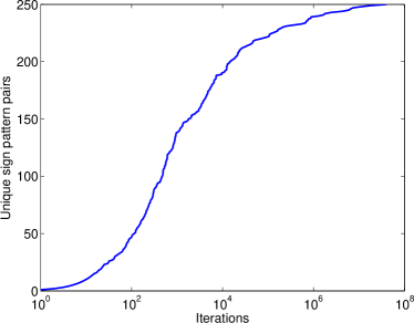
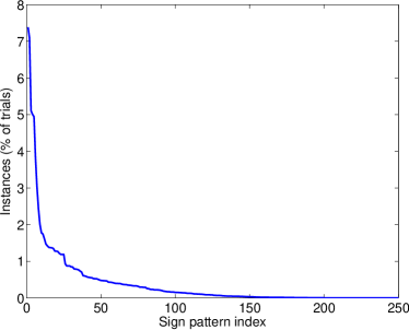
(a)	(b)
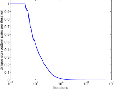
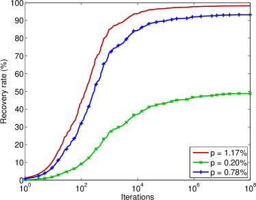
(c)	(d)

Figure 7: Sampling the sign patterns for a $10\times 5$ matrix $\bar{X}$, with (a) number of unique sign patterns versus number of trials, (b) relative frequency with which each orthant is sampled, (c) average number of new sign patterns per iteration as a function of iterations, and (d) theoretical probability of recovery using ReMBo for three instances of $X_{0}$ with row sparsity $s=10$, and $r=5$ observations.

5.3.2 Role of $\bar{X}$.

Although the number of orthants that a hyperplane can intersect does not depend on the basis with which it was generated, this choice does greatly influence the ability to sample those orthants. Figure 8 shows two ways in which this can happen. In part (a) we sampled the number of unique sign patterns for two different $9\times 5$ matrices $\bar{X}$, each with columns scaled to unit $\ell_{2}$-norm. The entries of the first matrix were independently drawn from the normal distribution, while those in the second were generated by repeating a single column drawn likewise and adding small random perturbations to each entry. This caused the average angle between any pair of columns to decrease from $65$ degrees in the random matrix to a mere $8$ in the perturbed matrix, and greatly reduces the probability of reaching certain orthants. The same idea applies to the case where $d\geq n$, as shown in part (b) of the same figure. Although choosing $d$ greater than $n$ does not increase the number of orthants that can be reached, it does make reaching them easier, thus allowing ReMBo to work more efficiently. Hence, we can expect ReMBo to have higher recovery on average when the number of columns in $X_{0}$ increases and when they have a lower mutual coherence $\mu(X)=\min_{i\neq j}|x_{i}^{T}x_{j}|/(\|x_{i}\|_{2}\cdot\|x_{j}\|_{2})$.

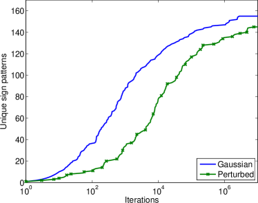
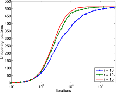
(a)	(b)

Figure 8: Number of unique sign patterns for (a) two $9\times 5$ matrices $\bar{X}$ with columns scaled to unit $\ell_{2}$-norm; one with entries drawn independently from the normal distribution, and one with a single random column repeated and random perturbations added, and (b) $10\times r$ matrices with $r=10,12,15$.

5.3.3 Limiting the number of iterations

The number of iterations used in the previous experiments greatly exceeds that what is practically feasible: we cannot afford to run ReMBo until all possible sign patterns have been tried, even if there was a way detect that the limit had been reached. Realistically, we should set the number of iterations to a fixed maximum that depends on the computational resources available, and the problem setting.

In Figure 7 we show the unique orthant count as a function of iterations and the predicted recovery rate. When using only a limited number of iterations it is interesting to know what the distribution of unique orthant counts looks like. To find out, we drew 1,000 random $\bar{X}$ matrices for each size $s\times r$, with $s=10$ nonzero rows fixed, and the number of columns ranging from $r=1,\ldots,20$. For each $\bar{X}$ we counted the number of unique sign patterns attained after respectively 1,000 and 10,000 iterations. The resulting minimum, maximum, and median values are plotted in Figure 9(a) along with the theoretical maximum. More interestingly of course is the average recovery rate of ReMBo with those number of iterations. For this test we again used the $20\times 80$ matrix $A$ with predetermined support $\mathcal{I}$, and with success or failure of each sign pattern on that support precomputed. For each value of $r=1,\ldots,20$ we generated random matrices $X$ on $\mathcal{I}$ and ran ReMBo with the maximum number of iterations set to 1,000 and 10,000. To save on computing time, we compared the on-support sign pattern of each combined coefficient vector $Xw$ to the known results instead of solving $\ell_{1}$. The average recovery rate thus obtained is plotted in Figures 9(b)–(c), along with the average of the predicted performance using (5.1) with $C(n,d)/2$ replaced by orthant counts found in the previous experiment.

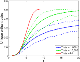
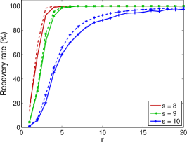
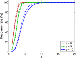
(a)	(b)	(c)

Figure 9: Effect of limiting the number of weight vectors $w$ on (a) the distribution of unique orthant counts for $10\times k$ random matrices $\bar{X}$, solid lines give the median number and the dashed lines indicate the minimum and maximum values, the top solid line is the theoretical maximum; (b–c) the average performance of the ReMBo-$\ell_{1}$ algorithm (solid) for fixed $20\times 80$ matrix $A$ and three different support sizes $r=8,9,10$, along with the average predicted performance (dashed). The support patterns used are the same as those used for Figure 4.

6 Conclusions

The MMV problem is often solved by minimizing the sum-of-row norms of the unknown coefficients $X$. We show that the (local) uniform recovery properties, i.e., recovery of all $X_{0}$ with a fixed row support $\mathcal{I}=\textrm{Supp}_{\mathrm{row}}(X_{0})$, cannot exceed that of $\ell_{1,1}$, the sum of $\ell_{1}$ norms. This is despite the fact that $\ell_{1,1}$ reduces to solving the basis pursuit problem (1.2) for each column separately, which does not take advantage of the fact that all vectors in $X_{0}$ are assumed to have the same support. A consequence of this observation is that the use of restricted isometry techniques to analyze (local) uniform recovery using sum-of-norm minimization can at best give improved bounds on $\ell_{1}$ recovery.

Empirically, minimization with $\ell_{1,2}$, the sum of $\ell_{2}$ norms, clearly outperforms $\ell_{1,1}$ on individual problem instances: for supports where uniform recovery fails, $\ell_{1,2}$ recovers more cases than $\ell_{1,1}$. We construct cases where $\ell_{1,2}$ succeeds while $\ell_{1,1}$ fails, and vice versa. From the construction where only $\ell_{1,2}$ succeeds it also follows that the relative magnitudes of the coefficients in $X_{0}$ matter for recovery. This is unlike $\ell_{1,1}$ recovery, where only the support and the sign patterns matter. This implies that the notion of faces, so useful in the analysis of $\ell_{1}$, disappears.

We show that the performance of $\ell_{1,1}$ outside the uniform-recovery regime degrades rapidly as the number of observations increases. We can turn this situation around, and increase the performance with the number of observations by using a boosted-$\ell_{1}$ approach. This technique aims to uncover the correct support based on basis pursuit solutions for individual observations. Boosted-$\ell_{1}$ is a special case of the ReMBo algorithm which repeatedly takes random combinations of the observations, allowing it to sample many more sign patterns in the coefficient space. As a result, the potential recovery rates of ReMBo (at least in combination with an $\ell_{1}$ solver) are a much higher than boosted-$\ell_{1}$. ReMBo can be used in combination with any solver for the single measurement problem $Ax=b$, including greedy approaches and reweighted $\ell_{1}$ [4]. The recovery rate of greedy approaches may be lower than $\ell_{1}$ but the algorithms are generally much faster, thus giving ReMBo the chance to sample more random combinations. Another advantage of ReMBo, even more so than boosted-$\ell_{1}$, is that it can be easily parallelized.

Based on the geometrical interpretation of ReMBo-$\ell_{1}$ (cf. Figure 6), we conclude that, theoretically, its performance does not increase with the number of observations after this number reaches the number of nonzero rows. In addition we develop a simplified model for the performance of ReMBo-$\ell_{1}$. To improve the model we would need to know the distribution of faces in the cross-polytope $\mathcal{C}$ that map to faces on $A\mathcal{C}$, and the distribution of external angles for the cones generated by the signed rows of the nonzero part of $X_{0}$.

It would be very interesting to compare the recovery performance between $\ell_{1,2}$ and ReMBo-$\ell_{1}$. However, we consider this beyond the scope of this paper.

All of the numerical experiments in this paper are reproducible. The scripts used to run the experiments and generate the figures can be downloaded from

http://www.cs.ubc.ca/~mpf/jointsparse.

References

- [1] E. J. Candès. Compressive sampling. In Proceedings of the International Congress of Mathematicians, Madrid, Spain, 2006.
- [2] E. J. Candès, J. Romberg, and T. Tao. Robust uncertainty principles: Exact signal reconstruction from highly incomplete frequency information. IEEE Transactions on Information Theory, 52(2):489–509, February 2006.
- [3] E. J. Candès and T. Tao. Decoding by linear programming. IEEE Transactions on Information Theory, 51(2):4203–4215, December 2005.
- [4] E. J. Candès, M. B. Wakin, and S. P. Boyd. Enhancing sparsity by reweighted minimization. Journal of Fourier Analysis and Applications, 14(5–6):877–905, December 2008.
- [5] J. Chen and X. Huo. Theoretical results on sparse represenations of multiple-measurement vectors. IEEE Transactions on Signal Processing, 54:4634–4643, December 2006.
- [6] S. S. Chen, D. L. Donoho, and M. A. Saunders. Atomic decomposition by basis pursuit. SIAM Journal on Scientific Computing, 20(1):33–61, 1998.
- [7] S. F. Cotter and B. D. Rao. Sparse channel estimation via matching pursuit with application to equalization. IEEE Transactions on Communications, 50(3), March 2002.
- [8] S. F. Cotter, B. D. Rao, K. Engang, and K. Kreutz-Delgado. Sparse solutions to linear inverse problems with multiple measurement vectors. IEEE Transactions on Signal Processing, 53:2477–2488, July 2005.
- [9] D. L. Donoho. Neighborly polytopes and sparse solution of underdetermined linear equations. Technical Report 2005-4, Department of Statistics, Stanford University, Stanford, CA, 2005.
- [10] D. L. Donoho. Compressed sensing. IEEE Transactions on Information Theory, 52(4):1289–1306, April 2006.
- [11] D. L. Donoho. High-dimensional centrosymmetric polytopes with neighborliness proportional to dimension. Discrete and Computational Geometry, 35(4):617–652, May 2006.
- [12] D. L. Donoho and M. Elad. Optimally sparse representation in general (nonorthogonal) dictionaries via minimization. PNAS, 100(5):2197–2202, March 2003.
- [13] D. L. Donoho and X. Huo. Uncertainty principles and ideal atomic decomposition. IEEE Transactions on Information Theory, 47(7):2845–2862, November 2001.
- [14] Y. C. Eldar and M. Mishali. Robust recovery of signals from a union of subspaces. arXiv 0807.4581, July 2008.
- [15] I. J. Fevrier, S. B. Gelfand, and M. P. Fitz. Reduced complexity decision feedback equalization for multipath channels with large delay spreads. IEEE Transactions on Communications, 47(6):927–937, June 1999.
- [16] J.-J. Fuchs. On sparse representations in arbitrary redundant bases. IEEE Transactions on Information Theory, 50(6):1341–1344, June 2004.
- [17] M. Grant and S. Boyd. Graph implementations for nonsmooth convex programs. In V. Blondel, S. Boyd, and H. Kimura, editors, Lecture Notes in Control and Information Sciences, pages 95–110. Springer, 2008.
- [18] M. Grant and S. Boyd. CVX: Matlab software for disciplined convex programming (web page and software). http://stanford.edu/~boyd/cvx, February 2009.
- [19] R. Gribonval and M. Nielsen. Sparse representations in unions of bases. IEEE Transactions on Information Theory, 49(12):3320–3325, December 2003.
- [20] R. Gribonval and M. Nielsen. Highly sparse representations from dictionaries are unique and independents of the sparseness measure. Applied and Computational Harmonic Analysis, 22(3):335–355, May 2007.
- [21] B. Grünbaum. Convex Polytopes, volume 221 of Graduate Texts in Mathematics. Springer-Verlag, second edition, 2003.
- [22] D. Malioutov, M. Çetin, and A. S. Willsky. A sparse signal reconstruction perspective for source localization with sensor arrays. IEEE Transactions on Signal Processing, 53(8):3010–3022, August 2005.
- [23] M. Mishali and Y. C. Eldar. Reduce and boost: Recovering arbitrary sets of jointly sparse vectors. IEEE Transactions on Signal Processing, 56(10):4692–4702, October 2008.
- [24] B. K. Natarajan. Sparse approximate solutions to linear systems. SIAM Journal on Computing, 24(2):227–234, April 1995.
- [25] R. T. Rockafellar. Convex Analysis. Princeton University Press, Princeton, 1970.
- [26] M. Stojnic, F. Parvaresh, and B. Hassibi. On the reconstruction of block-sparse signals with an optimal number of measurements. arXiv 0804.0041, March 2008.
- [27] J. A. Tropp. Recovery of short, complex linear combinations via minimization. IEEE Transactions on Information Theory, 51(4):1568–1570, April 2005.
- [28] J. A. Tropp. Algorithms for simultaneous sparse approximation: Part II: Convex relaxation. Signal Processing, 86:589–602, 2006.
- [29] J. A. Tropp, A. C. Gilbert, and M. J. Strauss. Algorithms for simultaneous sparse approximation: Part I: Greedy pursuit. Signal Processing, 86:572–588, 2006.
- [30] R. H. Tütüncü, K. C. Toh, and M. J. Todd. Solving semidefinite-quadratic-linear programs using SDPT3. Mathematical Programming Ser. B, 95:189–217, 2003.