Equilibrium Configurations of Relativistic stars with purely toroidal magnetic fields : effects of realistic equations of state

Abstract

We investigate equilibrium sequences of relativistic stars containing purely toroidal magnetic fields with four kinds of realistic equations of state (EOSs) of SLy (Douchin et al.), FPS (Pandharipande et al.), Shen (Shen et al.), and LS (Lattimer & Swesty). We numerically construct thousands of equilibrium configurations in order to study the effects of the realistic EOSs. Particularly we pay attention to the equilibrium sequences of constant baryon mass and/or constant magnetic flux, which model evolutions of an isolated neutron star, losing angular momentum via gravitational waves. Important properties obtained in this study are summarized as follows ; (1) Unlike the polytropic EOS, it is found for the realistic EOSs that the maximum masses do not monotonically increase with the field strength along the constant magnetic flux sequences. (2) The dependence of the mass-shedding angular velocity on the EOSs is determined from that of the non-magnetized case. The stars with Shen(FPS) EOS reach the mass-shedding limit at the smallest(largest) angular velocity, while the stars with SLy or Lattimer-Swesty EOSs take the moderate values. (3) For the supramassive sequences, the equilibrium configurations are found to be generally oblate for the realistic EOSs in sharp contrast to the polytropic stars. For FPS(LS) EOS, the parameter region which permits the prolately deformed stars is widest(narrowest). For SLy and Shen EOS, it is in medium. Furthermore, the angular velocities $\Omega_{\rm up}$, above which the stars start to spin up as they lose angular momentum, are found to depend sharply on the realistic EOSs. Our analysis indicates that the hierarchy of this spin up angular velocity is $\Omega_{\rm up,SLy}>\Omega_{\rm up,FPS}>\Omega_{\rm up,LS}>\Omega_{\rm up,Shen}$ and this relation holds even if the sequences have strong magnetic fields. Our results suggest the relativistic stars containing purely toroidal magnetic fields will be a potential source of gravitational waves and the EOSs within such stars can be constrained by observing the angular velocity, the gravitational wave, and the signature of the spin up.

1. Introduction

Neutron stars observed in nature are magnetized with the typical magnetic field strength $\sim 10^{11}$–$10^{13}$ G (Lyne & Graham-Smith, 2005). For a special class of the neutron stars such as soft gamma-ray repeaters (SGRs) and anomalous X-ray pulsars (AXPs), the field strength is often much larger than the canonical value as $\sim 10^{15}$ G, and these objects are collectively referred as magnetars (Lattimer & Prakash, 2007; Woods & Thompson, 2004). Although such stars are estimated to be only a subclass ($\sim 10\%$) of the canonical neutron stars (Kouveliotou, 1998), much attention has been drawn because they pose many astrophysically exciting but unresolved problems.

Giant flaring activities observed in the SGRs have given us good opportunities to study the coupling of the interior to the magnetospheric structures (Thompson & Duncan, 1995, 1996), but we still know little of the relationship between the crustal fraction and the subsequent starquakes (see references in Watts (2006); Geppert & Rheinhardt (2006)). The origin of the large magnetic field is also a big problem, whether descended from the main sequence stars (Ferrario & Wickramasinghe, 2006) or generated at post-collapse in the rapidly rotating neutron star (Thompson & Duncan, 1993). Assuming large magnetic fields before core-collapse, extensive magnetohydrodynamic (MHD) stellar collapse simulations have been carried out recently (Kotake et al., 2004; Obergaulinger et al., 2006; Shibata et al., 2006; Livne et al., 2007; Dessart et al., 2007; Takiwaki et al., 2004; Sawai et al., 2008; Kiuchi et al., 2008; Takiwaki et al., 2009) towards the understanding of the formation mechanism of magnetars. Here it is worth mentioning that the gravitational waves could be a useful tool to supply us with the information about magnetar interiors (Bonazzola & Gourgoulhon, 1996; Cutler, 2002). While in a microscopic point of view, effects of magnetic fields larger than the so-called QED limit of $B_{\rm QED}=4.4\times 10^{13}~{}\rm{G}$, on the EOSs (e.g., Lattimer & Prakash (2007)) and the radiation processes have been also elaborately investigated (see Harding & Lai (2006) for a review). For the understanding of the formation and evolution of the magnetars, the unification of these macroscopic and microscopic studies is necessary, albeit not an easy task.

In order to investigate those fascinating issues, the construction of the equilibrium configuration of magnetars may be one of the most fundamental problems. Starting from the pioneering study by Chandrasekhar & Fermi (1953), extensive studies have been done and this research field is now experiencing ”renaissance” (Boucquet et al., 1995; Ioka & Sasaki, 2003, 2004; Kiuchi & Kotake, 2008; Konno et al., 1999; Tomimura & Eriguchi, 2005; Yoshida & Eriguchi, 2006; Yoshida et al., 2006), in which different levels of sophistication in the treatment of the magnetic field structure, equations of state (EOSs), and the general relativity, have been undertaken. Among them, a more sophistication is required for the studies employing the Newtonian gravity, because the general relativity(GR) should play an important role for the equilibrium configurations of compact objects like neutron stars. As mentioned below, typical densities for neutron stars interior exceed the nuclear density $\sim 10^{14}{\rm g/cm^{3}}$. In such a high density region, the pressure $P$ and rest mass density $\rho_{0}$ becomes comparable, namely $P\sim\rho_{0}c^{2}$ with $c$ being the speed of light. In such a regime, the Newtonian gravity is too weak to gravitationally bind the neutron stars without the general relativity, that is $GM/c^{2}R$ becomes the orders of magnitude $10^{-1}$ with $G$, $M$ and $R$ being gravitational constant, mass and radius of star.

It is noted here that the equilibrium configurations of relativistic stars without magnetic fields have been elaborately studied using the LORENE code (Bonazzola et al., 1998). Unfortunately, however, the method of constructing a fully general relativistic star with arbitrarily magnetic structures is still not available. In most previous studies, the weak magnetic fields and/or purely poloidal magnetic fields have been assumed. Boucquet et al. (1995) and Cardall et al. (2001) have treated relativistic stellar models containing purely poloidal magnetic fields. Konno et al. (1999) have analyzed similar models using a perturbative approach. Ioka & Sasaki (2004) have investigated structures of mixed poloidal-toroidal magnetic fields around a spherical star by using a perturbative technique.

As shown in the MHD simulations of core-collapse supernovae (see Kotake et al. (2006) for a review), the toroidal magnetic fields can be efficiently amplified due to the winding of the initial seed poloidal fields as long as the core rotates differentially. After core bounce, as a result, the toroidal fields generically dominate over the poloidal ones even if there is no toroidal field initially. Even for the weakly magnetized star prior to core-collapse, it should be mentioned that the magnetorotational instability (Balbus & Hawley, 1991) could be another effective mechanism for generating large toroidal magnetic fields (Akiyama et al., 2003). As pointed by Spruit (2007), such large magnetic fields generated by those processes may be confined inside the neutron star for thousands of years. Moreover, recent calculations of stellar evolution suggest that toroidal component of magnetic field dominates over poloidal one with the orders of magnitude $10^{-4}$ in the newly born neutron star after supernova explosion (Heger et al., 2005). These outcomes seem to indicate that some neutron stars could have toroidal fields much higher than the poloidal ones, which motivated Kiuchi & Yoshida (2008) to study the equilibrium configurations with purely toroidal fields. In the study, the master equations were derived for the first time for obtaining the relativistic rotating stars with the toroidal fields. On the other hand, it is well known that pure toroidal magnetic field in star is unstable (Tayler, 1973). Braithwaite & Spruit (2004) have investigated the evolution of magnetic field in stellar interior and found “twisted torus” field configuration is stable, in which the poloidal and toroidal magnetic field have comparable field strength. Recently, Kiuchi et al. (2008) have confirmed the Tayler instability in the neutron stars with the general relativistic magnetohydrodynamics simulation (GRMHD) under axisymmetric condition. Important finding of this study is the toroidal magnetic fields settle down to the new equilibrium states with the circular motion in meridian plane. This suggests that the toroidal magnetic field may remain in neutron stars even if the poloidal magnetic field is much weaker than the toroidal one.

However there may remain a room yet to be sophisticated in Kiuchi & Yoshida (2008) that the polytropic EOSs have been used for simplicity. In general, the central density of neutron stars is considered to be higher than the nuclear saturation density (Baym & Pethick, 1979). Since we still do not have an definite answer about the EOS in such a higher regime, many kinds of the nuclear EOSs have been proposed (e.g., Lattimer & Prakash (2007)) depending on the descriptions of the nuclear forces and the possible appearance of the exotic physics (e.g., Glendenning (2001)). While the stiffness of the polytropic EOS is kept constant globally inside the star, it should depend on the density in the realistic EOSs. Since the equilibrium configurations are achieved by the subtle and local balance of the gravitational force, centrifugal force, the Lorentz force, and the pressure gradient, it is a nontrivial problem how the equilibrium configurations change for the realistic EOSs.

These situations motivate us to study the effects of the realistic EOSs on the general relativistic stellar equilibrium configurations with purely toroidal magnetic fields. For the purpose, we incorporate the realistic EOSs to the numerical scheme by Kiuchi & Yoshida (2008). Four kinds of EOSs, of SLy (Douchin & Haensel, 2001), FPS (Pandharipande & Ravenhall, 1989), Shen (Shen et al., 1998a), and Lattimer-Swesty(LS) (Lattimer & Swesty, 1991) are adopted, which are often employed in the recent MHD studies relevant for magnetars. By so doing, we construct thousands of equilibrium stars for a wide range of parameters with different kinds of EOSs. As shown by Trehan & Uberoi (1972), the toroidal field tends to distort a stellar shape prolately because the toroidal field lines behave like a rubber belt, pulling in the matter around the magnetic axis. Such a prolate-shaped neutron star is pointed out to be optimal gravitational-waves emitters, depending on the degree of the prolateness (Cutler, 2002). Thus, we pay attention to how the prolateness is affected by the realistic EOSs. For making such configurations, maximum magnetic field strength deep inside the magnetars can become as high as $10^{18}$ G, which could be generated due to $\alpha-\Omega$ dynamos in the rapidly rotating neutron stars (Thompson & Duncan, 1993, 1996). It should be noted that the possibility of such ultra-magnetic fields has not been rejected so far, because what we can learn from the magnetar’s observations by their periods and spin-down rates is only their surface fields ($\sim 10^{15}$ G) . We construct equilibrium sequences, along which the total baryon rest mass and/or the magnetic flux with respect to the meridional cross-section keep constant. It has been suggested that the magnetic field will decay by the process of the Ohmic decay, ambipolar diffusion, and Hall drift (e.g., Goldreich & Reisenegger (1992)). This implies the magnetic flux might not be well conserved during quasi-steady evolution of isolated neutron stars. However, taking account into these effect to the neutron star’s evolution requires extensive efforts. Hence, as a first approximation, we explore the evolutionary sequences by use of the equilibrium sequences of constant rest mass and magnetic flux.

This paper is organized as follows. The master equations for obtaining equilibrium configurations of rotating stars with purely toroidal magnetic fields are briefly reviewed in Sec. 2. The numerical scheme for computing the stellar models and EOSs we employ in this study are briefly described in Sec. 3. Sec. 4 is devoted to showing numerical results. Summary and discussion follow in Sec. 5. In this paper, we use geometrical units with $G=c=1$.

2. Summary of basic equations

Master equations for the rotating relativistic stars containing purely toroidal magnetic fields have been derived in Kiuchi & Yoshida (2008). Hence, we only give a brief summary for later convenience.

Assumptions to obtain the equilibrium models are summarized as follows ; (1) Equilibrium models are stationary and axisymmetric. (2) The matter source is approximated by a perfect fluid with infinite conductivity. (3) There is no meridional flow of the matter. (4) The equation of state for the matter is barotropic. Although we employ realistic EOSs in this paper, this barotropic condition can be maintained as explained in subsection 3.2. (5) The magnetic axis and rotation axis are aligned.

Because the circularity condition (see, e.g. Wald (1984)) holds under these assumptions, the metric can be written, following Komatsu et al. (1989) and Cook et al. (1992), in the form,

$$ds^{2}=-{\rm e}^{\gamma+\rho}dt^{2}+{\rm e}^{2\alpha}(dr^{2}+r^{2}d\theta^{2})+{\rm e}^{\gamma-\rho}r^{2}\sin^{2}\theta(d\varphi-\omega dt)^{2},$$ (1)

where the metric potentials, $\gamma$, $\rho$, $\alpha$, and $\omega$, are functions of $r$ and $\theta$ only. We see that the non-zero component of Faraday tensor $F_{\mu\nu}$ in this coordinate is $F_{12}$. In case of purely toroidal magnetic field, the Grad-Shafranov equation is known to be trivial because it is given only in terms of the $\varphi$ component of the vector potential (see Kiuchi & Yoshida (2008) for details). Then the toroidal magnetic field can be determined by the integrability condition of the equation of motion (see Eq.(3)). Integrability of the equation of motion of the matter requires,

$$e^{\gamma-2\alpha}\sin\theta F_{12}=K(u);~{}~{}~{}u\equiv\rho_{0}he^{2\gamma}r^{2}\sin^{2}\theta,$$ (2)

where $K$ is an arbitrary function of $\rho_{0}he^{2\gamma}r^{2}\sin^{2}\theta$. The variables $\rho_{0}$ and $h$ represent the rest mass density and relativistic specific enthalpy, respectively. Integrating the equation of motion of the matter, we arrive at the equation of hydrostatic equilibrium,

$$\ln h+\frac{\rho+\gamma}{2}+\frac{1}{2}\ln(1-v^{2})+\frac{1}{4\pi}\int\frac{K(u)}{u}\frac{dK}{du}du=C,$$ (3)

where $v=(\Omega-\omega)r\sin\theta{\rm e}^{-\rho}$ with $\Omega$ being the angular velocity of the matter and $C$ is an integration constant.

Here, we have further assumed the rigid rotation. To compute specific models of the magnetized stars, we need specify the function forms of $K$, which determines the distribution of the magnetic fields. According to Kiuchi & Yoshida (2008), we take the following simple form,

$$K(u)=bu^{k},$$ (4)

where $b$ and $k$ are constants. Regularity of toroidal magnetic fields on the magnetic axis requires that $k\geq 1$. If $k\geq 1$, the magnetic fields automatically vanish at the surface of the star. Kiuchi & Yoshida (2008) have investigated how the choice of $k$ affects the magnetic field distribution. In this study, we consider the $k=1$ case because in the general relativistic MHD simulation, Kiuchi et al. (2008) have found that magnetic distribution with $k\neq 1$ is unstable against axisymmetric perturbations. Note that Tayler (1973) has suggested that the magnetic field configuration of $k=1$ is unstable against non-axisymmetric perturbations.

3. Numerical Method and Equation of State

3.1. Numerical method

To solve the master equations numerically, we employ the Kiuchi-Yoshida scheme (Kiuchi & Yoshida, 2008), which does not care about the function form of EOS. Hence, it is straight forward to update our numerical code for incorporating the realistic EOSs discussed below.

After obtaining solutions, it is useful to compute global physical quantities characterizing the equilibrium configurations to clearly understand the properties of the sequences of the equilibrium models. In this paper, we compute the following quantities: the gravitational mass $M$, the baryon rest mass $M_{0}$, the total angular momentum $J$, the total rotational energy $T$, the total magnetic energy $H$, the magnetic flux $\Phi$, the gravitational energy $W$ and the mean deformation rate $\bar{e}$, whose definitions are explicitly given in Kiuchi & Yoshida (2008). More explicitly, the mean deformation rate $\bar{e}$ is defined as

$$\bar{e}\equiv\frac{I_{zz}-I_{xx}}{I_{zz}},$$ (5)

where $I_{xx}=\pi\int\epsilon r^{4}\sin\theta(1+\cos^{2}\theta)drd\theta$ and $I_{zz}=2\pi\int\epsilon r^{4}\sin^{3}\theta drd\theta$ with $\epsilon$ being the energy density of the matter. (g) Circumferential radius $R_{\rm cir}$ is defined as $R_{\rm cir}\equiv{\rm e}^{(\gamma-\rho)/2}r_{e}$ with $r_{e}$ being the coordinate radius at the stellar equatorial surface. For all the models, checking the relativistic virial identities  (Bonazzola & Gourgoulhon, 1994; Gourgoulhon & Bonazzola, 1994), we confirm the typical values are orders of magnitude $10^{-4}-10^{-3}$, which are acceptable values for present numerical scheme.

3.2. Equations of State

As mentioned in Sec. 1, equation of state (EOS) is an important ingredient for determining the equilibrium configurations. Instead of conducting an extensive study as done before for the studies of rotating equilibrium configurations in which a greater variety of EOSs were employed, (e.g., Nozawa et al. (1998); Morrison et al. (2004) and references therein), we adopt here four kinds of EOSs, of SLy (Douchin & Haensel, 2001), FPS (Pandharipande & Ravenhall, 1989), Shen (Shen et al., 1998a), and Lattimer-Swesty(LS) (Lattimer & Swesty, 1991), which are often employed in the recent MHD studies relevant for magnetars.

In the study of cold neutron stars, the $\beta$-equilibrium condition with respect to beta decays of the form $e^{-}+p\longleftrightarrow n+\nu_{e}$ and $n\longleftrightarrow p+e^{-}+\bar{\nu}_{e}$, can be well validated as for the static properties. Since neutrinos and antineutrinos escape from the star, their chemical potentials vanish at zero-temperature $T=0$ with $T$ being the temperature. Thus the $\beta$-equilibrium condition can be expressed as $\mu_{\rm n}=\mu_{\rm e}+\mu_{\rm p}$, with $\mu_{\rm n}$, $\mu_{\rm e}$, and $\mu_{\rm p}$ being the chemical potentials of neutron, electron, and proton, respectively. With the charge neutrality condition, we can determine the three independent thermodynamic variables, (for example the pressure as $P(\rho,Y_{e},T)$, with $Y_{e}$ being the electron fraction), can only be determined by a single variable, which we take to be the density, namely $P(\rho,Y_{e}(\rho))$ (Shapiro & Teukolsky, 1983), noting here that $T=0$ is assumed for the case of the cold neutron stars. Thanks to this, we can use the formalism mentioned in Sec. 2 without violating the barotropic condition of the EOSs. It should be noted that Reisenegger (2008) has recently argued the breaking of the barotropic condition leads to the stabilization of the magnetic equilibria. This tells us the importance to model the neutron stars by multicomponent fluid, such as neutrons, electrons, and protons (Reisenegger, 2001). However, taking into account this effect to equilibrium configuration is beyond scope of this article. Furthermore, the barotropic condition plays a crucial role to obtain the Bernoulli equation Eq. (3). Hence, in this article, we only consider the barotropic case for simplicity.

At the maximum densities higher than $\sim 2\rho_{\rm nuc}$, muons can appear, and higher than $\sim 3\rho_{\rm nuc}$ (Wiringa et al., 1988; Akmal & Pahdharipahde, 1998), one may take into the possible appearance of hyperons (Glendenning, 2001). However, since the muon contribution to pressure at the higher density has been pointed to be very small (Douchin & Haensel, 2001), and we still do not have detailed knowledge of the hyperon interactions, we prefer to employ the above neutron star matter, namely $e^{-},n,p$, model to higher densities. In the following, we shortly summarize features of the EOSs employed here.

The Lattimer-Swesty EOS (Lattimer & Swesty, 1991) has been used for many years as a standard in the research field of core-collapse supernova explosions and the subsequent neutron star formations (see references in Sumiyoshi et al. (2005); Kotake et al. (2006)); it is based on the compressible drop model for nuclei together with dripped nucleons. The values of nuclear parameters are chosen according to nuclear mass formulae and other theoretical studies with the Skyrme interaction. The Shen EOS (Shen et al., 1998a) is a rather modern one and currently often used in the research field. The Shen EOS is based on the relativistic mean field theory with a local density approximations, which has been constructed to reproduce the experimental data of masses and radii of stable and unstable nuclei (see references in Shen et al. (1998a)). FPS are modern version of an earlier microscopic EOS calculations by Friedman & Pandharipande (1981), which employs both two body (U14) and three-body interactions (TNI). In the SLy EOS (Douchin & Haensel, 2001), neutron-excess dependence is added to the FPS EOS, which is more suitable for the neutron star interiors. As for the FPS and SLy EOSs, we use the fitting formulae presented in Shibata et al. (2005).

4. Numerical Results

In constructing one equilibrium sequence, we have three parameters to choose, namely the central density $\rho_{c}$, the strength of the magnetic field parameter $b$, and the axis ratio $r_{p}/r_{e}$. Changing these parameters, we have to seek solutions in as wide parameter range as possible to study the properties of the equilibrium sequences in detail. For clarity, we categorize the computed models into two, namely, non-rotating or rotating and discuss them separately, as done in Kiuchi & Yoshida (2008).

To calculate the non-rotating models, $\rho_{c}$ and $b$ (see Eq. (4)) have to be given with $\Omega=0$, where $\Omega$ is the angular velocity. For the rotating models, one need specify the axis ratio $r_{p}/r_{e}$ in addition to $\rho_{c}$ and $b$, where $r_{p}$ and $r_{e}$ are the polar and the equatorial radii, respectively. To explore properties of the relativistic magnetized star models with the realistic EOSs, we construct thousands of the equilibrium models for each EOS, namely for the non-rotating cases, $28\times 40$ models in the parameter space of $(\rho_{c},\ b)$, and for the rotating cases, $28\times 40\times 10$ models in the parameter space of $(\rho_{c},\ b,\ r_{p}/r_{e})$. Throughout this section, we mainly pay attention to the magnetic field dominant models, i.e., the models with $H>T$, since we are concerned with the structure of the magnetar. For some magnetars, the condition of $H>T$ could be realized because the internal magnetic field strength could reach an order of $10^{18}$ G and the typical spin period is several seconds. It should be noted that for the very fast spinning stars in which the dynamo process will work, the condition of $H<T$ might be realized and such models are important. However, recent observations support the fossil origin (Ferrario & Wickramasinghe, 2006) rather than the dynamo process and our main interest is the observed magnetar so far. Hence, in this paper, we mainly refer to the models with $H>T$.

4.1. Non-rotating models

First let us consider the static configurations for the following two reasons. (1) Since the magnetars and the high field neutron stars observed so far are all slow rotators, the static models could well be approximated to such stars. (2) In the static models, one can see purely magnetic effects on the equilibrium properties because there is no centrifugal force and all the stellar deformation is attributed to the magnetic stress.

In Fig. 1, characteristic quantities are given for a $M=1.41M_{\odot}$ star with the SLy EOS characterized by $\rho_{c}=10^{15}[{\rm g/cm^{3}}]$, $R_{\rm cir}=14.4{\rm km}$, $r_{p}/r_{e}=1.14$, $\bar{e}=-0.75$, $H/|W|=0.187$. In the figure, it can be seen that the strong toroidal magnetic fields peaking in the vicinity of the equatorial plane (panel (c)), acts through the Lorentz forces (see the arrows pointing perpendicular to the magnetic axis in panel (d)) to pinch the matter around the magnetic axis, making the stellar shape prolate (panel (a)). The maximum field strength reaches to $7.8\times 10^{17}{\rm G}$ for this model. From panel (b), the regions where the magnetic pressure dominates over the matter pressure are seen to be formed. Indeed, the toroidal magnetic field lines behave like a rubber belt that is wrapped around the waist of the star. The matter fastened by this belt becomes stiff as seen from the large adiabatic indices shown in panel (e), where the definition of the adiabatic index is $\partial\ln P/\partial\ln\rho_{0}|_{s}$ with $s$ being the entropy of the matter ($s=0$ for the cold neutron stars considered here). These gross properties are common to the other realistic EOSs. In the following, we move on to look the differences more in detail.

Figures 2-4 show the equilibrium configurations for the other EOSs of FPS, Shen, and LS, plotted in the same style as Fig. 1. The central density for each model is set to be the same. Comparing Fig. 1 to Fig. 2, the profiles of the stars with SLy and FPS EOSs are quite similar, reflecting the resemblance of the stiffness of the EOSs below $\rho_{c}=10^{15}[{\rm g/cm^{3}}]$ considered here (See Fig. 1 in Kiuchi & Kotake (2008)). On the other hand, the density distribution of the star with Shen EOS is found to become less prolate than those with SLy and FPS EOS (compare Fig. 1(a) with 3(a)). This can be understood by considering the differences in the distributions of the magnetic and matter pressures. The concentration of the magnetic field to the stellar center for Shen EOS is weaker than that for SLy or FPS EOS (compare Fig. 1(c) with 3(c)). Moreover, the stiffened matter with higher adiabatic indices extends further out for Shen EOS than for SLy or FPS EOS, (see Fig. 1(e) and 3(e)), which means that the matter pressure stays relatively large up to the stellar surface for Shen EOS. As a result, the regions in which the magnetic pressure is dominant over the matter pressure can appear rather in the outer regions for Shen EOS than for SLy or FPS EOS (see Fig. 1(b) -3(c)). This implies that the magnetic fields for Shen EOS are effectively less fastening to pinch the matter around the magnetic axis than those for SLy or FPS EOS. For LS EOS, the regions in which the ratio of the magnetic pressure to the matter pressure, $P_{\rm mag}/P_{\rm matter}$, is large also exist near the stellar surface (see Fig. 4(b)). However, the density distribution is found to become similar to that for SLy and FPS EOSs but not for Shen EOS because the magnitude of $P_{\rm mag}/P_{\rm matter}$ is sufficiently higher than that for Shen EOS, producing the strong fastening (see the color legend of Fig. 3(b) and 4(b)).

In Fig. 5, the gravitational mass $M$ for the different EOSs with the constant magnetic flux sequences is shown as a function of the circumferential radius $R_{\rm cir}$. Note that $\Phi_{30}$ means the flux normalized by units of $10^{30}{\rm G~{}cm^{2}}$. and that the curves labeled by their values of $\Phi_{30}$ indicate the sequences with the constant magnetic flux. In each panel, the left thick red line represents the spherical star limit and the right thick red line does the non-convergence limit ($b\sim 10$ in Eq. (4)) beyond which any solution cannot converge with the present numerical scheme (Kiuchi & Yoshida, 2008). Strictly speaking, values of $b$ at the non-convergence limit depend on the central density $\rho_{c}$. However, we confirm the non-convergence limit appears around $b=10$ for all the central densities we set in this study. Thus, the non-convergence limits (the right thick red lines in Fig. 5) look like smooth curves. For all the EOSs, the physically acceptable solutions exist in the regions bounded by these two lines. The filled circles on each line represents the maximum mass models. To focus on the sequence with the maximum mass, which we call as the maximum mass sequences henceforth, in Table 1, we summarize their global physical quantities: the gravitational mass $M$, the baryon rest mass $M_{0}$, the circumferential radius at the equator $R_{\rm cir}$, the maximum strength of the magnetic fields $B_{{\rm max},18}$ normalized by $10^{18}[{\rm G}]$, the ratio of the magnetic energy to the gravitational energy $H/|W|$, and the mean deformation rate $\bar{e}$. It should be noted that, irrespective of the EOSs, the sequences with $\Phi_{30}>2.5$ encounter the non-convergence limits before it reaches the maximum mass point (see also Table 1).

From Table 1 and Fig. 5, we can see that regardless of the different EOSs, the maximum gravitational masses $M$, do not increase with the magnetic flux so much, in comparison with the other global quantities. This is in contrast to the polytropic EOS, in which the maximum masses increase almost monotonically with the magnetic flux (Kiuchi & Yoshida, 2008). For clarifying the relation, we prepare Fig. 6(a), in which the increasing rates of the maximum masses, $(M-M_{\rm spherical})/M_{\rm spherical}$, with $M_{\rm spherical}$ being the maximum masses of the spherical stars, are shown for the different EOSs along the maximum mass sequences. It is seen that the maximum masses, irrespective of the different EOSs, once decrease, and then begin to increase as $H/|W|$ becomes larger. This first decrease is because the volume of the high density regions can temporary become smaller as the magnetized stars transform to the prolate shape due to the magnetic fastening, while keeping the changes in the central density small. In fact, the central densities of the maximum mass sequences stay almost constant with those of the spherical cases (see Table 1). For the polytropic EOS with $n=1$ (referred as Pol2 in Fig. 6(a)), with $n$ being the polytropic constant, the different trend can be seen. The masses keep increasing as the function of $H/|W|$. As shown in Table 1 (see also Fig.  6(a)), the maximum gravitational mass of the neutron stars with $\Phi_{30}=2.5$ is larger than that with $\Phi_{30}=0$ for FPS and LS EOS, but smaller for SLy and Shen EOS. It should be noted this does not imply the maximum mass with SLy or Shen EOS never increases because this is set by the non-convergence limit mentioned above.

Fig. 6(b) shows the degree of the deformation for the different EOSs as a function of $H/|W|$ before the non-convergence limit. It is found that the degree can reach to an order of $\bar{e}=-O(0.1)$ irrespective of the EOSs. Comparing with the polytropic case (Pol2), we find the mean deformation rates become smaller for the models with the realistic EOSs. The reason is as follows. The magnetic belt effects, due to which the matter is pinched, subside in the vicinity near the equatorial plane less than $\sim 10$ km (see Fig. 1(d) -4(d)). The adiabatic indices there are generally higher than 2 (see Fig. 1(e)-4(e)) irrespective of the different EOSs. This means that the matter is stiffer than the case of $n=1$ polytropic stars. As a result, the magnetic fastening becomes less, leading to the smaller deformation for the realistic EOSs.

Table 1 Global physical quantities for the maximum gravitational mass models of the constant magnetic flux sequences of the non-rotating stars.

$\Phi_{30}$	$\rho_{c,15}$	$M[M_{\rm\odot}]$	$M_{0}[M_{\rm\odot}]$	$R_{{\rm cir}}[{\rm km}]$	$B_{{\rm max},18}$	$H/|W|$	$\bar{e}$
SLy
0.00E+00	2.00E+00	2.05E+00	2.43E+00	9.96E+00	0.00E+00	0.00E+00	0.00E+00
1.50E+00	2.10E+00	2.02E+00	2.33E+00	1.03E+01	1.16E+00	8.88E-02	-1.71E-01
2.00E+00	2.10E+00	2.01E+00	2.28E+00	1.09E+01	1.47E+00	1.47E-01	-3.14E-01
2.50E+00	2.10E+00	2.02E+00	2.25E+00	1.17E+01	1.73E+00	2.10E-01	-5.03E-01
FPS
0.00E+00	2.40E+00	1.80E+00	2.11E+00	9.27E+00	0.00E+00	0.00E+00	0.00E+00
1.50E+00	2.60E+00	1.78E+00	2.01E+00	9.89E+00	1.40E+00	1.17E-01	-2.48E-01
2.00E+00	2.60E+00	1.78E+00	1.98E+00	1.07E+01	1.73E+00	1.86E-01	-4.53E-01
2.50E+00	2.50E+00	1.81E+00	1.97E+00	1.22E+01	1.93E+00	2.61E-01	-7.55E-01
Shen
0.00E+00	1.20E+00	2.42E+00	2.81E+00	1.34E+01	0.00E+00	0.00E+00	0.00E+00
1.50E+00	1.30E+00	2.39E+00	2.72E+00	1.39E+01	7.26E-01	7.83E-02	-1.71E-01
2.00E+00	1.30E+00	2.39E+00	2.69E+00	1.46E+01	9.09E-01	1.29E-01	-3.11E-01
2.50E+00	1.30E+00	2.40E+00	2.66E+00	1.57E+01	1.06E+00	1.82E-01	-4.95E-01
LS
0.00E+00	2.00E+00	1.93E+00	2.23E+00	1.04E+01	0.00E+00	0.00E+00	0.00E+00
1.50E+00	2.10E+00	1.92E+00	2.15E+00	1.12E+01	1.16E+00	1.07E-01	-2.31E-01
2.00E+00	2.10E+00	1.93E+00	2.13E+00	1.21E+01	1.43E+00	1.70E-01	-4.18E-01
2.50E+00	2.00E+00	1.96E+00	2.13E+00	1.37E+01	1.58E+00	2.39E-01	-6.98E-01

4.2. Rotating models

Next, we proceed to the models with rotation. In Fig. 7, we display typical distribution of the rotating equilibrium star taking a $M=2.00M_{\odot}$ model with the SLy EOS characterized by $\rho_{c}=6.0\times 10^{14}[{\rm g/cm^{3}}]$, $R_{\rm cir}=25.0{\rm km}$, $r_{p}/r_{e}=0.68$, $\bar{e}=-0.24$, $T/|W|=4.77\times 10^{-2}$, $H/|W|=0.152$. This model has the maximum magnetic field strength of $5.49\times 10^{17}{\rm G}$ and rotates in the mass-shedding limit. Comparing Fig. 7 with Fig. 1, we see that basic properties of the rotational equilibrium structure are similar to those of the static models. Difference between them only appears near the equatorial surface of the stars. As shown in Fig. 7, the density distribution is stretched from the rotation axis outward due to the centrifugal force and the shape of the stellar surface becomes oblate, which can be also seen from the value of the axis ratio $r_{p}/r_{e}$. On the other hand, the equi-density contours deep inside the stars are prolate, as confirmed from the value of the mean deformation rate $\bar{e}$. In the central regions, the magnetic fastening of the matter generically dominates over the centrifugal forces.

It is should be emphasized that we here single out the magnetic field dominated models in which the ratio of the rotational energy to the gravitational energy $T/|W|$ is much smaller than the ratio of the magnetic energy to the gravitational energy $H/|W|$ even when they rotate at the breakup angular velocity because we focus on the magnetic effects on the stellar structure. In fact, typical values of $H/|W|$ and $T/|W|$ amongst the models computed in this study are orders of $10^{-1}$ and $10^{-2}$, respectively. (As we will see later, we cannot pick out such magnetic field dominated models for the supramassive sequences of the magnetized stars with the realistic EOSs.) The effects of the rotation on the stellar structures are therefore secondary in the models shown in this subsection. Likewise, the effects of the EOS on the rotational equilibrium sequences are predominantly determined by the ones in the non-rotating sequences, which we mentioned in the previous section.

4.3. Constant baryon mass sequence

In this subsection, we pay attention to the constant baryon mass sequences of the rotating magnetized stars. As discussed in Kiuchi & Yoshida (2008), it is possible to single out a sequence of the equilibrium stars by keeping the baryon rest mass and the magnetic flux constant simultaneously. Such equilibrium sequences may model the isolated neutron stars that evolve adiabatically losing angular momentum via the gravitational/electromagnetic radiations. For simplicity, we omit the evolution in the function $K$ (Eq. (2)), which will change as a result of losing angular momentum, although there has been no simple way to determine it so far. It should be noted that the efficient gravitational radiations can be made possible only if the spin and magnetic axes are misaligned (Cutler, 2002). However, including the misalignment to our model is extremely difficult because it breaks down the equilibrium condition due to the gravitational radiation. With the alignment axes, the spin-down via electromagnetic radiations could be possible if the outside of the star is non-vacuum (Goldreich & Julian, 1969). However, the condition that the outside of the star is vacuum is crucial here for calculating the equilibrium configurations. Furthermore, the method to take into account the mixed (poloidal-toroidal) field in general relativistic equilibrium configuration is not still established as we mentioned in Sec. 1. Bearing these caveats, we boldly pay attention to the constant baryon mass and magnetic flux sequence obtained from the equilibrium configurations to mimic the evolution of the magnetized neutron star in the following.

As done in Cook et al. (1992), we divide the equilibrium sequences of the magnetized stars into two classes, normal and supramassive equilibrium sequences. In this study, the normal (supramassive) equilibrium sequence is defined as an equilibrium sequence whose baryon rest mass is smaller (larger) than the maximum baryon rest mass of the non-magnetized and non-rotating stars. In Table 2, the maximum baryon rest mass of the spherical (magnetized rotating) stars, which are referred as $M_{0,\text{sph,max}}(M_{0,\text{max}})$, with the each EOSs, are given. Note that $M_{0,\text{max}}$ is the maximum baryon mass of the magnetized star models calculated in this study.

Table 2Maximum baryon mass of the spherical stars and the magnetized rotating star with the each EOSs.

	SLy	FPS	Shen	LS
$M_{0,\text{sph,max}}[M_{\odot}]$	2.43	2.11	2.81	2.23
$M_{0,\text{max}}[M_{\odot}]$	2.82	2.46	3.36	2.62

4.3.1 Normal sequence

First, let us consider the normal equilibrium sequences of the magnetized rotating stars, choosing $M_{0}=1.90M_{\odot}$ stars with the magnetic flux of $\Phi_{30}=1$. Here Table 2 tells us that all the stars with $M_{0}=1.90M_{\odot}$ belong to the normal sequence irrespective of the EOS. The global physical quantities for the models with the different EOSs are summarized in Table 3 for convenience. It should be emphasized that we select the magnetic field-dominant sequence $(H/|W|>T/|W|)$ because we are interested in the effect of strong magnetic field on the stellar structure (see Table 3).

In Fig. 8, the relative change of the global physical quantities to those of the spherical stars, such as $M$, $R_{\rm cir}$, $\rho_{c,15}$, $J$, $B_{{\rm max},18}$, and $\bar{e}$ are given as functions of $\Omega_{3}$ for the constant baryon mass and magnetic flux equilibrium sequences for the different EOSs. Here $\Omega_{3}$ means the angular velocity normalized by $10^{3}$[rad/s]. It can be seen from panel (a), all the normal equilibrium sequences, starting at the non-rotating equilibrium stars ($\Omega_{3}=0$), continue to the mass-shedding limits, at which the sequences terminate (note in each panel, the asterisks indicate the mass-shedding limits). As the angular velocity increases, the gravitational masses and the circumferential radii increase (panels (a) and (b)) due to the centrifugal forces, while the central densities and the maximum amplitudes of the magnetic fields decrease (panels (c) and (e)) because of the constancy of the baryon rest mass and the magnetic flux, respectively. The angular momenta monotonically increase with the angular velocity, which implies that the angular momentum loss via gravitational radiation results in the spin down of the star for the normal equilibrium sequences. As seen, these qualitative behaviors are found to be common to the realistic EOSs employed in this study.

Choosing SLy EOS for example, we show in Fig. 9 how the masses and the angular momenta change with the angular velocity along with the constant magnetic flux. In each panel, the non-magnetized case ($\Phi_{30}=0$) is given for the sake of comparison. As seen, qualitative changes induced by rotation are basically independent of the value of $\Phi_{30}$. We find that the angular velocity at the mass-shedding point becomes small due to the Lorenz force as the magnetic flux increases. Figure 7(d) (or Figure 1(d)) clearly shows that near the stellar surface, the Lorenz force exerted on the matter has the same direction with the centrifugal force. Therefore, the stars with the strong magnetic fields are easy to reach the mass-shedding limit.

To see clearly the dependence of the mass-shedding angular velocity $\Omega_{\rm ms}$ on the baryon mass and magnetic flux characterizing the equilibrium sequences, we draw the equi-$\Omega_{\rm ms}$ contours plot on $M_{0}$-$\Phi$ plane in Fig. 10. It can be seen that irrespective of the EOSs, a large magnetic flux decreases substantially the mass-shedding angular velocities. Comparing $\Omega_{\rm ms}$ for the normal equilibrium sequences with the same baryon mass and magnetic flux, we also find that for the Shen EOS models $\Omega_{\rm ms}$ takes the smallest values, for the LS and SLy EOS models middle values, and for the FPS EOS models the largest values (see also Fig. 8(a)). This implies we may constrain the EOSs via angular velocity observations. For example, if we observe the magnetized neutron star with $M_{0}=2.0M_{\odot}$ and $\Omega=8\times 10^{3}{\rm rad/s}$, Shen EOS is rejected because the stars with Shen EOS cannot rotate at $\Omega=8\times 10^{3}{\rm rad/s}$ irrespective of the strength of the interior magnetic fields.

Table 3 Global physical quantities for the normal equilibrium sequences of the rotating stars with $M_{0}=1.90M_{\odot}$ and $\Phi_{30}=1$.

$\rho_{c,15}$	$M[M_{\rm\odot}]$	$R_{\text{cir}}[{\rm km}]$	$\Omega_{3}$	$cJ/GM_{\odot}^{2}$	$T/|W|$	$H/|W|$	$\bar{e}$	$B_{\text{max},18}$
SLy
1.21E+00	1.70E+00	1.21E+01	0.00E+00	0.00E+00	0.00E+00	9.40E-02	-2.59E-01	7.33E-01
1.17E+00	1.71E+00	1.28E+01	4.25E+00	7.91E-01	2.27E-02	9.80E-02	-1.70E-01	7.29E-01
1.13E+00	1.72E+00	1.44E+01	5.97E+00	1.21E+00	5.01E-02	1.03E-01	-7.09E-02	7.19E-01
1.11E+00	1.72E+00	1.57E+01	6.38E+00	1.33E+00	6.00E-02	1.04E-01	-3.61E-02	7.14E-01
1.10E+00	1.73E+00	1.73E+01	6.50E+00	1.37E+00	6.33E-02	1.05E-01	-2.40E-02	7.12E-01
MS	-	-	-	-	-	-	-	-
FPS
1.75E+00	1.68E+00	1.07E+01	0.00E+00	0.00E+00	0.00E+00	8.51E-02	-2.09E-01	8.82E-01
1.61E+00	1.70E+00	1.18E+01	5.88E+00	9.54E-01	3.38E-02	9.27E-02	-9.65E-02	8.61E-01
1.57E+00	1.70E+00	1.23E+01	6.53E+00	1.09E+00	4.36E-02	9.48E-02	-6.55E-02	8.54E-01
1.52E+00	1.71E+00	1.35E+01	7.30E+00	1.29E+00	5.85E-02	9.80E-02	-1.89E-02	8.41E-01
1.49E+00	1.71E+00	1.56E+01	7.62E+00	1.38E+00	6.67E-02	9.97E-02	7.00E-03	8.34E-01
MS	-	-	-	-	-	-	-	-
Shen
5.47E-01	1.75E+00	1.66E+01	0.00E+00	0.00E+00	0.00E+00	1.04E-01	-3.55E-01	4.22E-01
5.32E-01	1.75E+00	1.77E+01	2.61E+00	8.18E-01	2.03E-02	1.07E-01	-2.58E-01	4.19E-01
5.18E-01	1.76E+00	1.91E+01	3.44E+00	1.14E+00	3.76E-02	1.10E-01	-1.80E-01	4.15E-01
5.08E-01	1.76E+00	2.08E+01	3.85E+00	1.32E+00	4.97E-02	1.11E-01	-1.28E-01	4.12E-01
5.03E-01	1.77E+00	2.29E+01	4.02E+00	1.41E+00	5.59E-02	1.12E-01	-1.02E-01	4.10E-01
MS	-	-	-	-	-	-	-	-
LS
1.18E+00	1.71E+00	1.28E+01	0.00E+00	0.00E+00	0.00E+00	9.14E-02	-2.55E-01	6.65E-01
1.15E+00	1.72E+00	1.33E+01	2.79E+00	5.61E-01	1.11E-02	9.35E-02	-2.10E-01	6.59E-01
1.07E+00	1.73E+00	1.49E+01	4.99E+00	1.11E+00	4.12E-02	9.92E-02	-9.80E-02	6.37E-01
1.03E+00	1.73E+00	1.63E+01	5.54E+00	1.30E+00	5.47E-02	1.02E-01	-5.02E-02	6.26E-01
1.01E+00	1.74E+00	1.88E+01	5.78E+00	1.40E+00	6.23E-02	1.03E-01	-2.37E-02	6.19E-01
MS	-	-	-	-	-	-	-	-

4.3.2 Supramassive sequence

Now we move on to consider the supramassive equilibrium sequences of the magnetized rotating stars. As in the case of the normal sequence, the qualitative features in the sequences are not sensitive to the difference in the EOSs. So we take the model with Shen EOS in the following. Figure 11 gives the plots of the global stellar quantities as a function of $\Omega$ for a constant mass (:supramassive $M_{0}=2.90M_{\odot}$) and magnetic flux with the Shen EOS. Each curve is labeled by its value of $\Phi_{30}$ which is held constant along the sequence. Values of the global physical quantities, $\rho_{c}$, $M$, $R_{\rm cir}$, $\Omega$, $J$, $T/|W|$, $H/|W|$, $\bar{e}$, and $B_{{\rm max},18}$, for some selected models are summarized for convenience in Table 4.

From panel (a), the supramassive sequences begin at the mass-shedding limits with lower central density $\rho_{c}$ as the angular velocity $\Omega$ decreases and reach the turning points (the slowest rotation points), then move to the other mass-shedding limits with higher central density $\rho_{c}$ as the angular velocity increases. The gravitational mass decreases at first, and encounters the turning point, then it begins to increase as the central densities decrease (panel (b)). The circumferential radius decreases because of the increase of the central density and keeps the almost constant value after the turning point (panel (c)). From Figs. 11(d), we find most models of the supramassive sequences have the positive values of the mean deformation rate, which implies the stars oblately deform. This feature can be also seen in the sequences with the other EOSs.

In fact, Table 4 shows that the rotational energy dominates over the magnetic energy $(T/|W|>H/|W|)$ in these sequences. This means that we pick out the rotation-dominated sequence (Yoshida & Eriguchi, 2006; Yoshida et al., 2006) for Table 4 and Figure 11. However, it should be noted that it depends on the values of the baryon rest mass and magnetic flux whether a sequence belongs to the rotation-dominated one or the magnetic-field-dominated one. To get an overall picture, we show the phase diagram in Figure 12 on $M_{0}$ and $\Phi_{30}$ plane of the supramassive sequence with each realistic EOS. The solid red line in Fig. 12 indicates the boundary, above which there is no physical solution (see, e.g.,Kiuchi & Yoshida (2008)). The regions below the solid lines correspond to a supramassive sequence. We plot the sequences given in Table 4 as the cross symbols in each panel. In the right side regions of the dotted lines in Fig. 12, the sequences only have the oblate $(\bar{e}>0)$ stars. On the other hand, in the left side regions, there exit the sequences which have the prolate $(\bar{e}<0)$ stars (see also the magnified panels in the each plots). Figure 12 clearly shows that the supramassive sequence with the realistic EOSs almost belong to the rotation-dominated sequence because the magnetic-field-dominated sequences are easy to be prolately deformed as discussed in Sec. 4.2. Looking carefully, it can be seen that for FPS EOS, the parameter region which permits the prolately deformed stars is widest. For Lattimer-Swesty EOS, the region is narrowest vice versa and for SLy and Shen EOS, it is in medium. It should be mentioned that for the polytropic EOS, the magnetic-field-dominated sequences along the supramassive sequences easily appear (Kiuchi & Yoshida (2008)) and this difference may be useful for the constraining EOS via gravitational wave observations as we will discuss in Sec. 5.

Finally, let us investigate the spin up of the stars as the stellar angular momentum decreases, which is one of the astrophysically important features of the constant baryon mass equilibrium sequences of the non-magnetized rotating stars (see, e.g. Shapiro et al. (1990) and Cook et al. (1992)). This spin up effect of the relativistic stars containing purely poloidal magnetic fields and purely toroidal magnetic fields has also been found by Boucquet et al. (1995) and Kiuchi & Yoshida (2008), respectively. In this study, we find that the the spin up effects occur for the stars containing purely toroidal magnetic fields with the realistic equations of state. Figure 13(a) shows the angular velocity $\Omega$ as a function of the angular momentum $J$ along the supramassive sequences with LS EOS. These sequences are characterized by the constant magnetic flux $\Phi_{30}=1.0$ and the number attached by each curve indicates the constant baryon mass values in units of $M_{\odot}$. We observe the spin up effect, the angular velocity increase as the angular momentum decreases, in the supramassive sequences with $2.39$, $2.41$, and $2.43M_{\odot}$. This spin up is induced by the decrease of the moment of inertia with decreasing the angular momentum. Reaching the turning point of the constant sequence path of Fig. 13, the stars in absent of the magnetic fields were pointed out to begin to collapse to black hole (Cook et al. (1992) according to the criterion by Friedman et al. (1988)). Qualitatively the magnetized stars here are also expected to form black holes on the analogy, but to find the criterion for the magnetized case needs further investigation. We here define a critical angular velocities, $\Omega_{\rm up}$, with which the stars can start to spin up. Finally, we get the relationships between $\Omega_{\rm up}$ and $\Phi$ for the different EOSs, which are drawn in Fig. 13(b). Our analysis indicates that the hierarchy of this spin-up angular velocity is $\Omega_{\rm up,SLy}>\Omega_{\rm up,FPS}>\Omega_{\rm up,LS}>\Omega_{\rm up,Shen}$ and this relation holds even if the sequences have strong magnetic fields. Furthermore the values of $\Omega_{\rm up}$ are found to increase with the constant magnetic flux irrespective of the EOSs and the lines for the different EOSs never cross each other.

Table 4 Global physical quantities for the supramassive equilibrium sequences of the rotating stars.

$\rho_{c,15}$	$M[M_{\rm\odot}]$	$R_{\text{cir}}[{\rm km}]$	$\Omega_{3}$	$cJ/GM_{\odot}^{2}$	$T/|W|$	$H/|W|$	$\bar{e}$	$B_{\text{max},18}$
SLy $(M_{0},\Phi_{30})=(2.45M_{\odot},1.0)$
MS	-	-	-	-	-	-	-	-
1.27E+00	2.14E+00	1.51E+01	8.95E+00	2.89E+00	1.10E-01	2.02E-02	2.26E-01	3.93E-01
1.50E+00	2.11E+00	1.18E+01	7.69E+00	2.08E+00	6.14E-02	1.63E-02	1.26E-01	4.01E-01
2.00E+00	2.08E+00	1.02E+01	4.67E+00	1.04E+00	1.65E-02	1.15E-02	2.39E-02	4.11E-01
2.60E+00	2.11E+00	9.79E+00	9.29E+00	1.96E+00	4.95E-02	9.28E-03	1.04E-01	4.30E-01
2.80E+00	2.13E+00	9.85E+00	1.11E+01	2.35E+00	6.83E-02	8.68E-03	1.46E-01	4.35E-01
3.00E+00	2.15E+00	1.00E+01	1.27E+01	2.70E+00	8.64E-02	8.10E-03	1.86E-01	4.39E-01
MS	-	-	-	-	-	-	-	-
FPS $(M_{0},\Phi_{30})=(2.20M_{\odot},1.0)$
MS	-	-	-	-	-	-	-	-
1.58E+00	1.93E+00	1.40E+01	9.52E+00	2.29E+00	1.04E-01	2.38E-02	2.13E-01	4.60E-01
1.80E+00	1.92E+00	1.15E+01	8.97E+00	1.91E+00	7.53E-02	2.08E-02	1.55E-01	4.74E-01
2.30E+00	1.90E+00	1.01E+01	8.20E+00	1.48E+00	4.65E-02	1.62E-02	9.31E-02	4.99E-01
2.60E+00	1.90E+00	9.74E+00	8.84E+00	1.52E+00	4.81E-02	1.46E-02	9.90E-02	5.13E-01
2.80E+00	1.90E+00	9.62E+00	9.69E+00	1.64E+00	5.44E-02	1.37E-02	1.15E-01	5.22E-01
3.00E+00	1.91E+00	9.57E+00	1.08E+01	1.79E+00	6.34E-02	1.30E-02	1.36E-01	5.31E-01
MS	-	-	-	-	-	-	-	-
Shen $(M_{0},\Phi_{30})=(2.9M_{\odot},1.0)$
MS	-	-	-	-	-	-	-	-
7.78E-01	2.57E+00	2.05E+01	6.21E+00	3.80E+00	9.32E-02	5.16E-02	1.59E-01	4.38E-01
8.04E-01	2.56E+00	1.82E+01	6.08E+00	3.60E+00	8.47E-02	5.00E-02	1.40E-01	4.43E-01
1.19E+00	2.53E+00	1.46E+01	5.16E+00	2.40E+00	4.02E-02	3.78E-02	4.59E-02	4.92E-01
1.40E+00	2.53E+00	1.42E+01	5.80E+00	2.58E+00	4.51E-02	3.47E-02	6.72E-02	5.14E-01
1.80E+00	2.56E+00	1.44E+01	7.80E+00	3.38E+00	7.18E-02	3.11E-02	1.46E-01	5.53E-01
2.00E+00	2.58E+00	1.52E+01	8.70E+00	3.78E+00	8.65E-02	2.99E-02	1.88E-01	5.69E-01
MS	-	-	-	-	-	-	-	-
LS $(M_{0},\Phi_{30})=(2.3M_{\odot},1.0)$
MS	-	-	-	-	-	-	-	-
1.14E+00	2.05E+00	1.66E+01	7.65E+00	2.58E+00	1.02E-01	2.29E-02	2.19E-01	3.52E-01
1.30E+00	2.03E+00	1.35E+01	7.24E+00	2.13E+00	7.38E-02	2.03E-02	1.59E-01	3.70E-01
1.80E+00	2.01E+00	1.13E+01	5.95E+00	1.38E+00	3.27E-02	1.52E-02	6.42E-02	4.10E-01
2.00E+00	2.00E+00	1.10E+01	6.14E+00	1.35E+00	3.11E-02	1.40E-02	6.22E-02	4.24E-01
2.30E+00	2.01E+00	1.07E+01	7.32E+00	1.54E+00	3.92E-02	1.26E-02	8.55E-02	4.44E-01
2.40E+00	2.01E+00	1.06E+01	7.91E+00	1.65E+00	4.41E-02	1.22E-02	9.85E-02	4.50E-01
MS	-	-	-	-	-	-	-	-

5. Discussion and Summary

5.1. Discussion

We give discussions in this subsection, paying attention to the properties of the strongly magnetized neutrons stars with the realistic EOSs.

(1) As mentioned, the magnetized neutron stars could evolve adiabatically losing its angular momentum by gravitational or electromagnetic radiation. Equations (2.9) and (2.10) in Cutler (2002) give us the order estimation of angular momentum loss time scale by gravitational radiation $\tau_{\rm GW}$ and that by electromagnetic radiation $\tau_{\rm EM}$ as $\tau_{\rm GW}/\tau_{\rm EM}=8.9\times 10^{-4}(B_{\rm d}/10^{9}{\rm G})^{2}(\epsilon_{B}/10^{-7})^{-2}(\nu_{s}/{\rm kHz})^{-2}$, where $\epsilon_{B}$, $B_{d}$, and $\nu_{s}$ represent the degree of deformation induced by the toroidal magnetic field, the dipole magnetic field outside the star, and the rotation frequency. If we assume $B_{\rm d}=10^{14}{\rm G}$ and $\epsilon_{B}=10^{-7}$, the equation implies the angular momentum loss is driven by the electromagnetic radiation. On the other hand, our models suggest that $\epsilon_{B}$ can reach to the order of 0.1 as we discussed in Sec. 4. In this case, the gravitational radiation could be main agent of the angular momentum loss.

As mentioned, the mean deformation rates $\bar{e}$ for the strongly magnetized stars depend on the parameters of the equilibrium models. Along the normal sequences, they are basically negative, which means that the mean matter distributions are prolate, even when the stars rotate at nearly the breakup angular velocity (see panel (f) of Fig. 8). High toroidal fields enough to make the equilibrium configuration prolate in the absence of rotation, are pointed out to be a good emitter of the gravitational waves (Cutler, 2002), leading to a secular instability, in which the wobbling angles between the rotation axis and the star’s magnetic axis would grow on the dissipation timescale, until they become orthogonal.

Following to Eq. (4.2) in Cutler (2002), ${S}/{N}=11.7\left({10{\rm kpc}}/{D}\right)\left({\epsilon_{B}}/{10^{-6}}\right)\left({10^{14}{\rm G}}/{B_{d}}\right)\left[\ln\left({f_{\rm max}}/{f_{\rm min}}\right)\right]$, we may estimate the signal to noise ratio of gravitational wave from the magnetized neutron star, where $D$ and $f_{\rm max}(f_{\rm min})$ represent the distance to the source and the maximum (minimum) rotation frequency. Here, it is assumed that the neutron star spin-downs due to the magnetic dipole radiation, though in the present neutron star models, we fully omit the exterior dipole magnetic field $B_{d}$ assuming it does not affect the neutron star structures. In our models, we find the maximum value of $\epsilon_{B}$ is of an order of $10^{-1}$, if the magnetic fields nearly reach the equipartition. Supposing the dipole magnetic field is $10^{14}$G, we have $S/N\sim 10$ for $D=1\ {\rm Gpc}$. To constrain the EOSs by the gravitational wave observations, we need to investigate the gravitational waveforms in details using the presented models here, which will be presented soon elsewhere.

(2) The stars in the supramassive sequences with the sufficient large baryon mass start to spin up losing their angular momentum, irrespective of the EOSs. The critical angular velocities at which the spin-up begins depend on the specified constant magnetic flux and the selected EOS. Let us discuss the possibility of constraining the equation of state by the spin-up effect. If we detect the spin-up effect in a magnetized neutron star and estimate its critical angular velocity as e.g., $8\times 10^{3}$[rad/s], SLy and FPS EOS would be rejected because the spin-up never occurs in the stars with these two EOSs. In our models which can spin up losing their angular momentum, the ratio of the rotational energy to the gravitational biding energy $T/|W|$ never excess $0.27$, which is the conservative value of the dynamical instability. This result implies the strongly magnetized stars may survive during its spinning up.

(3) The gravitational masses of the strongly magnetized stars constructed in this study are seemingly too large (see Table 4) because the canonical value of the neutron star mass is $1.4M_{\odot}$. However, the population synthesis study in  Ferrario & Wickramasinghe (2006) indicates the neutron stars can possess the heavy mass $\sim 2M_{\odot}$ if they have the strong magnetic fields. Thus, our strongly magnetized neutron stars could be models of the magnetar and the high field neutron star. In combination with (1), we may obtain the information about the field strength from the observation of the gravitational waves.

(4) We shall comment on the definition of the supramassive and the normal sequences for the magnetized stars, which are categorized by the baryon mass following Cook et al. (1992) in this study. For the non-magnetized stars, a characteristic feature of the normal sequences is that they always begin at a non-rotating solution and end at a mass-shedding solution. For the magnetized stars, on the other hand, we find that some normal sequences do not start at a non-rotating solution and include no non-rotating solutions. This implies that for the magnetized stars, we have yet an another option to define the supramassive and the normal sequences. The definition can be given by the way how the equilibrium sequences end. If we define the supramassive sequences as the sequence that terminates at the mass-shedding solutions, we could extend the supramassive sequences to the lower mass regions (see Fig. 12). As can be expected from Fig. 12, these extended supramassive sequences allow more prolate solutions, which should be inevitably magnetic-field dominated. However seeking the solutions in such parameter regime is hindered due to the non-convergence limits. We are now undertaking to update our numerical scheme to make the phase diagram of Fig. 12 more comprehensive.

(5)Recently, Kiuchi et al. (2008) have performed axisymmetric stability analysis of the toroidal magnetic field by making the GRMHD simulation and found the magnetic field with $k\neq 1$ is unstable. Therefore, we limit ourselves to $k=1$ case in this work. As for non-axisymmetric stability, Tayler has shown the toroidal magnetic field with $k=1$ induces the kink instability near the magnetic axis in the Newtonian analysis (Tayler, 1973). Therefore, some models obtained in this study might be unstable due to the kink instability. However, the perturbation analysis only predicts the occurrence of instability. It is still unclear how the magnetic field evolves after the Tayler instability sets in. Will they decay or settle down to “new” equilibrium state like the axisymmetric case (Kiuchi et al., 2008)? To draw a robust conclusion, the 3D GR MHD simulations are necessary, which is our future work.

(6) As mentioned in section 1.1, the strong magnetic fields inside neutron stars should decay during their evolutions, which has been totally neglected in this study. Employing Eq. (61) in Goldreich & Reisenegger (1992), the lifetime (decaying timescales of the magnetic fields) for the presented models here can be estimated as an order of $\sim 10^{4}$ years. Although more rapid decay is thought to be possible by taking into account the neutron star crusts (Pons & Geppert, 2007), the lifetime seems not so contradictory with the observations implying the lifetimes less than $10^{5}$ years (Woods & Thompson, 2004).

(7) In this paper, we considered only the magnetic effects on the equilibrium configurations through the Lorentz force but did not take into account the additional changes caused by the magnetic effects on the EOS. For the super-strong magnetic fields of $B>10^{5}B_{\rm QED}$, there appear two counter effects in the EOSs, namely the stiffening and softening due to the anomalous magnetic moments of the nucleons and to the Landau quantization, respectively (Broderick et al., 2000). Since the equilibrium configurations are determined by the subtle local balance of the pressure gradient, vs. predominantly the gravitational force (plus the Lorentz force and the centrifugal force), it is by no means a trivial problem to see the effects of the local change of the pressure on the important global properties of the strongly magnetized equilibrium star, such as the mass and the radius. To answer this important problem, it is indispensable to incorporate the magnetic corrections to the EOSs, however beyond scope of this paper.

5.2. Summary

In this study, we have investigated equilibrium sequences of relativistic stars containing purely toroidal magnetic fields with four kinds of realistic EOSs of SLy, FPS, Shen, and LS, which have been often employed in recent MHD studies relevant for magnetized neutron stars. Solving master equations numerically using the Kiuchi-Yoshida scheme, we have constructed thousands of equilibrium configurations in order to study the effects of the realistic EOSs. Particularly we have paid attention to the equilibrium sequences of constant baryon mass and/or constant magnetic flux, which model evolutions of an isolated neutron star, losing angular momentum via gravitational waves. Important properties obtained in this study are summarized as follows ; (1) Along the maximum gravitational mass sequences, the stars with the realistic EOSs cannot be prolate as much as the stars with a polytropic EOS of $n=1$ with $n$ being the polytropic index, which has been often employed to mimic the nuclear EOSs. (2) The dependence of the mass-shedding angular velocity on the EOSs along a constant baryon mass and magnetic flux sequences, is determined from that of the non-magnetized case. Along the sequence, the stars with Shen(FPS) EOS reach the mass-shedding limit at the smallest(largest) angular velocity, while the stars with SLy or Lattimer-Swesty EOSs take the moderate values. (3) For the supramassive sequences, the equilibrium configurations become generally oblate for the realistic EOSs, although the prolately deformed stars can exist in a narrow parameter region spanned by the constant baryon mass and magnetic flux. For FPS EOS, the parameter region which permits the prolately deformed stars is widest. For Lattimer-Swesty EOS, the region is narrowest vice versa and for SLy and Shen EOS, it is in medium. (4) For the supramassive sequences, the angular velocities $\Omega_{\rm up}$, above which the stars start to spin up as they lose angular momentum, are found to depend sharply on the realistic EOSs. The hierarchy of the critical spin up angular velocity is SLy $>$ FPS $>$ LS $>$ Shen EOS and this turn never change even if they have strong magnetic fields. Our results suggest the relativistic stars containing purely toroidal magnetic fields will be a potential source of gravitational waves and the EOSs within such stars can be constrained by observing the angular velocities, the gravitational waves, and the signature of the spin up.

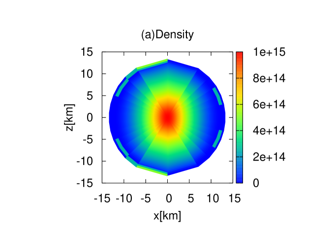
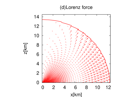
Figure 1.— Distribution of the rest mass density, the magnetic field, the magnetic pressure ratio to matter pressure, the Lorenz force, and the adiabatic index for the non-rotating star with SLy EOS. (a) Equi-density contours, (b) equi-$P_{\rm mag}/P_{\rm matter}$ contours, (c) equi-$B_{(\phi)}$ contours, (d) the Lorenz force, and (e) adiabatic index on the meridional plane for the $M=1.41M_{\odot}$, $B_{\rm max}=7.8\times 10^{17}$G, $R_{\rm cir}=14.4$[km], and $H/|W|=0.187$ model. In the panel (a)-(c), the solid lines correspond to the stellar surface. In the panel of (d), the thick lines represents the surface.

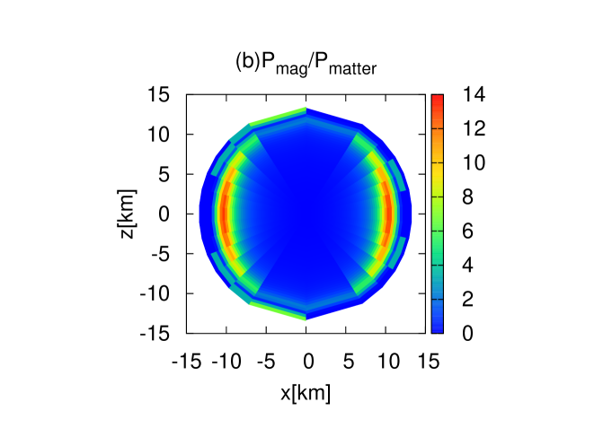
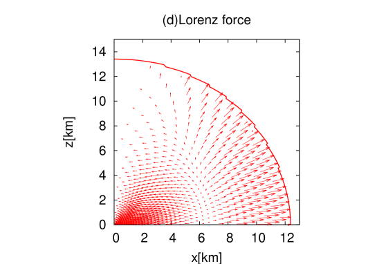
Figure 2.— Same as Fig. 1, but for FPS EOS, the $M=1.1M_{\odot}$, $B_{\rm max}=6.9\times 10^{17}$G, $R_{\rm cir}=14.2$[km], and $H/|W|=0.193$ model.

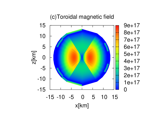
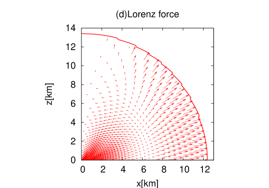
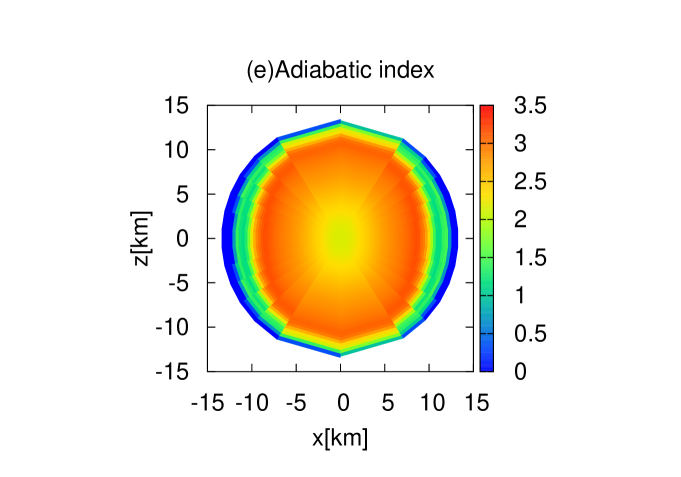
Figure 3.— Same as Fig. 1, but for Shen EOS, the $M=2.3M_{\odot}$, $B_{\rm max}=8.2\times 10^{17}$G, $R_{\rm cir}=15.8$[km], and $H/|W|=0.148$ model.

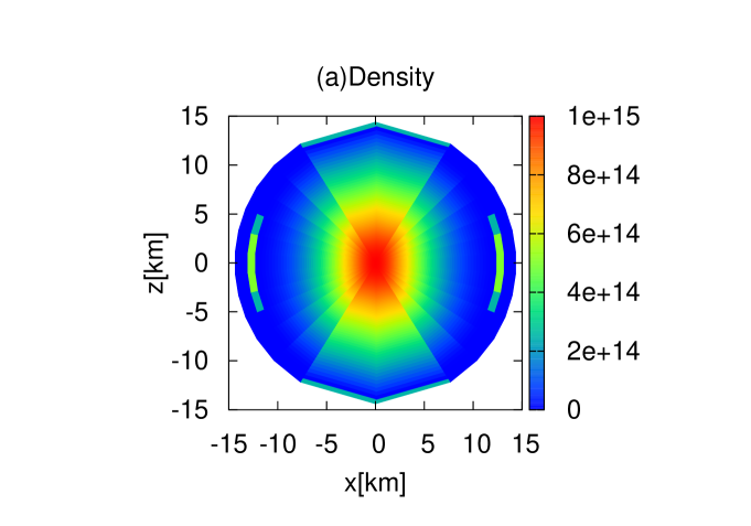
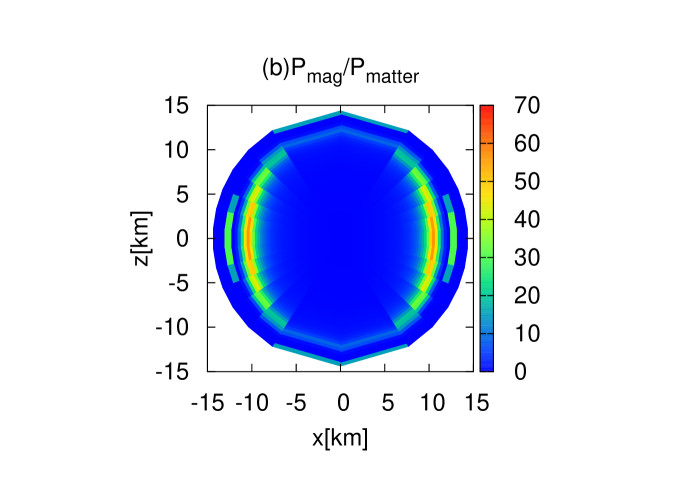
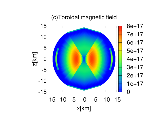
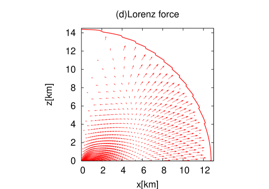
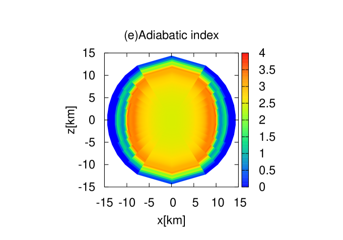
Figure 4.— Same as Fig. 1, but for LS EOS, the $M=1.56M_{\odot}$, $B_{\rm max}=7.36\times 10^{17}$G, $R_{\rm cir}=14.9$[km], and $H/|W|=0.173$ model.

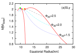
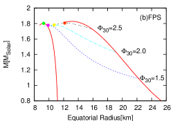
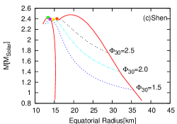
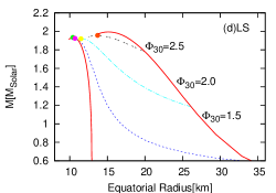
Figure 5.— Circumferential radius versus gravitational mass for models with (a) SLy, (b) FPS, (c) Shen, and (d) LS EOS. The left thick line represents spherical, non-magnetized configurations, and the right thick line represents the boundary beyond which converged solution could not be obtained. Along the dotted lines labeled with $\Phi_{30}$, the configurations have constant magnetic flux, and $\Phi_{30}$ denotes the flux value normalized by $10^{22}{\rm G~{}cm^{2}}$. The filled circles indicate the maximum gravitational mass models whose global physical quantities are given in Table 1.

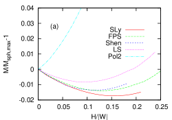
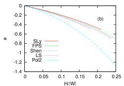
Figure 6.— Dependence of (a) maximum gravitational mass and (b) mean deformation rate on the ratio of the magnetic energy $H$ to the gravitational biding energy $W$. $M_{\rm sph,max}$ denotes the maximum mass of the spherical stars for each realistic EOS. As a reference, the relation under the polytropic EOS is shown as Pol2, where the polytropic index is set to be unity.

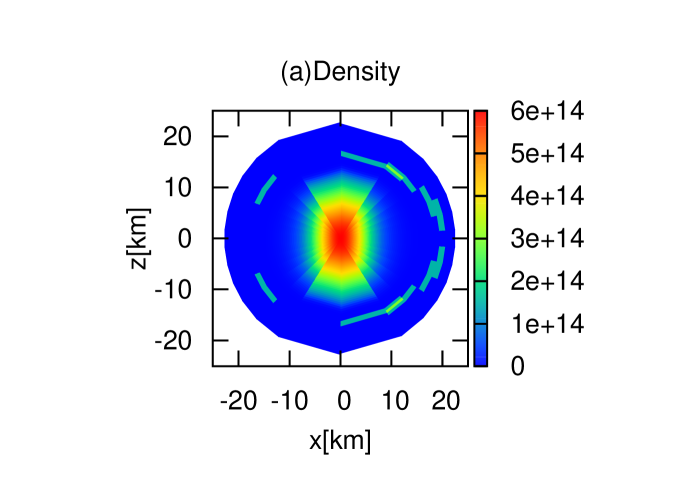
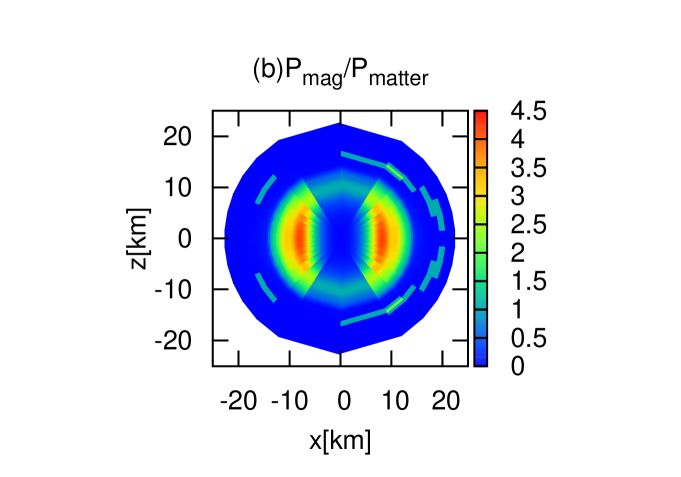
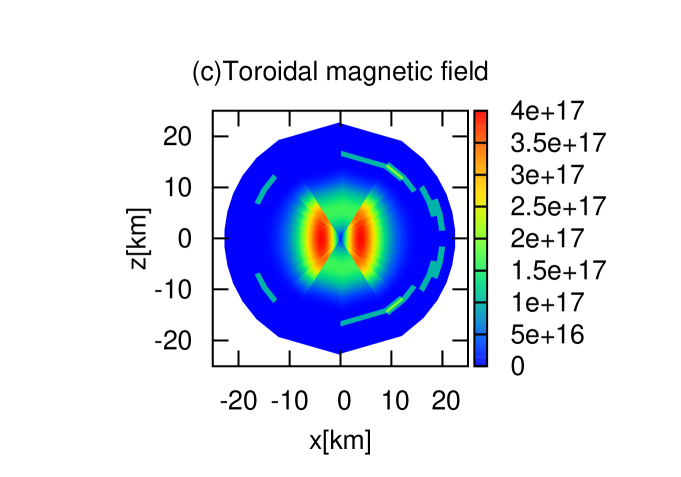
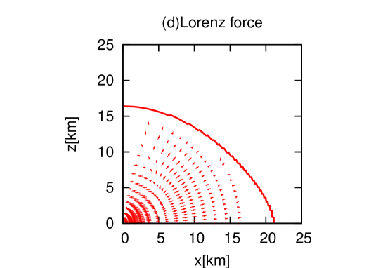
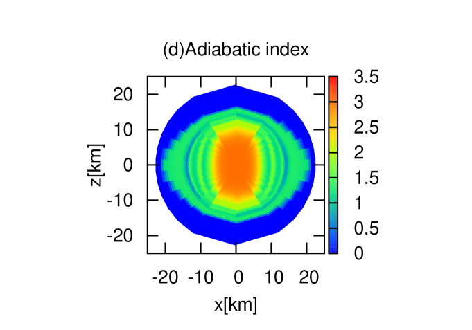
Figure 7.— Distribution of the rest mass density, the magnetic field, the magnetic pressure ratio to matter pressure, the Lorenz force, and the adiabatic index for the rotating star with SLy EOS. (a) Equi-density contours, (b) equi-$P_{\rm mag}/P_{\rm matter}$ contours, (c) equi-$B_{(\phi)}$ contours, (d) the Lorenz force, and (e) adiabatic index on the meridional plane for the $M=2.00M_{\odot}$, $B_{\rm max}=5.49\times 10^{17}$G, $R_{\rm cir}=25.0$[km], $\Omega_{3}=1.87$, and $H/|W|=0.152$ model. In the panel (a)-(c), the solid lines correspond to the stellar surface. In the panel of (d), the thick lines represents the surface.

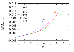
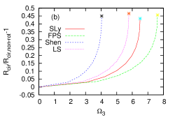
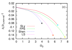
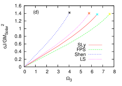
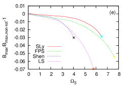
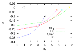
Figure 8.— Global physical quantities $M$, $R_{\rm cir}$, $\rho_{c}$, $J$, $B_{\rm max}$, and $\bar{e}$ for the constant baryon mass and magnetic flux equilibrium sequences with the several realistic EOSs, given as functions of $\Omega$. The solid, dashed, long-dashed , and dotted lines represent the sequences with SLy, FPS, Shen, LS EOS, respectively. All the plots show the increasing (decreasing) rates of the global quantities from those for the non-rotating limits. All the equilibrium sequences are referred to the normal equilibrium sequences characterized by the constant baryon rest mass $M_{0}=1.90M_{\odot}$ and the constant magnetic flux $\Phi_{30}=1.0$. The asterisks indicate the mass-shedding models.

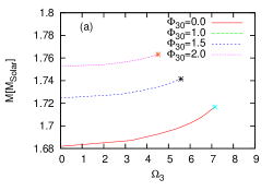
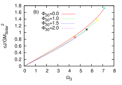
Figure 9.— Global physical quantities $M$ and $J$ for the constant baryon mass and magnetic flux equilibrium sequences with SLy EOS, given as functions of $\Omega$. Results for the $M_{0}=1.9M_{\odot}$ models with $\Phi_{30}=0$, $1$, $1.5$, and $2$ are shown. The solid, dashed, long-dashed, and dotted lines correspond to the equilibrium sequences characterized by $\Phi_{30}=0$, $1$, $1.5$, and $2$, respectively.

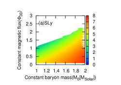
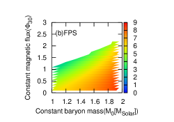
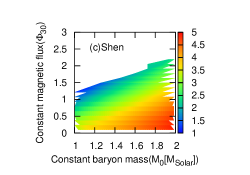
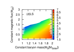
Figure 10.— Equi-$\Omega_{\rm ms}$ contours on $M_{0}$-$\Phi$ plane for (a) SLy, (b) FPS, (c) Shen, and (d) LS EOS. The white regions which lies on the left-upper sides of the panels represent the non-converged limits.

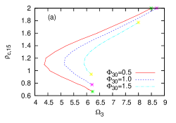
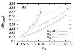
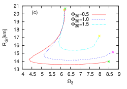
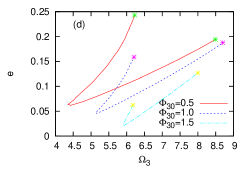
Figure 11.— Global quantities, $\rho_{c}$, $\bar{e}$, $M$, and $R_{\rm cir}$ along the supramassive sequence with Shen EOS which is characterized by the constant baryon rest mass $M_{0}=2.90M_{\odot}$. The solid, dashed, and long-dashed lines correspond to the sequences with $\Phi_{30}=0.5$, $1.0$, $1.5$, respectively.

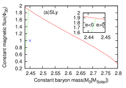
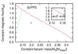
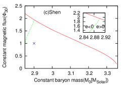
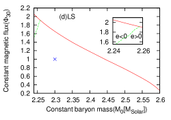
Figure 12.— Phase diagram on constant baryon mass and magnetic flux plane of the supramassive sequences for (a)SLy, (b) FPS, (c) Shen, and (d) LS EOS. The solid lines correspond to the critical line, above which there exists no physical solution (see the text for details). The dashed lines show the models with $\bar{e}=0$. In the left (right) side regions of the dotted lines, the supramassive sequences have the prolate (oblate) solutions. The magnified panels are put on the upper right of the each figures. The cross symbols in each panel represent the sequences given in Table 4 (see the text for details).

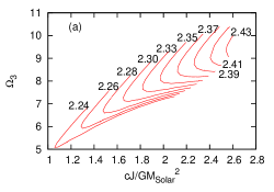
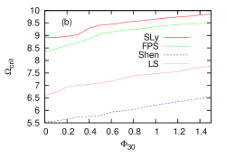
Figure 13.— (a) Angular momentum and angular velocity relation in the supramassive sequences with LS EOS and $\Phi_{30}=1.0$. The numbers attached on the each sequences represent the values of constant baryon rest mass in units of $M_{\odot}$. (b) Critical spin up angular velocity as functions of the magnetic flux for each EOS. The critical angular velocity is defined by the value from which the stars start to spin up (see the text in details).

References

- Akiyama et al. (2003) Akiyama, S., Wheeler, J. C., Meier, D. L., & Lichtenstadt, I. 2003, APJ, 584, 954
- Akmal & Pahdharipahde (1998) Akmal, A., Pandharipande, V. R., & Ravenhall, D. G. 1998, PRC, 58, 1804
- Balbus & Hawley (1991) Balbus, S. A. & Hawley, J. F. 1991, APJ, 376, 214
- Baym & Pethick (1979) Baym, G., & Pethick, C. 1979, Ann. Rev. Astron. Astrophys., 17, 415
- Boucquet et al. (1995) Bocquet, M., Bonazzola, S., Gourgoulhon, E., & Novak, J. 1995, A&A, 301, 757
- Bonazzola & Gourgoulhon (1994) Bonazzola, S. & Gourgoulhon, E. 1994, CQG, 11, 1775
- Bonazzola & Gourgoulhon (1996) Bonazzola, S., & Gourgoulhon, E. 1996, A&A 312, 675
- Bonazzola et al. (1998) Bonazzola, S., Gourgoulhon, E., & Marck, J.-A. 1998, Phys. Rev. D, 58, 104020
- Braithwaite & Spruit (2004) Braithwaite, J. and Spruit, H. C., 2004, Nature 431, 819
- Broderick et al. (2000) Broderick, A., Prakash, M., & Lattimer, J. M. 2000, ApJ, 537, 351
- Cardall et al. (2001) Cardall, C. Y., Prakash, M., & Lattimer, J. M. 2001, ApJ, 554, 322
- Carter (1969) Carter, B. 1969, J. Math. Phys. 10, 70
- Chandrasekhar & Fermi (1953) Chandrasekhar, S., & Fermi, E. 1953, ApJ 118, 116
- Cook et al. (1992) Cook, G. B., Shapiro,S. L. & Teukolsky, S. A., 1992, ApJ 398, 203, 1994, APJ 422, 227
- Cutler (2002) Cutler, C. 2002, PRD 66, 084025
- Dessart et al. (2007) Dessart, L., Burrows, A., Livne, E., & Ott, C. D. 2007, APJ, 669, 585
- Douchin & Haensel (2001) Douchin, F., & Haensel, P. 2001, A&A, 380, 151
- Ferrario & Wickramasinghe (2006) Ferrario, L. & Wickramasinghe, D. 2006, MNRAS, 367, 1323
- Friedman & Pandharipande (1981) Friedman, B., & Pandharipande, V. R. 1981, Nuclear Physics A, 361, 502
- Friedman et al. (1988) Friedman, J. L., Ipser, J. R., & Sorkin, R. D., 1988, Apj 325, 722
- Geppert & Rheinhardt (2006) Geppert, U. & Rheinhardt, M. 2006, A& A, 456, 639
- Glendenning (2001) Glendenning, N. K. 2001, Physics. Rep., 342, 393
- Goldreich & Julian (1969) Goldreich, P. & Julian, W., 1969, APJ, 238, 991
- Goldreich & Reisenegger (1992) Goldreich, P. & Reisenegger, A., 1992, APJ, 395, 250
- Gourgoulhon & Bonazzola (1993) Gourgoulhon, E., & Bonazzola, S. 1993, PRD, 48, 2635
- Gourgoulhon & Bonazzola (1994) Gourgoulhon, E., & Bonazzola, S. 1994 CQG, 11, 443
- Harding & Lai (2006) Harding, A. K., & Lai, D. 2006, Reports of Progress in Physics, 69, 2631
- Heger et al. (2005) Heger, A., Woosley, S. E., and Spruit, H. C., 2005, APJ 626, 350
- Hachisu (1986) Hachisu, I. 1986, ApJS, 61, 479
- Ioka & Sasaki (2003) Ioka, K. & Sasaki, M. 2003, PRD 67, 124026
- Ioka & Sasaki (2004) Ioka, K. & Sasaki, M. 2004, ApJ 600, 296
- Kiuchi & Kotake (2008) Kiuchi, K., & Kotake, K. 2008, MNRAS 385, 1327
- Kiuchi & Yoshida (2008) Kiuchi, K. & Yoshida, S. 2008, PRD 78, 044045
- Kiuchi et al. (2008) Kiuchi, K., Shibata, M. & Yoshida, S., 2008, PRD 78, 024029
- Komatsu et al. (1989) Komatsu, H., Eriguchi, Y., & Hachisu, I., MNRAS, 237, 355 (1989), 239, 153 (1989)
- Konno et al. (1999) Konno, K., Obata, T.& Kojima, Y. 1999, A&A, 352, 211
- Kotake et al. (2004) Kotake, K., Sawai, H., Yamada, S., & Sato, K. 2004, ApJ, 608, 391
- Kotake et al. (2006) Kotake, K., Sato, K., & Takahashi, K. 2006, Reports of Progress in Physics, 69, 971
- Kouveliotou (1998) Kouveliotou, C., et al. 1998, Nature, 393, 235
- Lattimer & Prakash (2007) Lattimer, J. M. & Prakash, M. 2007 Phys. Rept. 442, 109
- Lattimer & Swesty (1991) Lattimer, J. M., & Douglas Swesty, F. 1991, Nuclear Physics A, 535, 331
- Livne et al. (2007) Livne, E., Dessart, L., Burrows, A., & Meakin, C. A. 2007, ApJS, 170, 187
- Lyne & Graham-Smith (2005) Lyne A. & Graham-Smith, F. Pulsar Astronomy (Cambridge University Press, 2005).
- Miketinac (1973) Miketinac, M. J. 1973 Ap&SS, 22, 413
- Morrison et al. (2004) Morrison, I. A., Baumgarte, T. W., & Shapiro, S. L. 2004, ApJ, 610, 941
- Nozawa et al. (1998) Nozawa, T., Stergioulas, N., Gourgoulhon, E., & Eriguchi, Y. 1998, A&A Sup. Ser., 132, 431
- Obergaulinger et al. (2006) Obergaulinger, M., Aloy, M. A., Müller, E. 2006, A&A, 450, 1107
- Oron (2002) Oron, A., 2002, PRD, 66, 023006
- Pons & Geppert (2007) Pons, J. A., & Geppert, U. 2007, A&A, 470, 303
- Pandharipande & Ravenhall (1989) Pandharipande, V. R., & Ravenhall, D. G. 1989, NATO ASIB Proc. 205: Nuclear Matter & Heavy Ion Collisions, 103
- Reisenegger (2001) Reisenegger, A. 2001, ApJ, 550, 860
- Reisenegger (2008) Reisenegger, A., arXiv:0809.0361 [astro-ph]
- Sawai et al. (2008) Sawai, H., Kotake, K., & Yamada, S. 2008, APJ, 672, 465
- Shapiro & Teukolsky (1983) Shapiro, S. L., & Teukolsky, S. A. 1983, Research supported by the National Science Foundation. New York, Wiley-Interscience, 1983, 645 p.,
- Shapiro et al. (1990) Shapiro, S. L., Teukolsky, S.A., & Nakamura, T. 1990, ApJ, 357, L17
- Shen et al. (1998a) Shen, H., Toki, H., Oyamatsu, K., Sumiyoshi, K. 1998a, Nuclear Physics, A637, 435, 109, 301
- Shen et al. (1998b) Shen, H., Toki, H., Oyamatsu, K., & Sumiyoshi, K. 1998b, Progress of Theoretical Physics, 100, 1013
- Shibata et al. (2005) Shibata, M., Taniguchi, K., & Uryu, K., 2005, PRD 71, 084021
- Shibata et al. (2006) Shibata, M., Liu, Y. T., Shapiro, S. L., & Stephens, B. C. 2006 PRD 74, 104026
- Spruit (2007) Spruit, H. C. astro-ph/0711.3650.
- Sumiyoshi et al. (2005) Sumiyoshi, K., Yamada, S., Suzuki, H., Shen, H., Chiba, S., & Toki, H. 2005, ApJ, 629, 922
- Takiwaki et al. (2004) Takiwaki, T., Kotake, K., Nagataki, S., & Sato, K. 2004, ApJ, 616, 1086
- Takiwaki et al. (2009) Takiwaki, T., Kotake, K., & Sato, K. 2009, ApJ, 691, 1360
- Tayler (1973) Tayler, R. J., 1973 MNRAS, 161, 365
- Thompson & Duncan (1993) Thompson, C. & Duncan, R. C. 1993, ApJ, 408, 194
- Thompson & Duncan (1995) Thompson, C. & Duncan, R. C. 1995, MNRAS, 275, 255
- Thompson & Duncan (1996) Thompson, C. & Duncan, R. C. 1996, ApJ 473, 322
- Tomimura & Eriguchi (2005) Tomiumra, Y. & Eriguchi, Y. 2005 MNRAS, 359, 1117
- Trehan & Uberoi (1972) Trehan, S. K. & Uberoi, M. S. 1972 ApJ, 175, 161
- Wald (1984) Wald, R. M. 1984, General Relativity (The University of Chicago Press),
- Watts (2006) Watts, A. 2006, 36th COSPAR Scientific Assembly, 36, 168
- Wiringa et al. (1988) Wiringa, R. B., Fiks, V., & Fabrocini, A. 1988, PRC, 38, 1010
- Woods & Thompson (2004) Woods, P. M. & Thompson, C. 2004, arXiv:astro-ph/0406133.
- Yoshida & Eriguchi (2006) Yoshida, S. & Eriguchi, Y. 2006, ApJS, 164, 156
- Yoshida et al. (2006) Yoshida, S., Yoshida, S., & Eriguchi, Y. 2006, ApJ, 651, 462