Glossary

• Extrinsic effect an effect which has an explicit dependence on the form or strength of the disorder potential.

• Intrinsic effect an effect which does not depend explicitly on the form and strength of the disorder potential.

• Semiclassical theory a theory in which a particle’s position and momentum are considered simultaneously.

• Spin-orbit interaction a relativistic interaction between the spin of a particle and its momentum (which is associated with its orbital motion.)

• Steady-state spin current a flow of spins induced by an electric field.

• Steady-state spin density a net spin density induced by an electric field.

1 Definition of the subject and its importance

Spin transport refers to the physical movement of spins across a sample and, if spin were a conserved quantity, one could make a straightforward distinction between spin-up and spin-down charge currents. The recent upsurge of interest in spin transport is, however, motivated by systems in which spin is not conserved due to the presence of spin-orbit interactions, which give rise to spin precession. Here, due to non-conservation of spin the spin current is not well defined [1, 2, 3]. Spin transport in these cases usually does not involve charge transport as the charge currents in the direction of spin flow cancel out. Finally, in certain materials, spin currents are accompanied by steady-state spin densities. The appearance of a spin density is not a transport phenomenon, but it is a steady-state process and is intimately connected to spin transport.

The word semiclassical as used in this work refers to theories which consider the position and momentum of a particle simultaneously. Semiclassical pictures are intuitive and useful in descriptions of transport, particularly in inhomogeneous systems and in spatially dependent fields, which typically vary on length scales much larger than atomic size.

In recent years, steady progress has been made towards realization of convenient semiconducting ferromagnets and spin injection into semiconductors from ferromagnetic metals [4, 5, 6, 7] yet spin injection from a ferromagnetic metal into a semiconductor is hampered by the resistivity mismatch between the two [8]. This is one factor, in addition to basic science, motivating the search for an understanding of the way spins are manipulated electrically. The last few years have seen many experimental advances in spin transport, and spin currents have been measured directly [9, 10] and indirectly [11, 12, 13, 14, 15].

2 Introduction

Novel physical phenomena that may lead to improved memory devices and advances in quantum information processing are closely related to spin-orbit interactions. [16] Spin-orbit interactions are present in the band structure and in potentials due to impurity distributions. Spin-orbit coupling is in principle always present in impurity potentials and gives rise to skew scattering. Band structure spin-orbit coupling may arise from the inversion asymmetry of the underlying crystal lattice [17] (bulk inversion asymmetry), from the inversion asymmetry of the confining potential in two dimensions [18] (structure inversion asymmetry), and may be present also in inversion symmetric systems. [19]

Although many observations in this entry are general, the discussion will focus on non-interacting spin-1/2 electron systems, which are pedagogically easier. The Hamiltonian of these systems typically contains a kinetic energy term and a spin-orbit coupling term, $H_{{\bm{k}}}=\frac{\hbar^{2}k^{2}}{2m^{*}}+H_{{\bm{k}}}^{\mathrm{so}}$, where $m^{*}$ is the electron effective mass. In spin-1/2 electron systems, band structure spin-orbit coupling can always be represented as a Zeeman-like interaction of the spin with a wave vector-dependent effective magnetic field ${\bm{\Omega}}_{\bm{k}}$, thus $H_{{\bm{k}}}^{\mathrm{so}}=(1/2)\,{\bm{\sigma}}\cdot{\bm{\Omega}}_{\bm{k}}$. Common examples of effective fields are the Rashba spin-orbit interaction, [18] which is often dominant in quantum wells with inversion asymmetry, and the Dresselhaus spin-orbit interaction, [17] which is due to bulk inversion asymmetry. The spin operator is given by $s^{\sigma}=(\hbar/2)\,\sigma^{\sigma}$, where $\sigma^{\sigma}$ is a Pauli spin matrix. The spin current operator in these systems will be taken to be $\hat{\mathcal{J}}^{\sigma}_{i}=(1/2)\,\{s^{\sigma},v^{i}\}$, where the velocity operator is $v^{i}=(1/\hbar)\,\partial H_{\bm{k}}/\partial k_{i}$.

An electron spin at wave vector ${\bm{k}}$ precesses about the effective field ${\bm{\Omega}}_{\bm{k}}$ with frequency $\Omega_{\bm{k}}/\hbar\equiv|{\bm{\Omega}_{\bm{k}}}|/\hbar$ and is scattered to a different wave vector within a characteristic momentum scattering time $\tau_{p}$. I will assume in this work that $\varepsilon_{F}\tau_{p}/\hbar\gg 1$, where $\varepsilon_{F}$ is the Fermi energy, which is equivalent to the assumption that the carrier mean free path is much larger that the de Broglie wavelength. Within this range, the relative magnitude of the spin precession frequency $\Omega_{\bm{k}}$ and inverse scattering time $1/\tau_{p}$ define three qualitatively different regimes. In the ballistic (clean) regime no scattering occurs and the temperature tends to absolute zero, so that $\varepsilon_{F}\tau_{p}\rightarrow\infty$ and $\Omega_{\bm{k}}\tau_{p}/\hbar\rightarrow\infty$. The weak scattering regime is characterized by fast spin precession and little momentum scattering due to, e.g., a slight increase in temperature, yielding $\varepsilon_{F}\tau_{p}/\hbar\gg\Omega_{\bm{k}}\,\tau_{p}/\hbar\gg 1$. In the strong momentum scattering regime $\varepsilon_{F}\tau_{p}/\hbar\gg 1\gg\Omega_{\bm{k}}\,\tau_{p}/\hbar$. I will concentrate on effects originating in the band structure, the observation of which requires the assumption that the materials under study are in the weak momentum scattering regime. Electric fields will be assumed uniform.

The first part of this article will present a semiclassical theory of spin transport, identifying the terms responsible for spin currents in the microscopic dynamics of carriers. Spin non-conservation as a result of spin precession leads to several possible definitions of the spin current, which emerge out of the spin equation of continuity. The second part presents a different point of view, which explains aspects not easily captured in the semiclassical approach. The steady-state density matrix is shown to contain a contribution due to precessing spins and one due to conserved spins. Steady state corrections $\propto\tau_{p}$ are associated with the absence of spin precession and give rise to spin densities in external fields. [20, 21, 22, 23, 24, 26, 25, 27, 28] Steady state corrections independent of $\tau_{p}$ are associated with spin precession and give rise to spin currents in external fields. [1, 2, 3, 9, 10, 11, 12, 13, 14, 15, 29, 30, 31, 32, 33, 34, 35, 36, 37, 38, 39, 40, 41, 42, 43, 44, 45, 46] Scattering between these two distributions induces significant corrections to steady-state spin currents.

3 Spin currents in electric fields

3.1 Wave-packet picture of spin transport

This section presents a semiclassical theory of spin transport valid for a general spin-orbit system. The semiclassical method is a suitable approach to the study of transport, because, typically, in the relevant systems the external fields vary smoothly on atomic length scales. All information about the system is taken to be contained in the band structure, thus allowing a description of spin transport which does not make reference to the detailed form of the spin-orbit interaction.

The system under study is regarded as as a collection of carriers, whose semiclassical dynamics in a non-degenerate band $i$ are described by a wave packet [47], with its charge centroid having coordinates (${\bf r}_{c},{\bf k}_{c}$)

$$|w_{i}\rangle=\int d^{3}k\;a({\bf k},t)e^{i{\bf k}\cdot\hat{\bf r}}|u_{i}({\bf r}_{c},{\bf k},t)\rangle.$$ (1)

In the above, the function $a({\bf k},t)$ is a narrow distribution sharply peaked at ${\bf k}_{c}$, the phase of which specifies the center of charge position ${\bf r}_{c}$, while $|u_{i}({\bf r}_{c},{\bf k},t)\rangle$ are lattice-periodic Bloch wave functions. The size of the wave packet in momentum space must be considerably smaller than that of the Brillouin zone. In real space, this implies that the wave packet must stretch over many unit cells.

The external electric field drives the center of the wave packet in $k$-space according to the semiclassical equations of motion

$$\hbar\dot{\bf r}_{c}=\frac{\partial\varepsilon_{i}}{\partial{\bf k}_{c}}-q{\bf E}\times{\bf\Omega}_{i}$$ (2)

$$\hbar\dot{\bf k}_{c}=q{\bf E},$$

with $q$ the charge of the carriers, $\varepsilon_{i}$ the band energy, and the Berry curvature

$${\bf\Omega}_{i}=i\langle\frac{\partial u_{i}}{\partial{\bf k}}|\times|\frac{\partial u_{i}}{\partial{\bf k}}\rangle.$$ (3)

The electric field also gives rise to an adiabatic correction to the wave functions, which mixes the states making up the wave packet. The wave functions $|u_{i}\rangle$ therefore have the following form:

$$|u_{i}\rangle=|\phi_{i}\rangle-\sum_{j}\frac{\langle\phi_{j}|i\hbar\frac{d}{dt}|\phi_{i}\rangle}{\varepsilon_{i}-\varepsilon_{j}}|\phi_{j}\rangle,$$ (4)

where the $\phi_{i}$ are the unperturbed Bloch eigenstates. The $|u_{i}\rangle$ form a complete set and retain the Bloch periodicity.

The distribution of carriers is described by a function $f$. When scattering is present, the distribution function satisfies the following equation:

$$\frac{\partial f}{\partial t}+\dot{\bf r}_{c}\cdot\frac{\partial f}{\partial{\bf r}_{c}}+\dot{\bf k}_{c}\cdot\frac{\partial f}{\partial{\bf k}_{c}}=\bigg{(}\frac{df}{dt}\bigg{)}_{coll},$$ (5)

where $(\frac{df}{dt})_{coll}$ is the usual collision term. In independent bands, in the relaxation time approximation, the collision term takes the form $\frac{f_{0}-f}{\tau_{p}}$, with $f_{0}$ the equilibrium distribution and $\tau_{p}$ the momentum relaxation time. In the Boltzmann theory, the change in the distribution function with time arises through the drift terms, which are determined from the semiclassical equations of motion, as well as through scattering with other carriers, with localized impurities or with phonons. For transport in a non-degenerate band, it is consistent to ignore interband scattering effects in the weak scattering limit. In this case the relaxation time is a scalar quantity. The effects of interband coherence due to scattering will be explored in the next section.

In order to obtain expressions for macroscopic quantities of interest, such as densities and currents, one needs to carry out a coarse graining by averaging over microscopic fluctuations. In classical dynamics this coarse graining is performed by means of a sampling function, which is smooth and has a significant magnitude only in a finite range [48]. This range is large compared to atomic dimensions, but small compared to the scale of variation of the distribution function. Moreover, it has a rapidly converging Taylor expansion over distances of atomic dimensions, and its form does not need to be specified. This method has a close analog in wavepacket dynamics, where the sampling function is replaced by a $\delta$-function.

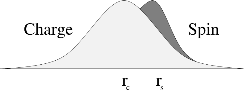
Figure 1: For a particle of finite extent the charge and spin distributions in real space are in general do not coincide. The same is true of the charge and spin distributions in reciprocal space.

It is crucial to recognize that, in general, the center of spin and the center of charge are distinct, since the wave packet samples a range of wave vectors and the spin is usually a function of k. Following the line of thought outlined above, the spin density is defined to be (henceforth ${\bf k}_{c}$ will be abbreviated to k)

$$S^{\sigma}({\bf R},t)=\int\!\int d^{3}kd^{3}r_{c}f({\bf r}_{c},{\bf k},t)\langle\delta({\bf R}-{\bf\hat{r}})\hat{s}^{\sigma}\rangle,$$ (6)

where the bracket indicates quantum mechanical averaging over the wave packet with charge centroid $({\bf r}_{c},{\bf k})$. As the $\delta$-function has operator arguments, it will be regarded as a sampling operator, whose expectation value yields a spatial average, evaluated at position r. To account for the fact that spin is not conserved, a new quantity is introduced, which will be referred to as the torque density, defined by

$${\cal T}^{\sigma}({\bf R},t)=\int\!\int d^{3}kd^{3}r_{c}f({\bf r}_{c},{\bf k},t)\langle\delta({\bf R}-{\bf\hat{r}})\hat{\tau}^{\sigma}\rangle.$$ (7)

$\hat{\tau}^{\sigma}$ in the above stands for the rate of change of the spin operator, given by $\frac{i}{\hbar}[\hat{H},\hat{s}^{\sigma}]$, and symmetrization of products of non-commuting operators has been assumed. Finally, the microscopic spin current density is defined as:

$$\bm{\mathcal{J}}^{\sigma}({\bf R},t)=\int\!\int d^{3}kd^{3}r_{c}f({\bf r}_{c},{\bf k},t)\langle\delta({\bf R}-{\hat{\bf r}}){\hat{s}^{\sigma}{\hat{\bf v}}}\rangle.$$ (8)

We obtain the following continuity equation for the spin density and current:

$$\frac{\partial S^{\sigma}}{\partial t}+\nabla\cdot\bm{\mathcal{J}}^{\sigma}={\cal T}^{\sigma}+{\cal F}^{\sigma}.$$ (9)

The equation of continuity contains a bulk source term, which coincides with the torque density and acts as a mechanism for spin generation. Similar source terms are associated with nonconserved quantities, for example, in quantum electrodynamics and in Maxwell’s equations. The last term in (9) represents the scattering contribution, which will be discussed further below.

Figure 2: In the presence of spin-orbit interactions the spin distribution of a particle changes in time. The horizontal axis may represent position or wave vector.

Let us discuss the terms in the equation of continuity, beginning with the spin density. The argument of the sampling operator can be expressed as $[{\bf r}-{\bf r}_{c}-(\hat{\bf r}-{\bf r}_{c})]$, and, as the second term is of atomic dimensions, the sampling operator can be written as a Taylor expansion about $(\hat{\bf r}-{\bf r}_{c})$. The density can therefore be re-expressed, in terms of macroscopic quantities, as

$$S^{\sigma}({\bf R},t)=\rho^{s\sigma}({\bf R},t)-\nabla_{\bf R}\cdot{\bf P}^{s\sigma}({\bf R},t),$$ (10)

where summation over repeated indices has been assumed. In the above, the monopole density is given by

$$\rho^{s\sigma}({\bf R},t)=\int\!\int d^{3}kd^{3}r_{c}f({\bf r}_{c},{\bf k},t)\langle\hat{s}^{\sigma}\rangle\delta({\bf R}-{\bf r}_{c})=\int d^{3}kf\langle\hat{s}^{\sigma}\rangle|_{{\bf r}_{c}={\bf R}},$$ (11)

where $f$ in the second line, and henceforth, is to be understood as $f({\bf R},{\bf k},t)$, and the dipole density is

$${\bf P}^{s\sigma}({\bf R},t)=\int\!\int d^{3}kd^{3}r_{c}f\langle(\hat{\bf r}-{\bf r}_{c}){\hat{s}^{\sigma}}\rangle\delta({\bf R}-{\bf r}_{c})=\int d^{3}kf{\bf p}^{s\sigma}|_{{\bf r}_{c}={\bf R}}.$$ (12)

The average spin of the wave packet has been denoted by $\langle\hat{s}^{\sigma}\rangle$, and the spin-dipole is defined to be ${\bf p}^{s\sigma}=\langle(\hat{\bf r}-{\bf r}_{c})\hat{s}^{\sigma}\rangle|_{{\bf r}_{c}={\bf R}}$. It will be seen that the first term in the density is the average of a monopole density located at ${\bf r}_{c}$, while the dipole term is the average of a point dipole density located at ${\bf r}_{c}$, and similarly for higher orders. The dipole must be understood as the average of the quantum mechanical dipole operator, as an exact analogy with the electric dipole of classical electrodynamics cannot be made. The density can thus be viewed as a collection of point multipoles, located at the centroid of each wave packet. The microscopic distribution of spin is important at the molecular level, but at the macroscopic level the effect of this molecular distribution is replaced by a sum of multipoles. Since the center of spin is different from the center of charge, in principle all multipoles are present.

Following a similar manipulation and using the Boltzmann equation, the torque density is re-expressed as:

$${\cal T}^{\sigma}({\bf R},t)=\rho^{\tau\sigma}({\bf R},t)-\nabla\cdot{\bf P}^{\tau\sigma}({\bf R},t)$$ (13)

with the torque monopole density

$$\rho^{\tau\sigma}({\bf R},t)=\int\!\int d^{3}kd^{3}r_{c}f({\bf r}_{c},{\bf k},t)\langle\hat{\tau}^{\sigma}\rangle\delta({\bf R}-{\bf r}_{c})=\int d^{3}kf\langle\hat{\tau}^{\sigma}\rangle|_{{\bf r}_{c}={\bf R}},$$ (14)

and the torque dipole density

$${\bf P}^{\tau\sigma}({\bf R},t)=\int\!\int d^{3}kd^{3}r_{c}f({\bf r}_{c},{\bf k},t)\langle({\bf\hat{R}}-{\bf r}_{c})\hat{\tau}^{\sigma}\rangle|_{{\bf r}_{c}={\bf R}}=\int d^{3}kf{\bf p}^{\tau\sigma}|_{{\bf r}_{c}={\bf R}}.$$ (15)

In analogy with the spin dipole, the torque dipole has been defined as ${\bf p}^{\tau\sigma}=\langle(\hat{\bf r}-{\bf r}_{c})\hat{\tau}^{\sigma}\rangle|_{{\bf r}_{c}={\bf R}}$. The torque density is therefore also a sum of multipole moments, that is, the moments of a point spin source located at ${\bf r}_{c}$. Even in the case when the center of $\langle\hat{s}^{\sigma}\rangle$ coincides with the center of charge, $\langle\hat{\tau}^{\sigma}\rangle$ may not be centered at ${\bf r}_{c}$, with the result that the higher order terms in the torque density are in general present. The second and higher terms of ${\cal T}^{\sigma}$ cancel exactly the analogous terms in the continuity equation which come from the current.

Since only the gradient of the spin current appears in the equation of continuity, in the expansion of the sampling operator we keep the leading term

$$\bm{\mathcal{J}}^{s}({\bf R},t)=\int d^{3}kf\langle{\hat{\bf v}}\hat{s}^{\sigma}\rangle|_{{\bf r}_{c}={\bf R}}.$$ (16)

Keeping terms to first order in $({\bf\hat{r}}-{\bf r}_{c})$, the current can be decomposed into the following:

$$\bm{\mathcal{J}}^{s\sigma}={\bf C}^{s\sigma}+{\bf D}^{s\sigma}-{\bf P}^{\tau\sigma}$$ (17)

The convective term ${\bf C}^{s\sigma}$ represents the spin being transported along with the wave packet

$${\bf C}^{s\sigma}({\bf R},t)=\int\!\int d^{3}kd^{3}r_{c}f({\bf r}_{c},{\bf k},t){\bf\dot{r}}_{c}\langle\hat{s}^{\sigma}\rangle\delta({\bf R}-{\bf r}_{c})=\int d^{3}kf{\bf c}^{s\sigma}|_{{\bf r}_{c}={\bf R}},$$ (18)

while ${\bf D}^{s\sigma}$ comes from the rate of change of the spin dipole, which has already been introduced. It has the form:

$${\bf D}^{s\sigma}({\bf R},t)=\int d^{3}kf\frac{d{\bf p}^{s\sigma}}{dt}|_{{\bf r}_{c}={\bf R}}$$ (19)

${\bf P}^{\tau\sigma}$ is the torque dipole introduced above. The corresponding monopole term appears in the source term of the continuity equation, as will emerge below. The presence of the torque dipole here is to be contrasted with the absence of an analogous term in classical electrodynamics. There, an electric dipole arises from the placement of two charges a small distance from each other, but the charge itself is conserved.

Finally, we come to the source term in (9). The first part, composed of the torque density, has already been discussed. The second term, denoted by ${\cal F}^{\sigma}$, becomes, in the relaxation time approximation

$${\cal F}^{\sigma}=\frac{S^{\sigma}_{0}-S^{\sigma}}{\tau_{p}}=\frac{1}{\tau_{p}}\int d^{3}k(f_{0}-f)\langle\hat{s}^{\sigma}\rangle,$$ (20)

where $\tau_{p}$ is the momentum relaxation time and $f_{0}$ the equilibrium distribution, which is usually the Fermi-Dirac distribution function.

Based on the continuity equation alone, there is some flexibility in defining the current and the source. In systems in which spin is conserved, the torque density becomes, to first order in $({\bf\hat{r}}-{\bf r}_{c})$, a pure divergence, which can be incorporated into a redefinition of the spin current. This current, henceforth referred to as the spin transport current, is only due to the convective and spin dipole contributions:

$${\bf J}^{t\sigma}({\bf R},t)={\bf C}^{s\sigma}({\bf R},t)+{\bf D}^{s\sigma}({\bf R},t)$$ (21)

With respect to this spin transport current, the continuity equation takes the following form:

$$\frac{\partial S^{\sigma}}{\partial t}+\nabla\cdot{\bf J}^{t\sigma}=\frac{d}{dt}\int d^{3}kf\langle\hat{s}^{\sigma}\rangle$$ (22)

In the steady state under a constant electric field, the distribution function is composed of an equilibrium part, independent of the field, and a non-equilibrium part, which is first order in the field. Henceforth, terms in the spin current and source which depend on the equilibrium distribution function will be referred to as intrinsic, whereas the terms depending on the nonequilibrium shift in the distribution will be referred to as extrinsic. For example, the integrand in Eq. (16) can be decomposed into a zero order spin-velocity, ${\bf v}\langle\hat{s}^{\sigma}\rangle$, where ${\bf v}$ is the usual group velocity of the band, and a first order correction. Therefore, there will be a contribution to the current from the non-equilibrium part of the distribution and the zero order spin-velocity, which has been discussed extensively in previous work [29, 30, 31, 32, 33]. There will also be a contribution from the equilibrium distribution and the first order correction to the spin-velocity, which is referred to as the intrinsic contribution. In the wave packet formalism presented here this effect arises from the change in wave functions induced by the electric field, rather than from the change in distribution functions that is responsible for most conventional transport effects. The intrinsic spin current is calculated from (16) using the equilibrium distribution and the expectation values of the spin and spin dipole operators in a Bloch state perturbed to first order in ${\bm{E}}$.

In its turn, the source in (9) can be decomposed into intrinsic and extrinsic contributions. The present entry considers homogeneous systems, so that all the gradient terms vanish, and the torque density is simply $f\langle\hat{\tau}^{\sigma}\rangle$. The zeroth order contribution to this term is null, as the Bloch wave functions are eigenstates of the Hamiltonian. Thus, to first order in the electric field, we find that $\langle\hat{\tau}^{\sigma}\rangle$ is simply given by $(e{\bf E}/\hbar)\cdot(\partial\langle\hat{s}^{\sigma}\rangle/\partial{\bf k})$. One is thus justified in replacing $f$ by its equilibrium value $f_{0}$, in which case this term is purely intrinsic. The second term in the source, ${\cal F}^{\sigma}$, which depends on the nonequilibrium shift in the distribution function, is entirely extrinsic.

The extrinsic source term takes into account the effect of scattering, and is a term which usually appears in the equation of continuity. The intrinsic source accounts for the effect of all spin-nonconserving terms, and must be present even in a clean system, if the Hamiltonian contains spin-dependent contributions. In general, in addition to the rate of change of spin arising from the spin-dependent terms in the Hamiltonian, scattering processes may alter the orientation of the spin, with the result that any one spin component is not conserved, and the orientation of spins is randomized over a longer time period. For a uniform steady-state system, the current is constant and the intrinsic source term must vanish. However, near the boundary of the system, or at an interface with a different semiconductor with (for example) weaker spin-orbit interactions, the spin current driven by an electric field will vary spatially and ${\cal T}$ must reach a non-zero value.

Let us take a closer look at the spin dipole and torque dipole, which are seen to be the main mechanisms responsible for generating the spin current. Because of its narrow distribution in ${\bf k}$, the mean spin of the wave packet is $\langle w_{i}|\hat{s}^{\sigma}|w_{i}\rangle=\langle u_{i}|\hat{s}^{\sigma}|u_{i}\rangle$, where it is understood that the wave vector of the Bloch function is set at ${\bf k}_{c}$ and $\hat{s}^{\sigma}$ is an arbitrary projection of the spin vector operator. The spin dipole of the wave packet, defined relative to the charge center of the wave packet is given, in terms of Bloch functions, by the expression:

$${\bf p}^{s\sigma}_{i}=\frac{i}{2}[\langle u_{i}|\hat{s}^{\sigma}|\frac{\partial u_{i}}{\partial{\bf k}}\rangle-\langle\frac{\partial u_{i}}{\partial{\bf k}}|\hat{s}^{\sigma}|u_{i}\rangle]-\langle u_{i}|i\frac{\partial u_{i}}{\partial{\bf k}}\rangle\langle u_{i}|\hat{s}^{\sigma}|u_{i}\rangle$$ (23)

Interestingly, the spin dipole is independent of the wave packet width. The expression is also invariant under a local gauge transformation, in the sense that if $|u_{i}\rangle$ is modified by a phase factor $e^{i\alpha({\bf k})}$ the spin dipole is unchanged.

The torque dipole term has a special interpretation in the case of spin transport. The rate of change of spin is equivalent to a torque, and the torque dipole represents the moment exerted by this torque about the center of the wave packet. The semiclassical expression for the torque moment is

$${\bf p}^{\tau\sigma}_{i}=\frac{i}{2}[\langle u_{i}|\dot{\hat{s}}^{\sigma}|\frac{\partial u_{i}}{\partial{\bf k}}\rangle-\langle\frac{\partial u_{i}}{\partial{\bf k}}|\dot{\hat{s}}^{\sigma}|u_{i}\rangle]-\langle u_{i}|i\frac{\partial u_{i}}{\partial{\bf k}}\rangle\langle u_{i}|\dot{\hat{s}}^{\sigma}|u_{i}\rangle.$$ (24)

The torque moment has the same gauge invariance properties as the spin dipole, and like the spin dipole it also does not depend on the wave packet width.

It is important to note that the spin current, $\bm{\mathcal{J}}^{\sigma}$, can be simplified to:

$$\bm{\mathcal{J}}^{\sigma}({\bf R},t)=\int d^{3}k\,f\,{\rm tr}\,\langle u_{i}|\hat{s}^{\sigma}{\hat{\bf v}}|u_{i}\rangle,$$ (25)

which is the semiclassical equivalent of the Kubo formula for spin currents.

3.2 Density matrix picture of spin transport

Semiclassical theory provides a straightforward, intuitive picture of the way spin currents arise in the course of carrier dynamics in an electric field. The theory was developed for independent bands. It turns out that interband coherence arising from scattering is crucial in spin transport, and is difficult to treat semiclassically. Although the semiclassical theory can be generalized to multiple bands [49, 50], it is more instructive to examine spin transport from a different point of view that is closer in outlook to the philosophy underlying the Kubo formula (with which the semiclassical theory agrees.) This will shed some light on additional issues, such as the relationships between spin currents and spin precession, between spin currents and spin densities, the complex effect of disorder and the vanishing of spin current in certain systems.

A large, uniform system of non-interacting spin-1/2 electrons is represented by a one-particle density operator $\hat{\rho}$. The expectation value of an observable represented by a Hermitian operator $\hat{O}$ is given by ${\rm tr}(\hat{\rho}\hat{O})$ and $\hat{\rho}$ satisfies the quantum Liouville equation

$$\frac{d\hat{\rho}}{dt}+\frac{i}{\hbar}\,[\hat{H}+\hat{U},\hat{\rho}]=0.$$ (26)

The Liouville equation is projected onto a set of time-independent states of definite wave vector $\{|{\bm{k}}s\rangle\}$, which are not assumed to be eigenstates of the Hamiltonian $\hat{H}$. The matrix elements of $\hat{\rho}$ in this basis will be written as $\rho_{{\bm{k}}{\bm{k}}^{\prime}}\equiv\rho^{ss^{\prime}}_{{\bm{k}}{\bm{k}}^{\prime}}=\langle{\bm{k}}s|\hat{\rho}|{\bm{k}}^{\prime}s^{\prime}\rangle$. Spin indices are not shown explicitly, and $\rho_{{\bm{k}}{\bm{k}}^{\prime}}$ is a matrix in spin space, referred to as the density matrix. In this work we require the expectation values of operators which are diagonal in wave vector, and will thus require the part of the density matrix diagonal in wave vector, $\rho_{{\bm{k}}{\bm{k}}}\equiv f_{\bm{k}}=n_{\bm{k}}\leavevmode\hbox{\small 1\kern-3.09999pt\normalsize 1}+S_{\bm{k}}$. In the presence of a constant uniform electric field ${\bm{E}}$, $f_{\bm{k}}=f_{0\bm{k}}+f_{E{\bm{k}}}$, where the equilibrium density matrix $f_{0\bm{k}}$ is given by the Fermi-Dirac distribution, and the correction $f_{E{\bm{k}}}$ is due to the ${\bm{E}}$. We subdivide $f_{0{\bm{k}}}=n_{0{\bm{k}}}\,\leavevmode\hbox{\small 1\kern-3.09999pt\normalsize 1}+S_{0{\bm{k}}}$ and $f_{E{\bm{k}}}=n_{E{\bm{k}}}\,\leavevmode\hbox{\small 1\kern-3.09999pt\normalsize 1}+S_{E{\bm{k}}}$. The spin-dependent part of the nonequilibrium correction to the density matrix $S_{E{\bm{k}}}$ is interpreted as the spin density induced by ${\bm{E}}$. The equations governing the time evolution of $n_{E{\bm{k}}}$ and $S_{E{\bm{k}}}$ is [51]

$$\begin{array}[]{rl}\displaystyle\frac{\partial n_{E{\bm{k}}}}{\partial t}+\hat{J}_{0}\,(n_{E{\bm{k}}})=&\displaystyle\frac{e{\bm{E}}}{\hbar}\cdot\frac{\partial n_{0{\bm{k}}}}{\partial{\bm{k}}}\\[12.91663pt] \displaystyle\frac{\partial S_{E{\bm{k}}}}{\partial t}+\frac{i}{\hbar}\,[H_{\bm{k}},S_{E{\bm{k}}}]+\hat{J}_{0}\,(S_{E{\bm{k}}})=&\displaystyle\frac{e{\bm{E}}}{\hbar}\cdot\frac{\partial S_{0{\bm{k}}}}{\partial{\bm{k}}}-\hat{J}_{s}\,(n_{E{\bm{k}}})\equiv\Sigma_{E{\bm{k}}},\end{array}$$ (27)

where the scalar part of the scattering operator $\hat{J}_{0}$ and its spin-dependent part $\hat{J}_{s}$ have been defined in Ref. [51]. The equation for $n_{E{\bm{k}}}$ has the well-known solution $n_{E{\bm{k}}}=(e{\bm{E}}\tau_{p}/\hbar)\cdot(\partial n_{0{\bm{k}}}/\partial{\bm{k}})$, in other words, $n_{E{\bm{k}}}$ describes the shift of the Fermi sphere in the presence of the electric field ${\bm{E}}$, with the momentum relaxation time $\tau_{p}$. It is seen from Eq. (27) that spin-dependent scattering gives rise to a renormalization of the driving term in the equation for $S_{E{\bm{k}}}$. This renormalization has no analog in charge transport.

We need to find the expectation value of the spin current operator $\hat{\mathcal{J}}^{\sigma}_{i}$ defined in the introduction. In the systems under study the spin current operator can be written as $\hat{\mathcal{J}}^{\sigma}_{i}=\hbar k_{i}s^{\sigma}/m^{*}+(1/4\hbar)\,\partial\Omega^{\sigma}/\partial k_{i}\leavevmode\hbox{\small 1\kern-3.09999pt\normalsize 1}$. We need to determine $S_{E{\bm{k}}}$. To this end we remember that an electron spin at wave vector ${\bm{k}}$ precesses about an effective magnetic field ${\bm{\Omega}}_{\bm{k}}$. The spin can be resolved into components parallel and perpendicular to ${\bm{\Omega}}_{\bm{k}}$. In the course of spin precession the component of the spin parallel to ${\bm{\Omega}}_{\bm{k}}$ is conserved, while the perpendicular component is continually changing. Corresponding to this decomposition of the spin is an analogous decomposition of the spin distribution $S_{E{\bm{k}}}$ into a part representing conserved spin and a part representing precessing spin, denoted by $S_{E{\bm{k}}\|}$ and $S_{E{\bm{k}}\perp}$ respectively. There is an analogous decomposition of the source on the RHS of Eq. (27) into $\Sigma_{E{\bm{k}}\|}$ and $\Sigma_{E{\bm{k}}\perp}$. This decomposition is carried out by introducing projection operators $P_{\|}$ and $P_{\perp}$ as described in Ref. [51], giving for $S_{E{\bm{k}}\|}$ and $S_{E{\bm{k}}\perp}$ in the weak momentum scattering limit

$$\frac{\partial S_{E{\bm{k}}\|}}{\partial t}+P_{\|}\hat{J}_{0}\,(S_{E{\bm{k}}})=\Sigma_{E{\bm{k}}\|},$$ (28a)

$$\frac{\partial S_{E{\bm{k}}\perp}}{\partial t}+\frac{i}{\hbar}\,[H_{\bm{k}},S_{E{\bm{k}}\perp}]=\Sigma_{E{\bm{k}}\perp}-P_{\perp}\hat{J}_{0}\,(S_{E{\bm{k}}}).\hskip 30.00005pt$$ (28b)

Equation (28b) shows that scattering mixes the distributions of conserved and precessing spins. This is so because when one spin at wave vector ${\bm{k}}$ and precessing about ${\bm{\Omega}}_{\bm{k}}$ is scattered to wave vector ${\bm{k}}^{\prime}$ and precesses about ${\bm{\Omega}}_{{\bm{k}}^{\prime}}$, its conserved component changes, a process which alters the distributions of conserved and precessing spin. Equations (28) can be solved straightforwardly if one assumes the impurity potential to be short-ranged, obtaining [51]

$$S_{E{\bm{k}}\|}=\Sigma_{E{\bm{k}}\|}\,\tau_{p}+P_{\|}\,(1-\bar{P}_{\|})^{-1}\bar{\Sigma}_{E{\bm{k}}\|}\,\tau_{p},$$ (29a)

$$S_{E{\bm{k}}\perp}=\frac{\bm{\Omega}_{\bm{k}}\times(\bm{\Sigma}_{E{\bm{k}}\perp}\tau_{p}+P_{\perp}\,\bar{\bm{S}}_{E{\bm{k}}\|})\cdot\bm{\sigma}\,\tau_{p}}{2\hbar(1+\Omega_{\bm{k}}^{2}\tau_{p}^{2}/\hbar^{2})}-\frac{(\Sigma_{E{\bm{k}}\perp}\tau_{p}+P_{\perp}\,\bar{S}_{E{\bm{k}}\|})}{1+\Omega_{\bm{k}}^{2}\tau_{p}^{2}/\hbar^{2}}.$$ (29b)

The correction $S_{E{\bm{k}}\|}$ does not give rise to a spin current. Inspection of Eq. (29a) shows that integrals of the form $\int d\theta\,\hat{\mathcal{J}}^{\sigma}_{i}\,S_{E{\bm{k}}\|}$ contain an odd number of powers of ${\bm{k}}$ and are therefore zero. It can, however, give rise to a nonequilibrium spin density, since integrals of the form $\int d\theta\,\hat{s}^{\sigma}\,S_{E{\bm{k}}\|}$ contain an even number of powers of ${\bm{k}}$ and may be nonzero. Similarly $S_{E{\bm{k}}\perp}$ does not lead to a nonequilibrium spin density. The expectation value of the spin operator yields integrals of the form $\int d\theta\,\hat{s}^{\sigma}\,S_{E{\bm{k}}\perp}^{(0)}$, which involve odd numbers of powers of ${\bm{k}}$ and are therefore zero. This term does, however, give rise to nonzero spin currents, since integrals if the form $\int d\theta\,\hat{\mathcal{J}}^{\sigma}_{i}\,S_{E{\bm{k}}\perp}$ contain an even numbers of powers of ${\bm{k}}$ and may be nonzero. Therefore, in the absence of spin-orbit coupling in the scattering potential, nonequilibrium spin currents arise from spin precession (as outlined by Sinova et al. [35]), and nonequilibrium spin densities from the absence of spin precession. The dominant contribution to the nonequilibrium spin density in an electric field exists because in the course of spin precession a component of each individual spin is preserved. For an electron with wave vector $\bm{k}$, this spin component is parallel to ${\bm{\Omega}}_{\bm{k}}$. In equilibrium the average of these conserved components is zero. When an electric field is applied the Fermi surface is shifted and the average of the conserved spin components may be nonzero, as illustrated in Fig. 1. This argument explains why the nonequilibrium spin density $\propto\tau_{p}^{-1}$ and requires scattering to balance the drift of the Fermi surface. Although spin densities in electric fields require band structure spin-orbit interactions and therefore spin precession, the dominant contribution arises as a result of the absence of spin precession.

Figure 3: Effective field ${\bm{\Omega}}_{\bm{k}}$ at the Fermi energy in the Rashba model [18] (a) without ($E=0$) and (b) with an external electric field ($E>0$).

Systems in which ${\bm{\Omega}}_{\bm{k}}$ is linear in ${\bm{k}}$ are special, in that the spin current as defined in this section vanishes [39, 40, 41, 42, 43, 44, 45, 46]. This is because of the renormalization of the driving term on the RHS of Eq. (28b) for $S_{E{\bm{k}}\perp}$, in other words because of scattering from the conserved spin distribution to the precessing spin distribution. In Eq. (29b) it is also clear that if $\Sigma_{E{\bm{k}}\perp}\,\tau_{p}+P_{\perp}\,\bar{S}_{E{\bm{k}}\|}$ vanishes, then all the contributions to $S_{E{\bm{k}}\perp}$ also vanish. Since $\bar{S}_{E{\bm{k}}\|}$ effectively represents a steady-state spin density, we see that the presence of this spin density tends to diminish the spin current. In systems with energy dispersion linear in ${\bm{k}}$ it cancels the spin current completely.

4 Future Directions

Whereas the community appears to be in agreement that spin currents exist and are measurable, many questions remain unanswered. Theoretically, intrinsic and extrinsic effects (such as due to skew scattering and side jump) have not been studied on the same footing for an arbitrary form of band structure spin-orbit interactions. The relative magnitude of intrinsic and extrinsic spin currents in such a general system remains to be determined. Also, different definitions of the spin current give results that often differ by a sign [1, 2]. The relationship between spin current and spin accumulation at the boundary is not clear, again thanks to the non-conservation of spin. It appears that what happens at the boundary is sensitive to the type of boundary conditions assumed. Thus so far as quantitative interpretation of experimental data is concerned, theory has some way to go.

Despite tremendous progress, experiment is still searching for a reliable way to measure, as opposed to detect, spin currents directly. Practically, the question of what to do with spin once it has been transported/generated remains. The revolutionary electronic device that harnesses spin currents for a practical purpose remains to be made, and the challenge of its design confronts experimentalists and theorists alike.

The research at Argonne National Laboratory was supported by the US Department of Energy, Office of Science, Office of Basic Energy Sciences, under Contract No. DE-AC02-06CH11357.

References

- [1] J. Shi, P. Zhang, D. Xiao, and Q. Niu, Proper Definition of Spin Current in Spin-Orbit Coupled Systems, Phys. Rev. Lett. 96, 076604 (2006).
- [2] N. Sugimoto, S. Onoda, S. Murakami, and N. Nagaosa, Spin Hall effect of a conserved current: Conditions for a nonzero spin Hall current, Phys. Rev. B 73, 113305 (2006).
- [3] Y. Wang, K. Xia, Z.-B. Su, and Z. Ma, Consistency in Formulation of Spin Current and Torque Associated with a Variance of Angular Momentum, Phys. Rev. Lett. 96, 066601 (2006).
- [4] R. Fiederling et al., Injection and detection of a spin-polarized current in a light-emitting diode, Nature 402, 787 (1999).
- [5] Y. Ohno et al., Electrical spin injection in a ferromagnetic semiconductor heterostructure , Nature 402, 790 (1999).
- [6] X. Jiang et al., Optical Detection of Hot-Electron Spin Injection into GaAs from a Magnetic Tunnel Transistor Source, Phys. Rev. Lett. 90, 256603 (2003).
- [7] B.T. Jonker, Progress toward electrical injection of spin-polarized electrons into semiconductors, Proceedings IEEE 91, 727 (2003).
- [8] G. Schmidt et al., Fundamental obstacle for electrical spin injection from a ferromagnetic metal into a diffusive semiconductor , Phys. Rev. B 62, R4790(2000).
- [9] S. O. Valenzuela and M. Tinkham, Direct electronic measurement of the spin Hall effect , Nature 442, 176 (2006).
- [10] B. Liu, J. Shi, W. Wang, H. Zhao, D. Li, S.-C. Zhang, Q. Xue, D. Chen, Experimental Observation of the Inverse Spin Hall Effect at Room Temperature, cond-mat/0610150 (2006).
- [11] Y. K. Kato, R. C. Myers, A. C. Gossard, and D. D. Awschalom, Observation of the Spin Hall Effect in Semiconductors , Science 306, 1910 (2004).
- [12] J. Wunderlich, B. Kaestner, J. Sinova, and T. Jungwirth, Experimental Observation of the Spin-Hall Effect in a Two-Dimensional Spin-Orbit Coupled Semiconductor System, Phys. Rev. Lett. 94, 047204 (2005).
- [13] V. Sih, R. C. Myers, Y. K. Kato, W. H. Lau, A. C. Gossard, and D. D. Awschalom, Spatial imaging of the spin Hall effect and current-induced polarization in two-dimensional electron gases , Nature Phys. 1, 31-35 (2005).
- [14] N. P. Stern, S. Ghosh, G. Xiang, M. Zhu, N. Samarth, and D. D. Awschalom, Current-Induced Polarization and the Spin Hall Effect at Room Temperature, Phys. Rev. Lett. 97, 126603 (2006).
- [15] S. D. Ganichev, E. L. Ivchenko, S. N. Danilov, J. Eroms, W. Wegscheider, D. Weiss, and W. Prettl, Conversion of Spin into Directed Electric Current in Quantum Wells , Phys. Rev. Lett. 86, 4358 (2001).
- [16] I. Žutić, J. Fabian, and S. Das Sarma, Spintronics: Fundamentals and applications, Rev. Mod. Phys. 76, 323 (2004).
- [17] G. Dresselhaus, Spin-Orbit Coupling Effects in Zinc Blende Structures, Phys. Rev. 100, 580 (1955).
- [18] Y. A. Bychkov and E. I. Rashba, JETP Lett. 39, 66 (1984).
- [19] J. M. Luttinger, Quantum Theory of Cyclotron Resonance in Semiconductors: General Theory, Phys. Rev. 102, 1030 (1956).
- [20] E. L. Ivchenko and G. E. Pikus, JETP Lett. 27, 604 (1978).
- [21] L. S. Levitov, Y. V. Nazarov, and G. M. Eliashberg, Sov. Phys. JETP 61 (1), 133 (1985).
- [22] V. M. Edelstein, Solid State Comm. 73, 233 (1990).
- [23] A. G. Aronov, Y. B. Lyanda-Geller, and G. E. Pikus, Sov. Phys. JETP 73, 537 (1991).
- [24] L. I. Magarill, A. V. Chaplik, and M. V. Entin, Semiconductors 35 (9), 1081 (2001).
- [25] L. E. Vorob’ev, E. L. Ivchenko, G. E. Pikus, I. I. Farbstein, V. A. Shalygin, and A. V. Sturbin, JETP Lett. 29, 441 (1979).
- [26] Y. K. Kato, R. C. Myers, A. C. Gossard, and D. D. Awschalom, Current-Induced Spin Polarization in Strained Semiconductors, Phys. Rev. Lett. 93, 176601 (2004).
- [27] S. D. Ganichev, S. N. Danilov, P. Schneider, V. V. Bel’kov, L. E. Golub, W. Wegscheider, D. Weiss, and W. Prettl, Can an electric current orient spins in quantum wells?, cond-mat/0403641 (2004).
- [28] A. Y. Silov, P. A. Blajnov, J. H. Wolter, R. Hey, K. H. Ploog, and N. S. Averkiev, Current-induced spin polarization at a single heterojunction, Appl. Phys. Lett. 85, 5929 (2004).
- [29] M. I. D’yakonov and V. I. Perel’, Zh. Eksp. Teor. Fiz 60, 1954 (1971).
- [30] J. E. Hirsch, Spin Hall Effect, Phys. Rev. Lett. 83, 1834 (1999).
- [31] S. Zhang, Spin Hall Effect in the Presence of Spin Diffusion, Phys. Rev. Lett 85, 393 (2000).
- [32] Y. Qi and S. Zhang, Crossover from diffusive to ballistic transport properties in magnetic multilayers, Phys. Rev. B 65, 214407 (2002), ibid. 67, 052407 (2003).
- [33] H. -A. Engel, B. I. Halperin, and E. I. Rashba, Theory of Spin Hall Conductivity in n-Doped GaAs, Phys. Rev. Lett. 95, 166605 (2005).
- [34] S. Murakami, N. Nagaosa, and S.-C. Zhang, Dissipationless Quantum Spin Current at Room Temperature, Science 301, 1348 (2003).
- [35] J. Sinova, D. Culcer, Q. Niu, N. A. Sinitsyn, T. Jungwirth, and A. H. MacDonald, Universal Intrinsic Spin Hall Effect, Phys. Rev. Lett. 92, 126603 (2004).
- [36] I. Adagideli and G. E. W. Bauer, Intrinsic Spin Hall Edges, Phys. Rev. Lett. 95, 256602 (2005).
- [37] E. I. Rashba, Sum rules for spin Hall conductivity cancellation, Phys. Rev. B 70, 201309 (2004).
- [38] S. Zhang and Z. Yang, Intrinsic Spin and Orbital Angular Momentum Hall Effect, Phys. Rev. Lett. 94, 066602 (2005).
- [39] J. Inoue, G. E. W. Bauer, and L. W. Molenkamp, Suppression of the persistent spin Hall current by defect scattering , Phys. Rev. B 70, 041303 (2004).
- [40] O. V. Dimitrova, Spin-Hall conductivity in a two-dimensional Rashba electron gas, Phys. Rev. B 71, 245327 (2005).
- [41] P. Schwab and R. Raimondi, Magnetoconductance of a two-dimensional metal in the presence of spin-orbit coupling , Eur. Phys. J. B 25, 483 (2002).
- [42] E. G. Mishchenko, A. V. Shytov, and B. I. Halperin, Spin Current and Polarization in Impure Two-Dimensional Electron Systems with Spin-Orbit Coupling, Phys. Rev. Lett. 93, 226602 (2004).
- [43] A. Khaetskii, Nonexistence of Intrinsic Spin Currents, Phys. Rev. Lett. 96, 056602 (2006).
- [44] A. V. Shytov, E. G. Mishchenko, H.-A. Engel, and B. I. Halperin, Small-angle impurity scattering and the spin Hall conductivity in two-dimensional semiconductor systems, Phys. Rev. B 73, 075316 (2006).
- [45] S. Y. Liu, X. L. Lei, and N. J. M. Horing, Vanishing spin-Hall current in a diffusive Rashba two-dimensional electron system: A quantum Boltzmann equation approach, Phys. Rev. B 73, 035323 (2006).
- [46] A. G. Mal’shukov and K. A. Chao, Spin Hall conductivity of a disordered two-dimensional electron gas with Dresselhaus spin-orbit interaction, Phys. Rev. B 71, 121308 (2005).
- [47] G. Sundaram and Q. Niu, Wave-packet dynamics in slowly perturbed crystals: Gradient corrections and Berry-phase effects , Phys. Rev. B 59 14915 (1999).
- [48] J.D. Jackson, Classical Electrodynamics, 3rd edition (John Wiley Sons, 1999), section 6.6 (pp. 248-258).
- [49] D. Culcer, Y. Yao and Q. Niu, Coherent wave-packet evolution in degenerate bands, Phys. Rev. B 72, 085110 (2005).
- [50] D. Culcer and Q. Niu, Geometrical phase effects in the Wigner distribution of Bloch electrons, Phys. Rev. B. 74, 035209 (2006).
- [51] D. Culcer and R. Winkler, Steady states of spin distributions in the presence of spin-orbit interactions, Phys. Rev. B 76, 245322 (2007).