Feasibility of Motion Planning
on Acyclic and Strongly Connected Directed Graphs

Abstract

Motion planning is a fundamental problem of robotics with applications in many areas of computer science and beyond. Its restriction to graphs has been investigated in the literature for it allows to concentrate on the combinatorial problem abstracting from geometric considerations. In this paper, we consider motion planning over directed graphs, which are of interest for asymmetric communication networks. Directed graphs generalize undirected graphs, while introducing a new source of complexity to the motion planning problem: moves are not reversible. We first consider the class of acyclic directed graphs and show that the feasibility can be solved in time linear in the product of the number of vertices and the number of arcs. We then turn to strongly connected directed graphs. We first prove a structural theorem for decomposing strongly connected directed graphs into strongly biconnected components. Based on the structural decomposition, we give an algorithm for the feasibility of motion planning on strongly connected directed graphs, and show that it can also be decided in time linear in the product of the number of vertices and the number of arcs.

1 Introduction

Motion planning is a fundamental problem of robotics. It has been extensively studied [LaV06], and has numerous practical applications beyond robotics, such as in manufacturing, animation, games [MPG] as well as in computational biology [SA01, FK99]. The complexity of motion planning, which is intrinsically PSPACE-hard [Lat95, LaV06], has received a lot of attention. The study of motion planning on graphs was proposed by Papadimitriou et al. [PRST94] to strip away the geometric considerations of the general motion planning problem and concentrate on the combinatorial problem.

In this paper, we consider the feasibility of motion planning over directed graphs. Our results generalize results on undirected graphs, which can be shown as a subclass of directed graphs. Directed graphs are of great importance in several fields such as communication networks which are frequently asymmetric [JJ06]. But technically, directed graphs differ from undirected graphs, for movements in the graph are not reversible.

Papadimitriou et al. [PRST94] first introduced the problem of motion planning on graphs. They defined the Graph Motion Planning with 1 Robot problem (GMP1R) as follows: Suppose we are given a graph $G=(V,E)$ with $n$ vertices, there is one robot in a vertex $s$ and some of the other vertices contain a movable obstacle. The objective of GMP1R is to move the robot from the source vertex $s$ to a destination vertex $t$ with the smallest number of moves, where a move consists in moving a robot or an obstacle from one vertex to an adjacent vertex that does not contain an object (robot or obstacle). It may be impossible to move the robot from $s$ to $t$, for instance, if all the vertices other than $s$ are occupied by obstacles. The feasibility problem of GMP1R is to decide whether it is possible or not to move the robot from the source vertex to the destination vertex.

In [PRST94], it was shown that the feasibility of GMP1R can be decided in polynomial time, and the optimization of GMP1R is NP-complete (even on planar graphs). They also gave a $O(n^{6})$ exact algorithm as well as a fast $7$-approximation algorithm for GMP1R on trees, a $O(\sqrt{n})$-approximation algorithm for GMP1R on general graphs. Auletta et al. proposed more efficient algorithms for the feasibility and optimization of GMP1R on trees in [AMPP96, AP01].

Motion planning on graphs has wide practical applications. Track transportation system [Per88] constitutes a typical example: Vehicles move on a system of tracks such that each track connects two distinct stations. There is a distinguished vehicle which moves from a source station to a destination station. There are other vehicles (obstacles) on the non-source stations. The vehicles are only able to stop at the stations and not able to stop in the middle of tracks. They coordinate with each other to let the distinguished vehicle move from the source station to the destination station. Variant of the previous example is packet transfer in communication buffers. Graphs are regarded as (bidirectional) communication networks and objects as indivisible packets of data. If there is a distinguished packet which moves from a source node to a destination node, and there are already some other packets stored in the communication buffers of nodes in the network, the objective is to move the distinguished packet from the source node to the destination node without exceeding the capacities of the communication buffers of each node.

In practice, in the two previous examples, the tracks (links) between the stations (nodes) might be asymmetric. This motivates the study of motion planning on directed versus undirected graphs.

Let us consider first the track transportation system. Some of the tracks may be unidirectional. For instance, if the two stations are not in the same altitude, the track connecting them might be too steep, and the vehicles not strong enough to climb up the track. There may also be unidirectional tracks as a result of security considerations. The vehicle movement from a source station to a destination station, on a track-transportation system containing unidirectional tracks, leads to motion planning on directed graphs.

Now consider the packet transfer in communication networks. There might be unidirectional links in communication networks. For instance, in wireless ad hoc networks, unidirectional links can result from factors such as heterogeneity of receiver and transmitter hardware, power control algorithms, or topology control algorithms. Unidirectional links may also result from interferences around a node that prevents it from receiving packets even though the other nodes are able to receive packets from it [MD02, JJ06]. Networks with unidirectional links can be modeled as directed graphs. The problem of transferring a distinguished packet in networks with unidirectional links without exceeding the capacities of the communication buffers amounts to solving motion planning on directed graphs.

Directed graphs generalize undirected graphs, while introducing a new source of complexity to the motion planning problem: moves are not reversible, and motion planning might become infeasible after inappropriate moves.

In this paper, we first give a motivating example to illustrate that motion planning on directed graphs is much more intricate than motion planning on graphs. Then, we consider the class of acyclic directed graphs, we give an algorithm to decide the feasibility on such class of directed graphs, prove its correctness, and analyze its complexity. We show that the feasibility of motion planning on acyclic directed graphs can be decided in time linear in the product of the number of vertices and the number of arcs (Theorem 3). We then turn to strongly connected directed graphs. We first consider their structure and introduce a new class of directed graphs, strongly biconnected directed graphs. We obtain an interesting characterization of strongly biconnected directed graphs by showing that a directed graph is strongly biconnected iff it has an open ear decomposition (Theorem 8). This characterization can be seen as a generalization of the classical open-ear-decomposition characterization of biconnected graphs. We then prove a structural theorem for decomposing strongly connected directed graphs into strongly biconnected components (Theorem 9). Based on the open-ear-decomposition characterization, we show that motion planning on strongly biconnected directed graphs is feasible iff there is at least one vertex occupied neither by robot nor by obstacle (Theorem 14). Based on the structural decomposition, we give an algorithm for the feasibility of motion planning on strongly connected directed graphs, prove its correctness, and analyze its complexity. We show that the feasibility of motion planning on strongly connected directed graphs can also be decided in time linear in the product of the number of vertices and the number of arcs (Theorem 19).

The paper is organized as follows. A motivating example is presented in the next section. In Section 3, we recall classical definitions from graph theory. We consider acyclic directed graphs in Section 4, and give an algorithm to decide the feasibility of motion planning on such class of directed graphs. In Section 5, we consider strongly biconnected directed graphs, and prove a structural theorem on their decomposition into strongly biconnected components. The feasibility for strongly connected directed graphs is considered in Section 6.

2 A motivating example

In the sequel, for brevity, we use “digraph” to denote “directed graph”.

Let us consider a simple example to illustrate the motion planning on digraphs. Vertices can contain either an object (obstacle or the robot) or nothing. If there is no object on a vertex, we say that there is a hole in that vertex. For an arc $(v,w)$ from $v$ to $w$, with an object on $v$, and a hole on $w$, the object can be moved from $v$ to $w$, and we say equivalently that the hole can be moved (backwards) from $w$ to $v$.

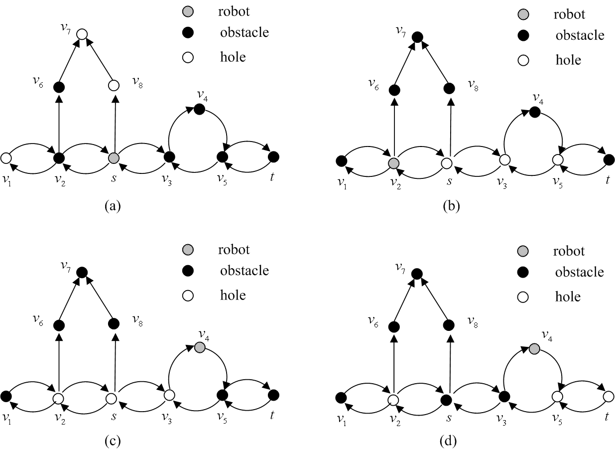
Figure 1: Motion planning on digraphs

Consider the strongly connected component $C$ in the graph of Figure 1 which contains vertices $v_{1},...,v_{5}$, $s$ and $t$. The initial positions of the robot and obstacles are shown in Figure 1(a).

We can move the robot from $s$ to $t$ as follows: move the hole in $v_{1}$ to $v_{2}$, move the robot from $s$ to $v_{2}$, then move the two holes in $v_{7}$, $v_{8}$ into $C$ through $s$, without moving the robot in $v_{2}$ (Figure 1(b)). Now move the obstacle in $v_{4}$ to $v_{5}$, and move the robot to $v_{4}$ (see Figure 1(c)). Move the two obstacles in $v_{5}$ and $t$ to $v_{3}$ and $s$ (Figure 1(d)), then move the robot from $v_{4}$ to $v_{5}$, and finally to $t$. The main idea of these moves is to move the robot to $v_{4}$ in order to free the way for the moves of the holes from $s$ and $v_{3}$ to $v_{5}$ and $t$.

If the robot is in $s$ and we move the hole in $v_{7}$ to $v_{2}$ (Figure 2(a)), then the problem becomes infeasible. We can move the robot from $s$ to $v_{2}$ and the hole in $v_{8}$ to $s$ (Figure 2(b)), but it is then impossible to move the robot from $v_{2}$ to $v_{4}$.

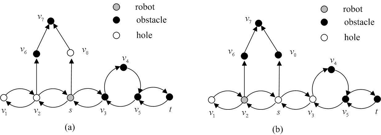
Figure 2: Object moves that do not preserve feasibility

As illustrated in the above example, the intricacy of motion planning on digraphs follows from the non-reversibility of moves in the digraphs.

In the sequel, we propose algorithms which take as input, a digraph $D=(V,E)$ encoded by its adjacency lists, a source and destination vertex $s,t\in V$, a function $f$ mapping each vertex to an element of the set {“robot”,“obstacle”, “hole”}, and produces a Boolean value (true or false) indicating whether it is feasible to move the robot from $s$ to $t$ in $D$.

3 Preliminaries

A digraph $D$ is a binary tuple $(V,E)$ such that $E\subseteq V^{2}$. Elements of $V$ and $E$ are called respectively vertices and arcs of $D$. We assume that $(v,v)\not\in E$ for all $v\in V$ (there are no self-loops).

For a vertex $v$ of a digraph $D=(V,E)$, the indegree of $v$, denoted $in(v)$, is defined as $\lvert\{w\in V|(w,v)\in E\}\rvert$, and the outdegree of $v$, denoted $out(v)$, is defined as $|\{w\in V|(v,w)\in E\}|$.

A graph $G$ is a binary tuple $(V,E)$ such that $E\subseteq V^{[2]}$, where $V^{[2]}$ contains exactly all two-element subsets of $V$, namely $V^{[2]}=\{\{v,w\}|v,w\in V,v\neq w\}$. Elements of $E$ are called edges of $G$.

For a vertex $v$ of a graph $G=(V,E)$, the degree of $v$, denoted $deg(v)$, is defined as $|\{w\in V|\{v,w\}\in E\}|$.

If $D=(V,E)$ (resp. $G=(V,E)$), and $e=(v,w)\in E$ (resp. $e=\{v,w\}\in E$), then $e$ is said to be incident to $v$ and $w$ in $D$ (resp. $G$).

A digraph (resp. graph) containing exactly one vertex is said to be trivial, otherwise it is said to be nontrivial.

Given a digraph $D=(V,E)$ (resp. graph $G=(V,E)$), the digraph (resp. graph) $H=(V_{H},E_{H})$ such that $V_{H}\subseteq V$ and $E_{H}\subseteq E$ is called a sub-digraph of $D$ (resp. subgraph of $G$). Let $X\subseteq V$, the sub-digraph (resp. subgraph) induced by $X$, denoted $D[X]$ (resp. $G[X]$), is the sub-digraph (resp. subgraph) $(X,E\cap X\times X)$ (resp. $(X,E\cap X^{[2]})$).

Suppose $D=(V,E)$ (resp. $G=(V,E)$) is a digraph (resp. graph) and $X\subseteq V$, let $D-X$ (resp. $G-X$) denote the digraph (resp. graph) obtained from $D$ (resp. $G$) by deleting all the vertices in $X$ and all the arcs (resp. edges) incident to at least one element of $X$. If $X=\{v\}$, then $D-\{v\}$ (resp. $G-\{v\}$) is written as $D-v$ (resp. $G-v$) for simplicity.

Given a digraph $D=(V,E)$, the underlying graph of $D$, denoted by $\mathcal{G}(D)$, is the graph obtained from $D$ by omitting the directions of arcs, namely $\mathcal{G}(D)=\left(V,\{\{v,w\}|(v,w)\in E\}\right)$.

A path of a digraph $D=(V,E)$ (resp. graph $G=(V,E)$) is an alternating sequence of vertices and arcs (resp. edges) $v_{0}e_{1}v_{1}...v_{k-1}e_{k}v_{k}$ ($k\geq 1$) such that for all $1\leq i\leq k$, $e_{i}=(v_{i-1},v_{i})\in E$ (resp. $e_{i}=\{v_{i-1},v_{i}\}\in E$), and for all $0\leq i<j\leq k$, $v_{i}\neq v_{j}$. $v_{0}$ and $v_{k}$ are called the tail and head endpoint of the path respectively, and the other vertices are called the internal vertices of the path. In particular, an arc or an edge is a path without internal vertices.

A cycle of a digraph $D=(V,E)$ is a sequence of vertices $v_{0}v_{1}...v_{k}$ such that for all $0\leq i\leq k$, $(v_{i},v_{i+1})\in E$ ($v_{k+1}$ interpreted as $v_{0}$), and for all $0\leq i<j\leq k$, $v_{i}\neq v_{j}$. Cycles of graphs can be defined similarly, but we have the additional restriction that $k\geq 2$. So cycles of graphs contain at least three vertices.

A digraph $D$ is acyclic if there are no cycles in $D$.

Suppose $H=(V_{H},E_{H})$ is a sub-digraph of $D=(V,E)$ (resp. subgraph of $G=(V,E)$). A path $P$ of $D$ (resp. $G$) is an $H$-path if the two endpoints of $P$ are in $H$, no internal vertices of $P$ are in $H$, and no arcs (resp. edges) of $P$ are in $H$. In particular, an arc $(v,w)\in E\backslash E_{H}$ (resp. an edge $\{v,w\}\in E\backslash E_{H}$) with $v,w\in V_{H}$ is an $H$-path. A cycle $C$ is an $H$-cycle if there is exactly one vertex of $C$ in $H$.

Let $H_{1}=(V_{1},E_{1})$ and $H_{2}=(V_{2},E_{2})$ be two sub-digraphs of a digraph $D=(V,E)$, then the union of $H_{1}$ and $H_{2}$, $H_{1}\cup H_{2}$, is defined as $\left(V_{1}\cup V_{2},E_{1}\cup E_{2}\right)$. The union of subgraphs can be defined similarly.

A digraph $D=(V,E)$ is strongly connected if for any two distinct vertices $v$ and $w$, there are both a path from $v$ to $w$ and a path from $w$ to $v$ in $D$. The digraph containing exactly one vertex and no arcs is the minimal strongly connected digraph.

Let $D=(V,E)$ be a digraph. The strongly connected components of $D$ are the maximal strongly connected sub-digraphs of $D$.

A graph $G=(V,E)$ is connected if for any two distinct vertices $v$ and $w$ of $G$, there is a path of $G$ with endpoint $v$ and $w$. The connected components of a graph $G$ are the maximal connected subgraphs of $G$.

If $G=(V,E)$ is a graph, $v\in V$, and the number of connected components of $G-v$ is more than that of $G$, then $v$ is said to be a cut vertex of $G$.

A graph $G$ is biconnected if $G$ is connected and there are no cut vertices in $G$. In particular, the graph containing exactly one vertex is the minimal biconnected graph. The biconnected components of a graph $G$ are the maximal biconnected subgraphs of $G$.

Without loss of generality, we assume that for each digraph $D$, (i) the underlying graph of $D$, $\mathcal{G}(D)$, is connected, (ii) the source vertex $s$ and the destination vertex $t$ are distinct (thus all the digraphs considered from now on are nontrivial), (iii) there is at least one path from $s$ to $t$ in $D$.

4 Motion planning on acyclic digraphs

In this section we assume that $D=(V,E)$ is an acyclic digraph.

We first recall a result about acyclic orderings of acyclic digraphs.

An acyclic ordering of an acyclic digraph $D=(V,E)$ is an ordering of all vertices of $D$, say $v_{1},\dots,v_{k}$, such that $(v_{i},v_{j})\in E$ implies $i<j$. From [BJG00], we know that an acyclic ordering of a given acyclic digraph can be computed in linear time by depth-first-search.

Theorem 1 ([BJG00]).

Given an acyclic digraph $D=(V,E)$, an acyclic ordering of $D$ can be computed in time $O(n+m)$, where $n$ is the number of vertices and $m$ is the number of arcs of $D$.

We introduce some notations in the following.

Let $V^{\prime}$ denote the set of vertices from which there is a path to $t$, and to which there is a path from $s$. In particular, $s,t\in V^{\prime}$.

For each $v\in V^{\prime}$, let $h(v)$ denote the number of holes that can be moved to $v$.

For each $v\in V^{\prime}$, define $h_{t}(v)$ as follows: Suppose that the robot is in $v$.

• If the robot can be moved from $v$ to $t$ in $D$, then there may be different paths (from $v$ to $t$) along which the robot can be moved from $v$ to $t$, let $h_{t}(v)$ be the minimal length (number of arcs) of such paths.

• If it is impossible to move the robot from $v$ to $t$, let $h_{t}(v)=\infty$.

The algorithm FAD($D,s,t,f$) (see Algorithm 1 in the box below) decides the feasibility of the motion planning problem on acyclic digraphs. FAD first computes $h(v)$ for each $v\in V^{\prime}$, then computes $h_{t}(v)$ for each $v\in V^{\prime}$, finally checks whether $h_{t}(s)<\infty$.

input : $(D,s,t,f)$ such that $D=(V,E)$ is an acyclic digraph, $s,t\in V$, $s\neq t$, and $f$ is a function from $V$ to {“robot”,“obstacle”,“hole”}.

output : true or false.

/* Compute $V^{\prime}$, the set of vertices reachable from $s$ and from which $t$ is reachable. */

Let $W$ be a FIFO queue, push $s$ into $W$.

foreach $v\in V$ do if $v=s$ then $srcReach(v):=true$. else $srcReach(v):=false$.

while $W$ is nonempty do  $w:=$the first element of $W$, pop the first element of $W$.

foreach $w^{\prime}$ such that $(w,w^{\prime})\in E$ do  if $srcReach(w^{\prime})=false$ then  $srcReach(w^{\prime}):=true$, push $w^{\prime}$ into $W$.       Push $t$ into $W$.

foreach $v\in V$ do if $v=t$ then $reachDest(v):=true$ else $reachDest(v):=false$

while $W$ is nonempty do  $w:=$the first element of $W$, pop the first element of $W$.

foreach $w^{\prime}$ such that $(w^{\prime},w)\in E$ do  if $reachDest(w^{\prime})=false$ then  $reachDest(w^{\prime}):=true$, push $w^{\prime}$ into $W$.       $V^{\prime}:=\{v\in V|srcReach(v)=reachDest(v)=true\}$.

/* Compute $h(v)$ */

foreach $v\in V^{\prime}$ do  foreach $v^{\prime}\in V$ do $idx(v^{\prime}):=false$

if $f(v)=$“hole” then $h(v):=1$. else $h(v):=0$.

Push $v$ into $W$.

while $W$ is nonempty do  $w:=$ the first element of $W$, pop the first element of $W$.

foreach $w^{\prime}\in V$ such that $(w,w^{\prime})\in E$ do  if $idx(w^{\prime})=false$ then  $idx(w^{\prime}):=true$, push $w^{\prime}$ into $W$.

if $f(w^{\prime})=$“hole” then $h(v):=h(v)+1$.         /* Compute $h_{t}(v)$ */

Compute an acyclic ordering of $D[V^{\prime}]$, say $v_{1},\dots,v_{k}$, such that $v_{1}=s,v_{k}=t$.

$h_{t}(v_{k}):=0$.

for $i$ from $k-1$ to $1$ do  if $\exists j:i<j\leq k$ such that $(v_{i},v_{j})\in E$ and $h(v_{j})\geq h_{t}(v_{j})+1$ then  $h_{t}(v_{i}):=\min\{h_{t}(v_{j})+1|(v_{i},v_{j})\in E,h(v_{j})\geq h_{t}(v_{j})+1\}$.

    if $h_{t}(s)<\infty$ then return true. else return false.

Algorithm 1 FAD($D,s,t,f$)

The computation of $h(v)$ and $h_{t}(v)$ on an acyclic digraph is illustrated in Figure 3.

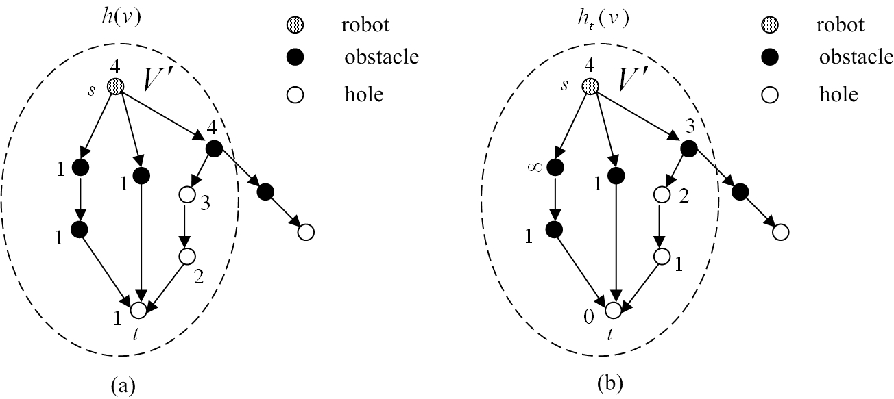
Figure 3: Computation of $h(v)$ and $h_{t}(v)$

Theorem 2.

FAD is correct.

Proof.

We prove that given an instance of the motion planning problem on acyclic digraphs, FAD returns true iff the problem is feasible.

“If” part:

If the problem is feasible, the robot can be moved from $s$ to $t$. Let $P$ be the trace of the robot during this movement (namely the sequence of nodes and arcs reached by the robot). As a result of acyclicity of $D$, $P$ is a path of $D$. Let $P=v_{0}e_{1}v_{1}\cdots v_{k-1}e_{k}v_{k}$ such that $v_{0}=s$ and $v_{k}=t$. During the movement, when the robot is moved to $v_{i-1}$($1\leq i\leq k$), in order to move the robot from $v_{i-1}$ to $v_{i}$, a hole should be moved to $v_{i}$. Since $D$ is acyclic, the hole moved to $v_{i}$ cannot be moved to $v_{j}$ for any $j$ such that $i<j\leq k$ (holes are moved along the reverse direction of arcs). So these holes are distinct from each other, and can be moved to occupy all the vertices on $P$ except $s$. By induction, we can show that for all vertices $v$ on $P$, $h_{t}(v)$ computed by FAD satisfies that $h_{t}(v)<\infty$. Consequently FAD returns true.

“Only if” part:

If FAD returns true, then $h_{t}(s)<\infty$. By induction, we can show that there is a path $P$ from $s$ to $t$ such that for each vertex $v\neq s$ on $P$, we have $h_{t}(v)<\infty$ and $h(v)\geq h_{t}(v)+1$, and for each arc $(v,w)$ on $P$, $h_{t}(v)=h_{t}(w)+1$. By induction again, we can show that the holes in $D$ can be moved to occupy all the vertices on $P$ except $s$. Then the robot can be moved to $t$ along $P$, the problem is feasible. ∎

Theorem 3.

The time complexity of FAD is $O(nm)$, where $n$ is the number of vertices, and $m$ is the number of arcs.

Proof.

Let $D$ be an acyclic digraph, $n$ and $m$ be the number of vertices and number of arcs of $D$ respectively.

The computation of $V^{\prime}$ takes $O(m)$ time since each arc is visited at most once in each of the first two “While” loops.

The computation of $h(v)$’s takes $O(nm)$ time because the computation of each $h(v)$ takes $O(m)$ time and there are at most $O(n)$ such computations.

The computation of an acyclic ordering of $D[V^{\prime}]$ takes $O(n+m)$ time from Theorem 1.

The computation of $h_{t}(v)$’s takes $O\left(\sum\limits_{v\in V^{\prime}}out(v)\right)=O(m)$ time.

Since $n\leq m$, we conclude that the time complexity of FAD is $O(m+nm+n+m+m)=O(nm)$. ∎

5 Structure of strongly connected digraphs

In this section, we consider the structure of strongly connected digraphs. We first recall some definitions and theorems.

An open ear decomposition of a digraph $D=(V,E)$ (resp. graph $G=(V,E)$) is a sequence of sub-digraphs of $D$ (resp. subgraphs of $G$), say $P_{0},...,P_{r}$, such that

• $P_{0}$ is a cycle;

• $P_{i+1}$ is a $D_{i}$-path (resp. $G_{i}$-path), where $D_{i}$ (resp. $G_{i}$) is $\bigcup\limits_{0\leq j\leq i}P_{j}$ for all $0\leq i<r$;

• $D=\bigcup\limits_{0\leq i\leq r}P_{i}$ (resp. $G=\bigcup\limits_{0\leq i\leq r}P_{i}$).

A closed ear decomposition of a digraph $D=(V,E)$ (resp. graph $G=(V,E)$) is a sequence of sub-digraphs of $D$ (resp. subgraphs of $G$), say $P_{0},...,P_{r}$, such that

• $P_{0}$ is a cycle;

• $P_{i+1}$ is a $D_{i}$-path or a $D_{i}$-cycle (resp. a $G_{i}$-path or a $G_{i}$-cycle), where $D_{i}$ (resp. $G_{i}$) is $\bigcup\limits_{0\leq j\leq i}P_{j}$ for all $0\leq i<r$;

• $D=\bigcup\limits_{0\leq i\leq r}P_{i}$ (resp. $G=\bigcup\limits_{0\leq i\leq r}P_{i}$).

Theorem 4 ([Wes00]).

Let $G$ be a graph containing at least three vertices. $G$ is biconnected iff $G$ has an open ear decomposition. Moreover, any cycle can be the starting point of an open ear decomposition.

Theorem 5 ([BJG00]).

Let $D$ be a nontrivial digraph. $D$ is strongly connected iff $D$ has a closed ear decomposition. Moreover, any cycle can be the starting point of a closed ear decomposition.

Let $G=(V,E)$ be a graph. The biconnected-component graph of $G$, denoted $\mathcal{G}_{bc}(G)$, is a bipartite graph $(V_{bc},W_{bc},E_{bc})$ defined by

• $V_{bc}$: biconnected components of $G$;

• $W_{bc}$: vertices of $G$ shared by at least two distinct biconnected components of $G$;

• $E_{bc}$: let $B\in V_{bc}$ and $w\in W_{bc}$, then $(B,w)\in E_{bc}$ iff $w\in V(B)$.

Theorem 6 ([Wes00]).

Let $G=(V,E)$ be a connected graph. Then $\mathcal{G}_{bc}(G)$ is a tree.

Now we introduce a new class of digraphs, strongly biconnected digraphs.

Definition 7.

Let $D$ be a digraph. $D$ is said to be strongly biconnected if $D$ is strongly connected and $\mathcal{G}(D)$ is biconnected. The strongly biconnected components of $D$ are the maximal strongly biconnected sub-digraphs of $D$.

In particular, the digraph containing exactly one vertex and no arcs is strongly biconnected.

We now show that strongly biconnected digraphs also admit a similar characterization.

Theorem 8.

Let $D$ be a nontrivial digraph. $D$ is strongly biconnected iff $D$ has an open ear decomposition. Moreover, any cycle can be the starting point of an open ear decomposition.

Proof.

“If” part: Suppose $D$ has an open ear decomposition $P_{0},\dots,P_{r}$.

Since open ear decompositions are special cases of closed ear decompositions, from Theorem 5, we know that $D$ is strongly connected.

Let $P^{\prime}_{i}=\mathcal{G}(P_{i})$, the underlying graph of $P_{i}$, for all $0\leq i\leq r$.

If $P_{0}$ is a cycle with at least $3$ vertices, then $P^{\prime}_{0},...,P^{\prime}_{r}$ is an open ear decomposition of $\mathcal{G}(D)$, $\mathcal{G}(D)$ is biconnected according to Theorem 4. So $D$ is strongly biconnected.

If $P_{0}$ is a cycle with only two vertices and $r=0$, then $\mathcal{G}(D)$ is a graph with exactly two vertices connected by an edge. $\mathcal{G}(D)$ is biconnected and $D$ is strongly biconnected.

Otherwise, $P_{0}$ is a cycle with only two vertices and $r>0$. Then it is easy to see that $P^{\prime}_{0}\cup P^{\prime}_{1}$ is a cycle of $\mathcal{G}(D)$, so $\left(P^{\prime}_{0}\cup P^{\prime}_{1}\right),P^{\prime}_{2},...,P^{\prime}_{r}$ is an open ear decomposition of $\mathcal{G}(D)$. $\mathcal{G}(D)$ is biconnected from Theorem 4. $D$ is strongly biconnected.

“Only if” part: Suppose $D$ is nontrivial and strongly biconnected. Consider the following procedure:

Initially select an arbitrary cycle in $D$, let $P_{0}$ be this cycle.

Suppose we have obtained $D_{i}=\bigcup\limits_{0\leq j\leq i}P_{j}$.

Select a $D_{i}$-path in $D$ as $P_{i+1}$.

Continue until $D_{i}=D$.

The above procedure produces the desired open ear decomposition of $D$, which is guaranteed by the following claim.

Claim. If $D_{i}\neq D$, there must be a $D_{i}$-path in $D$.

Proof of the Claim.

If $V(D)=V(D_{i})$, then there must be arcs in $D$ but not in $D_{i}$, which are the $D_{i}$-paths in $D$.

Otherwise, $V(D)\backslash V(D_{i})$ is nonempty.

To the contrary, suppose that there are no $D_{i}$-paths in $D$.

For all $v\in V(D)\backslash V(D_{i})$, we call the path from some vertex in $D_{i}$ to $v$ such that none of its internal vertices are in $D_{i}$, as the $(D_{i},v)$-path, and the path from $v$ to some vertex in $D_{i}$ such that none of its internal vertices are in $D_{i}$, as the $(v,D_{i})$-path. Moreover, we call the endpoint of a $(D_{i},v)$-path (resp.$(v,D_{i})$-path ) that is in $D_{i}$ as the $D_{i}$-endpoint of the $(D_{i},v)$-path (resp. $(v,D_{i})$-path).

Because $D$ is strongly connected, for all $v\in V(D)\backslash V(D_{i})$, there are $(D_{i},v)$-paths and $(v,D_{i})$-paths in $D$. Let $\textrm{End}(D_{i},v)$ and $\textrm{End}(v,D_{i})$ be the set of $D_{i}$-endpoints of $(D_{i},v)$-paths and $(v,D_{i})$-paths respectively.

For each $v\in V(D)\backslash V(D_{i})$, if $v^{\prime}\in\textrm{End}(D_{i},v)$ and $v^{\prime\prime}\in\textrm{End}(v,D_{i})$, then we must have $v^{\prime}=v^{\prime\prime}$, because otherwise we will have a $D_{i}$-path in $D$, contradicting to the assumption. Therefore for each $v\in V(D)\backslash V(D_{i})$, $\textrm{End}(D_{i},v)=\textrm{End}(v,D_{i})$, and $\textrm{End}(D_{i},v)$ is a singleton.

For all $v^{\prime}\in V(D_{i})$, let $F_{v^{\prime}}$ be the set of all $v\in V(D)\backslash V(D_{i})$ such that $\textrm{End}(D_{i},v)=\{v^{\prime}\}$.

Then all the nonempty $F_{v^{\prime}}$’s ($v^{\prime}\in V(D_{i})$) form a partition of $V(D)\backslash V(D_{i})$ (see Figure 4).

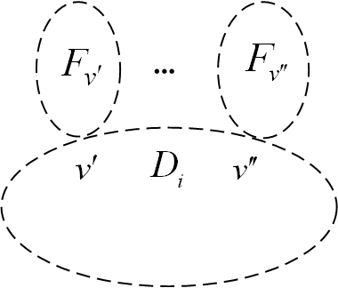
Figure 4: Partition of $V(D)\backslash V(D_{i})$

Select an arbitrary $v^{\prime}\in V(D_{i})$ such that $F_{v^{\prime}}$ is nonempty. We show that $v^{\prime}$ is a cut vertex in $\mathcal{G}(D)$.

Let $v$ be a vertex in $F_{v^{\prime}}$, we show that all the arcs incident to $v$ are confined to $F_{v^{\prime}}\cup\{v^{\prime}\}$, namely if $e=(v,w)\in E$ or $e=(w,v)\in E$, then $w\in F_{v^{\prime}}\cup\{v^{\prime}\}$.

To the contrary, suppose that there is an arc $e=(v,w)$ (the case of $e=(w,v)$ is similar) such that $w\not\in F_{v^{\prime}}\cup\{v^{\prime}\}$, then either $w\in V(D_{i})$ and $w\neq v^{\prime}$, or $w\in F_{v^{\prime\prime}}$ for some $v^{\prime\prime}\in V(D_{i})$ such that $v^{\prime\prime}\neq v^{\prime}$.

Since $\textrm{End}(D_{i},v)=\textrm{End}(v,D_{i})$ is a singleton, the former case is impossible.

For the latter case, we can get a $D_{i}$-path in $D$, contradicting to the assumption.

Therefore, all the arcs incident to $v$ are confined to $F_{v^{\prime}}\cup\{v^{\prime}\}$, as a consequence, all the paths in $\mathcal{G}(D)$ from $v$ to vertices in $\mathcal{G}(D_{i})$ go through $v^{\prime}$, $v^{\prime}$ is a cut vertex in $\mathcal{G}(D)$, contradicting to the fact that $\mathcal{G}(D)$ is biconnected (since $D$ is strongly biconnected).

Consequently, when $V(D)\backslash V(D_{i})$ is nonempty, there are always $D_{i}$-paths in $D$.

We conclude that the claim holds and complete the proof of the theorem.

∎

We can prove the following structural theorem for strongly connected digraphs.

Theorem 9.

Let $D=(V,E)$ be a strongly connected digraph. Then the strongly biconnected components of $D$ are those $D[V(B)]$, namely the sub-digraph of $D$ induced by $V(B)$, where $B$ is a biconnected component of $\mathcal{G}(D)$.

Proof.

Let $D=(V,E)$ be a strongly connected digraph.

If $D$ is trivial, then the result is obvious.

Otherwise, $D$ is nontrivial, let $B$ be a biconnected component of $\mathcal{G}(D)$.

It is sufficient to show that $D[V(B)]$ is strongly connected. If this holds, then $D[V(B)]$ is strongly biconnected. Because all the vertices of a strongly biconnected sub-digraph of $D$ are in some biconnected component of $\mathcal{G}(D)$ and $B$ is a biconnected component of $\mathcal{G}(D)$, $D[V(B)]$ is a maximal strongly biconnected sub-digraph of $D$, i.e. a strongly biconnected component of $D$. Since the union of all biconnected components of $\mathcal{G}(D)$ is $\mathcal{G}(D)$ itself, the theorem holds.

Now we show that $D[V(B)]$ is strongly connected.

Let $v,w\in V(B)$ such that $v\neq w$. Since $D$ is strongly connected, there must be a path $P$ from $v$ to $w$ in $D$. Now we show that $P$ is in $D[V(B)]$ as a matter of fact.

To the contrary, suppose that there is a vertex on $P$ not in $D[V(B)]$.

Let $v^{\prime}$ be the first vertex on $P$ (starting from $v$) not in $D[V(B)]$. Then there is $w^{\prime}\in V(B)$ on $P$ such that $(w^{\prime},v^{\prime})\in E$. Because $B$ is a biconnected component of $\mathcal{G}(D)$, and two distinct biconnected components contain at most one vertex in common according to Theorem 6, it follows that $v^{\prime}$ is in a biconnected component $B^{\prime}\neq B$ of $\mathcal{G}(D)$, and $w^{\prime}$ is the unique vertex shared by $B^{\prime}$ and $B$. Since $P$ is a path, we have that $w^{\prime}\neq w$, otherwise we have reached $w$ before $v^{\prime}$ on $P$, a contradiction. Because $w\in V(B)$ and $w\neq w^{\prime}$, we have that $w\in V(B)\backslash V(B^{\prime})$. Since $w^{\prime}$ is the unique vertex shared by $B$ and $B^{\prime}$, any path from $v^{\prime}$ to $w\in V(B)\backslash V(B^{\prime})$ has to visit $w^{\prime}$, so $P$ must visit $w^{\prime}$ again after visiting $v^{\prime}$, contradicting to the fact that $P$ is a path and there should be no vertices visited twice on a path.

Consequently for any $v,w\in V(B)$, $v\neq w$, there is a path in $D[V(B)]$ from $v$ to $w$, $D[V(B)]$ is strongly connected. ∎

From Theorem 9, we have the following definition for strongly-biconnected-component graph of a strongly connected digraph.

Definition 10.

Let $D$ be a strongly connected digraph, the strongly-biconnected-component graph of $D$, denoted $\mathcal{G}_{sbc}(D)=(V_{sbc},W_{sbc},E_{sbc})$, is $\mathcal{G}_{bc}\left(\mathcal{G}(D)\right)$, namely the biconnected-component graph of the underlying graph of $D$.

From the above definition and Theorem 6, we have the following corollary.

Corollary 11.

Let $D$ be a strongly connected digraph. Then $\mathcal{G}_{sbc}(D)$ is a tree.

Example 12 (Strongly-biconnected-component graph).

A strongly connected digraph $D$ (Figure 5(a)) and its strongly-biconnected-component graph $\mathcal{G}_{sbc}(D)$ (Figure 5(b)).

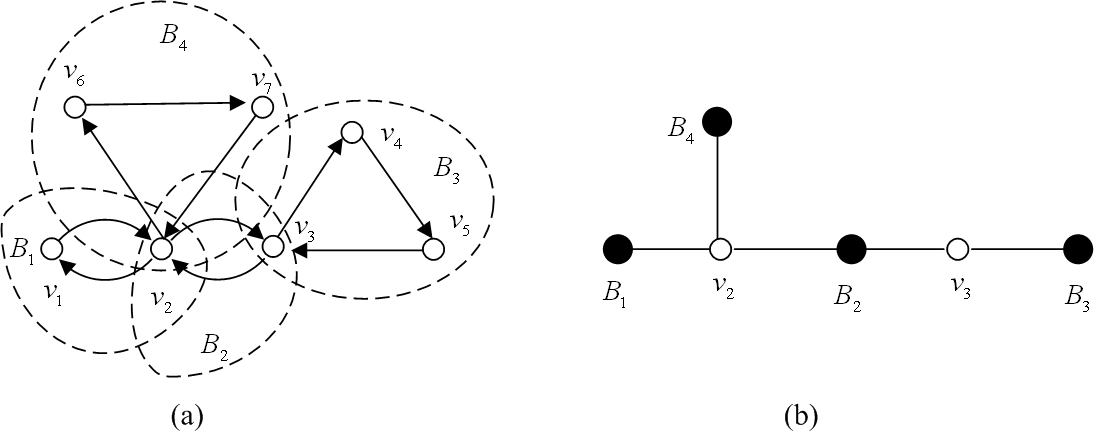
Figure 5: Example: strongly-biconnected-component graph

6 Motion planning on strongly connected digraphs

At first, we make the following observation about motion planning on strongly connected digraphs.

Proposition 13.

Let $D=(V,E)$ be a strongly connected digraph. Then

1. If the robot and a hole are in the same cycle $C$ of $D$, then the robot can be moved to any vertex of $C$.

2. The movement of objects (robot or obstacles) in $D$ preserves the feasibility of motion planning on $D$.

Proof.

(i): it is obvious since the hole can be moved along the reverse direction of the arcs in $C$ and the objects can be rotated to any vertex in $C$.

(ii): Suppose we move an object from $v$ to $w$ along the arc $(v,w)\in E$. We prove that the motion planning problem is feasible before the movement iff it is feasible after the movement.

Since $(v,w)\in E$ and $D$ is strongly connected, there is a path $P$ from $w$ to $v$ in $D$, let $C$ denote the cycle $P\cup\{(v,w)\}$.

Suppose the motion planning problem is feasible before the movement. Because after the movement, there is a hole in $v$, we can move the hole along the reverse direction of $C$, rotate the objects along $C$, and restore the situation before the movement, namely all the objects return to the positions before the movement. An example of this restoration is given in Figure 6. So the motion planning problem is also feasible after the movement.

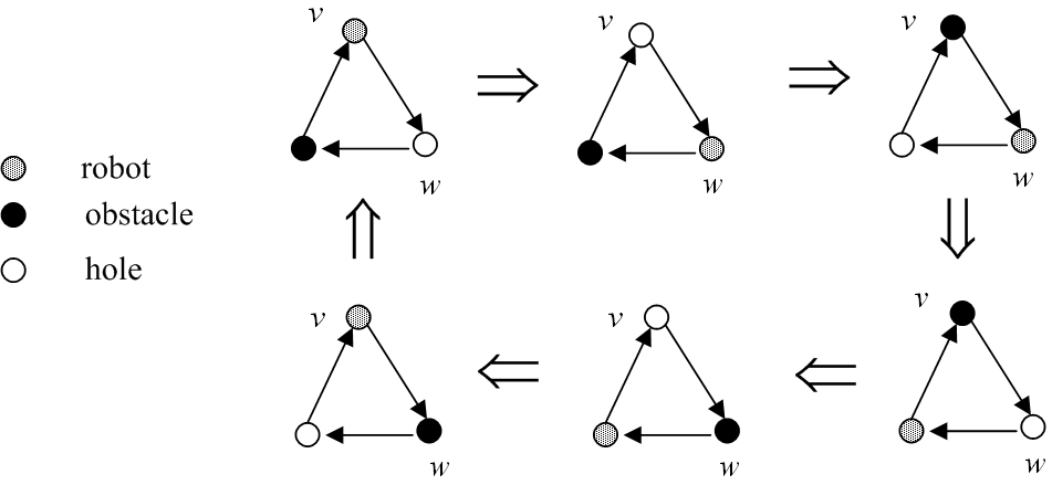
Figure 6: Restoration by rotating the objects in a cycle

The other direction is obvious. ∎

From [PRST94], we know that if a graph is biconnected, then one hole is sufficient to move the robot from the source vertex to the destination vertex, which is also the case for strongly biconnected digraphs.

Theorem 14.

Let $D$ be a strongly biconnected digraph. Then the motion planning problem on $D$ is feasible iff there is at least one hole in $D$.

Proof.

“Only if” part: obvious.

“If” part:

Suppose $D$ is strongly biconnected, there is exactly one hole in $D$ (the case that there are more than one hole is similar), the source vertex is $s$ and the destination vertex is $t$.

From Theorem 8, we know that there is an open ear decomposition $P_{0},...,P_{r}$ of $D$.

Let $j_{0}$ be the minimal $j$ such that $s,t$ and the hole are all in $D_{j}$, where $D_{j}=\bigcup\limits_{0\leq j^{\prime}\leq j}P_{j^{\prime}}$.

Induction on $j_{0}$.

Induction base $j_{0}=0$: $s$, $t$ and the hole are all in the cycle $P_{0}$. Then move the hole along the reverse direction of the cycle and move the robot to $t$.

Induction step $j_{0}>0$.

Let the tail and head endpoint of $P_{j_{0}}$ be $u^{\prime}$ and $v^{\prime}$ respectively.

Because of minimality of $j_{0}$, we have the following three cases.

Case I $s$ is in $P_{j_{0}}$, $s\neq u^{\prime},v^{\prime}$:

Select a path $P$ in $D_{j_{0}-1}$ from $v^{\prime}$ to $u^{\prime}$, then $P_{j_{0}}\cup P$ is a cycle in $D$.

If the hole is not in $P_{j_{0}}\cup P$, the hole must be in $D_{j_{0}-1}$, we can move it to $P$ in $D_{j_{0}}$ without moving the robot in $s$.

If $t$ is in $P_{j_{0}}\cup P$, then move the hole along the reverse direction of $P_{j_{0}}\cup P$ and move the robot to $t$.

Otherwise, move the hole along the reverse direction of $P_{j_{0}}\cup P$ and move the robot to $v^{\prime}$. Now the hole is in $P_{j_{0}}$, move the hole along the reverse direction of $P_{j_{0}}$, until it reaches $u^{\prime}$.

Then the position of the robot, $v^{\prime}$, the destination $t$ and the position of the hole, $u^{\prime}$, are all in $D_{j_{0}-1}$, according to the induction hypothesis, we can move the robot to $t$.

Case II $s$ is in $D_{j_{0}-1}$, the hole is in some vertex of $P_{j_{0}}$ different from $u^{\prime}$ and $v^{\prime}$:

Select a path $P$ in $D_{j_{0}-1}$ from $v^{\prime}$ to $u^{\prime}$, then $P_{j_{0}}\cup P$ is a cycle in $D$.

If $t$ is in $D_{j_{0}-1}$ and $s\neq u^{\prime}$, we can move the hole to $u^{\prime}$ along the reverse direction of $P_{j_{0}}$ without moving the robot in $s$, then according to the induction hypothesis, we can move the robot to $t$.

If $t$ is in $D_{j_{0}-1}$ and $s=u^{\prime}$, then move the hole along the reverse direction of $P_{j_{0}}\cup P$ and move the robot to $v^{\prime}$. Now the hole is in $P_{j_{0}}$, we can move the hole along the reverse direction of $P_{j_{0}}$ to $u^{\prime}$. Then by the induction hypothesis, we can move the robot to $t$.

If $t$ is not in $D_{j_{0}-1}$, then $t$ is in $P_{j_{0}}$.

If $s=u^{\prime}$, then we can move the hole along the reverse direction of $P_{j_{0}}\cup P$ and move the robot to $t$.

Now we consider the case $s\neq u^{\prime}$.

We can move the hole along the reverse direction of $P_{j_{0}}$ to $u^{\prime}$ without moving the robot. Then by the induction hypothesis, we can move the robot from $s$ to $v^{\prime}$ in $D_{j_{0}-1}$.

By the induction hypothesis again, we can move the robot from $v^{\prime}$ to $u^{\prime}$ in $D_{j_{0}-1}$. Let the trace of the robot during the movement from $v^{\prime}$ to $u^{\prime}$ be $P^{\prime}$. Note that $P^{\prime}$ may contain cycles. Suppose the last arc of $P^{\prime}$ is $(w,u^{\prime})$ for some $w$. Then the hole is in $w$ after the movement. Without loss of generality, we assume that during the movement, the robot visits $u^{\prime}$ only once since $u^{\prime}$ is the destination. Consequently, the hole can be moved from $w$ to $v^{\prime}$ along the reverse direction of $P^{\prime}$ without moving the robot in $u^{\prime}$ (see Figure 7).

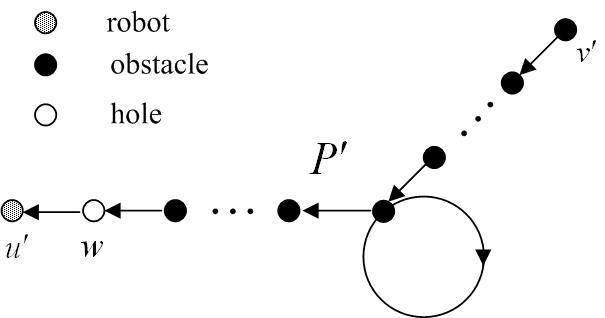
Figure 7: The case that the hole and $t$ are in $P_{j_{0}}$ different from $u^{\prime}$ and $v^{\prime}$, $s\in D_{j_{0}-1}$, and $s\neq u^{\prime}$

Since $P_{j_{0}}\cup P$ is a cycle, now we can move the hole along the reverse direction of $P_{j_{0}}\cup P$ and move the robot to $t$.

Case III $s$ and the hole are both in $D_{j_{0}-1}$, $t$ is in $P_{j_{0}}$, $t\neq u^{\prime},v^{\prime}$:

We can move the hole in $D_{j_{0}-1}$ to $v^{\prime}$ with possible movements of the robot in $D_{j_{0}-1}$. Suppose the new position of the robot is $s^{\prime}$.

Now move the hole to some vertex in $P_{j_{0}}$ different from $u^{\prime}$ and $v^{\prime}$, which is possible since $P_{j_{0}}$ contains at least three vertices. Then we have reduced Case III to Case II. ∎

We introduce the following notation before giving the algorithm.

Definition 15.

Let $D=(V,E)$ be a strongly connected digraph, $u,v,w\in V$ such that $v\neq w$, and $\mathcal{G}_{sbc}(D)=(V_{sbc},W_{sbc},E_{sbc})$ be the strongly-biconnected-component graph of $D$. Then $u$ is said to be on the $w$-side of $v$, if $u\neq v$ and one of the following two conditions holds:

1. $v\in W_{sbc}$, and $u,w$ are in the same connected component of $\mathcal{G}(D)-v$.

2. $v\not\in W_{sbc}$, and either $u,w$ are in the same connected component of $\mathcal{G}(D-V(B))$, or $u\in V(B)$, where $B$ is the unique strongly biconnected component of $D$ to which $v$ belongs.

$u$ is said to be on the non-$w$-side of $v$ if $u\neq v$, and $u$ is not on the $w$-side of $v$.

A hole (resp. obstacle) is said to be on the $t$-side of the robot if the position (vertex) of the hole (resp. obstacle) is on the $t$-side of the position of the robot, and a hole (resp. obstacle) is said to be on the non-$t$-side of the robot if the position of the hole is on the non-$t$-side of the position of the robot.

Note that if $u,v,w\in V$, $v\not\in W_{sbc}$, $v\neq w$, $v,w\in V(B)$, where $B$ is the unique strongly biconnected component of $D$ to which $v$ belongs, then $u$ is on the $w$-side of $v$ iff $u\neq v$ and $u\in V(B)$ according to Definition 15.

Example 16 ($t$-side of the robot).

In Figure 8(a), the robot is in $s\in W_{sbc}$, two holes in $v_{3}$ and $v_{4}$ are on the $t$-side of the robot, and the hole in $v_{1}$ is on the non-$t$-side of the robot. In Figure 8(b), the robot is in $v_{3}\not\in W_{sbc}$, the hole in $v_{2}$ belongs to the same strongly biconnected component as $v_{3}$, so $v_{2}$ is on the $t$-side of the robot, and two holes in $v_{1}$ and $s$ are on the non-$t$-side of the robot.

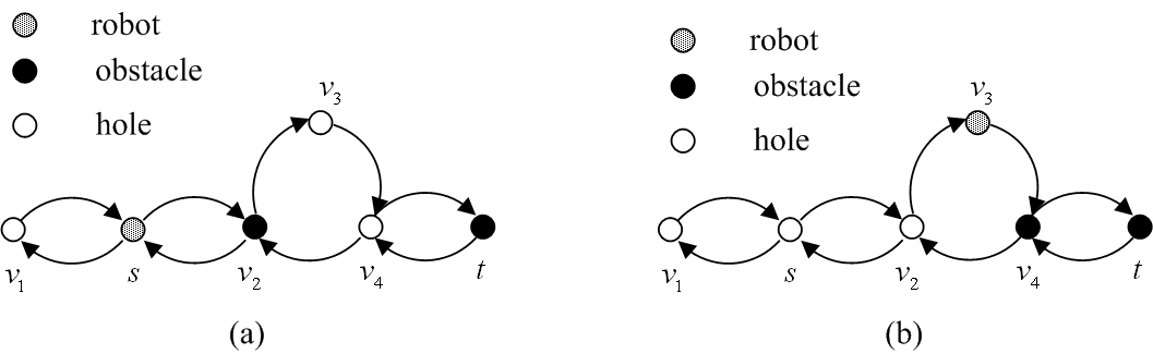
Figure 8: Example: $t$-side of the robot

Function FSCD (see Algorithm 2) decides the feasibility of motion planning problem on strongly connected digraphs. FSCD is similar to the algorithm for motion planning on graphs since strongly biconnected components of strongly connected digraphs are similar to biconnected components of connected graphs.

input : $(D,s,t,f)$ such that $D=(V,E)$ is a strongly connected digraph, $s,t\in V$, $s\neq t$, and $f$ is a function from $V$ to {“robot”,“obstacle”,“hole”}.

output : true or false.

Construct the underlying graph of $D$, $\mathcal{G}(D)$, and construct the biconnected-component graph of $\mathcal{G}(D)$ to get $\mathcal{G}_{sbc}(D)=(V_{sbc},W_{sbc},E_{sbc})$.

while there are obstacles on the $t$-side of the robot and there are holes on the non-$t$-side of the robot do  Let $v\in V$ be the current position of the robot.

if $v\in W_{sbc}$ then  Select a strongly biconnected component $B$ such that $v\in V(B)$, all the vertices of $B$ are not on the $t$-side of $v$, and there is at least one hole on the $w$-side of $v$ for some $w\in V(B)$, $w\neq v$.

if there are no holes in $B$ then  There is $w\in V(B)$ and $w\in W_{sbc}$ such that there is at least one hole on the non-$t$-side of $w$, move one such hole to $w$ without moving the robot.  

Move a hole in $B$ to $v$ and the robot is moved to some vertex $w^{\prime}\in V(B)$ such that $(v,w^{\prime})\in E$.

else  Let $B$ be the unique strongly biconnected component to which $v$ belongs ($B$ contains at least three vertices).

if there are no obstacles in $B$ then  Move an obstacle on the $t$-side of the robot into $B$ without moving the robot.   Move a hole on the non-$t$-side of the robot into $B$ by moving the robot if necessary, while keeping the robot inside $B$.

Move the robot to $v$ again.     Let the current position of the robot be $s^{\prime}$.

if $s^{\prime}$ and $t$ are in the same strongly biconnected component then  if there is at least one hole on the $t$-side of the robot then  return true. else  return false.  

else  Let $P=B_{0}v_{1}B_{1}...B_{r-1}v_{r}B_{r}$ be the path in $\mathcal{G}_{sbc}(D)=(V_{sbc},W_{sbc},E_{sbc})$, such that $s^{\prime}\in B_{0}$, $t\in B_{r}$, $s^{\prime}\neq v_{1}$ and $t\neq v_{r}$.

Let $l$ be the maximum of $j-i+1$ such that $1\leq i\leq j\leq r$, and $i,j$ satisfy the following conditions:

1. $i=1$, or $B_{i-1}$ contains at least three vertices, or there is some $B\in V_{sbc}$ such that $B$ is not on $P$ and $\{B,v_{i}\}\in E_{sbc}$;

2. $j=r$, or $B_{j}$ contains at least three vertices, or there is some $B\in V_{sbc}$ such that $B$ is not on $P$ and $\{B,v_{j}\}\in E_{sbc}$;

3. For all $i\leq k<j$, $B_{k}$ contains only two vertices, and for all $i<k<j$, there is no $B\in V_{sbc}$ such that $B$ is not on $P$ and $\{B,v_{k}\}\in E_{sbc}$.

if the number of holes on the $t$-side of the robot is no less than $l+1$ then  return true. else  return false.  

 

Algorithm 2 FSCD($D,s,t,f$)

Example 17 (Computation of FSCD).

The strongly connected digraph is given in Figure 9(a). At first, the robot is moved from $s$ to $v_{1}$, all the holes are on the $t$-side of the robot (see Figure 9(b)). Then according to the definition of $l$ in FSCD, we have $l=3$. There are four holes on the $t$-side of the robot, so FSCD returns “true”. Now we show how the robot is moved from $v_{1}$ to $t$ with the four holes: three holes are moved to $s,v_{2},v_{8}$ and the robot is moved to $v_{8}$ (see Figure 9(c)), then the holes are moved to $v_{2},v_{3},v_{4},v_{9}$ (See Figure 9(d)), the robot is moved to $v_{9}$ (see Figure 9(e)), and all the holes are moved to $v_{5},v_{6},v_{7},t$ (see Figure 9(f)), finally the robot is moved to $t$.

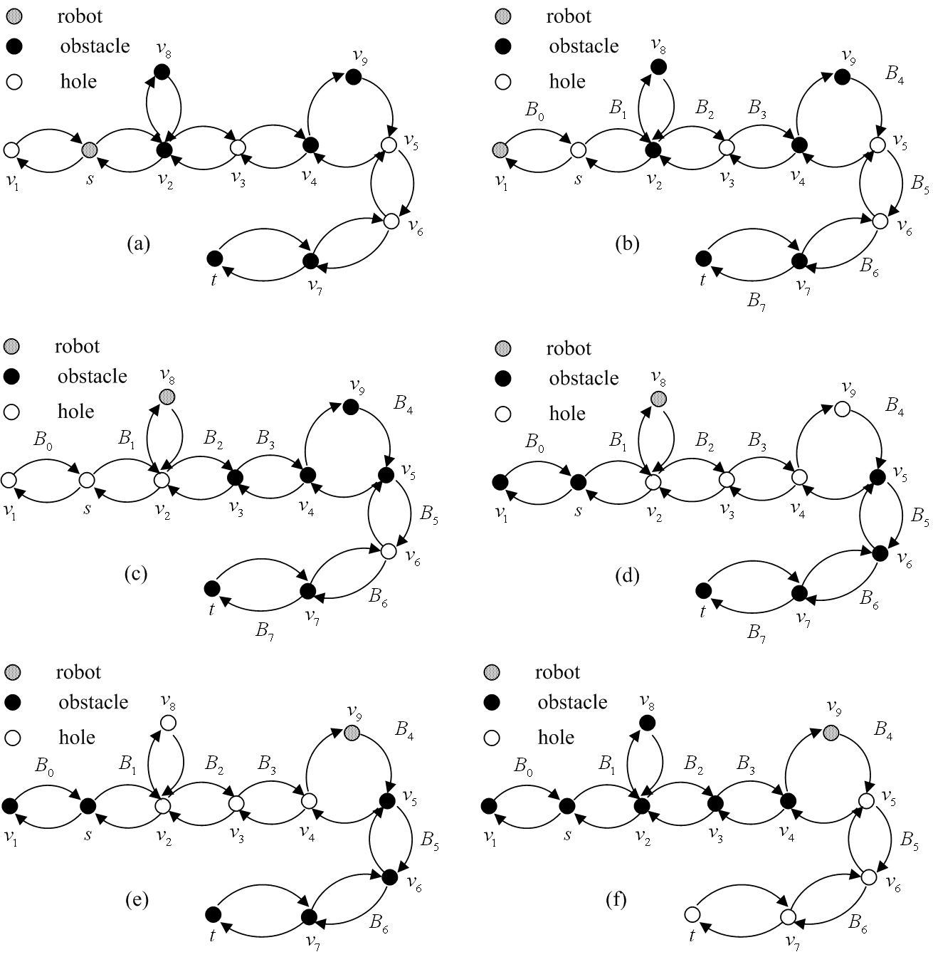
Figure 9: Example: motion planning on a strongly connected digraph

Theorem 18.

FSCD is correct.

Proof.

At first, we show that the “While” loop in FSCD terminates.

It is sufficient to show that each execution of the body of the “While” loop reduces the number of holes on the non-$t$-side of the robot by $1$.

There are two cases.

Case the robot is in some $v\in W_{sbc}$.

Then $v$ is shared by several strongly biconnected components.

Because there are holes on the non-$t$-side of the robot, we can select a strongly biconnected component $B$ such that $v\in V(B)$, all the other vertices of $B$ different from $v$ are on the non-$t$-side of $v$, and there is at least one hole on the $w$-side of $v$ for some $w\in V(B)$, $w\neq v$.

If there are no holes in $B$, then there is $w^{\prime}\in V(B)$ and $w^{\prime}\in W_{sbc}$ such that there is at least one hole on the non-$t$-side of $w^{\prime}$, then one such hole can be moved to $w^{\prime}$ without moving the robot.

Now there must be at least one hole in some $w^{\prime}\in V(B)$, there is a path from $v$ to $w^{\prime}$ in $B$, we can move the hole from $w^{\prime}$ to $v$ along the reverse direction of the path, and the robot is moved to $w^{\prime\prime}$ on the path such that $(v,w^{\prime\prime})\in E$.

The hole moved to $v$ is on the non-$t$-side of the robot before the movement. Now we show that the hole (in $v$) is on the $t$-side of the robot after the movement according to Definition 15: if $w^{\prime\prime}\in W_{sbc}$, then $v$ is in the same connected component as $t$ in $\mathcal{G}(D)-w^{\prime\prime}$, the hole in $v$ is on the $t$-side of the robot ($w^{\prime\prime}$); if $w^{\prime\prime}\not\in W_{sbc}$, since $B$ is the unique strongly biconnected component to which $w^{\prime\prime}$ belongs, and $v$ is in $B$, so the hole in $v$ is on the $t$-side of the robot ($w^{\prime}$) as well.

Consequently, in the case that the robot is in some $v\in W_{sbc}$, each execution of the “While”-loop reduces the number of holes on the non-$t$-side of the robot by $1$.

Case the robot is in some $v\not\in W_{sbc}$.

Let $B$ be the unique strongly biconnected component to which $v$ belongs.

Since there are holes on the non-$t$-side of the robot, and according to Definition 15, holes in $B$ are on the $t$-side of the robot, there must be some $w\in V(B)$, $w\neq v$, $w\in W_{sbc}$ such that there is at least one hole on the non-$t$-side of $w$.

Because there are obstacles on the $t$-side of the robot, if there are no obstacles in $B$, we can move an obstacle on the $t$-side of $v$ into $B$ without moving the robot. Now there must be at least one obstacle in $B$.

If $w$ is not occupied by an obstacle, then an obstacle in $B$ can be moved to $w$ by moving the robot if necessary. Now a hole on the non-$t$-side of $w$ can be moved to $w$. Move the robot to $v$ again.

In this case, one hole on the non-$t$-side of the robot is moved into $B$ and the robot returns to $v$ after the movement. Consequently, in this case, the number of holes on the non-$t$-side of the robot is reduced by $1$ as well.

After the execution of the “While” loop, either there are no obstacles on the $t$-side of the robot or all the holes are on the $t$-side of the robot. In the former case, it is evident that FSCD returns “true” eventually. Now we consider the latter case.

Suppose the current position of the robot is $s^{\prime}$ now.

If $s^{\prime}$ and $t$ are in the same strongly biconnected component $B$, then it is easy to see that the problem is feasible iff there is at least one hole on the $t$-side of the robot according to Theorem 14.

Otherwise, let $l$ be the number as defined in FSCD, we show that the problem is feasible iff there are at least $l+1$ holes.

“Only If” part: Suppose the problem is feasible.

Then according to Proposition 13, it is still feasible after the execution of the “While”-loop.

To the contrary, suppose that there are at most $l$ holes.

Let $P=B_{0}v_{1}B_{1}...B_{r-1}v_{r}B_{r}$ be the path in $\mathcal{G}_{sbc}(D)=(V_{sbc},W_{sbc},E_{sbc})$, such that $s^{\prime}\in B_{0}$, $t\in B_{r}$, $s^{\prime}\neq v_{1}$ and $t\neq v_{r}$.

Let $i,j:1\leq i,j\leq r$ satisfy Condition 1-3 in FSCD and $l=j-i+1$.

Since the problem is feasible, during the movement of the robot from $s^{\prime}$ to $t$, the robot should be moved to $v_{i}$ sometime.

If the robot has been moved to $v_{i}$, then there must be one hole on the non-$t$-side of $v_{i}$. So there are at most $l-1$ holes on the $t$-side of $v_{i}$. Since $l-1$ holes are needed to occupy all the vertices $v_{i+1},\cdots,v_{j}$ and move the robot from $v_{i}$ to $v_{j}$, if the robot has been moved from $v_{i}$ to $v_{j}$, then all the holes are on the non-$t$-side of $v_{j}$ now. The robot cannot be moved further towards $t$, namely the robot cannot be moved to the vertices on the $t$-side of $v_{j}$, the problem is infeasible, a contradiction.

“If” part: Suppose there are at least $l+1$ holes on the $t$ side of the robot.

Now we show how to move the robot from $s^{\prime}$ to $t$.

Let $i_{1}\cdots i_{p}$ ($i_{1}<i_{2}<...<i_{p}$) be the list of all the numbers $i_{j}$ such that $1\leq i_{j}<r$, and one of the following two conditions holds,

• $B_{i_{j}}$ contains at least three vertices,

• there is some $B\in V_{sbc}$ not on $P$ satisfying that $\{B,v_{i_{j}}\}\in E_{sbc}$.

Without loss of generality, assume that there is at least one $i_{j}$ satisfying the above condition. The case that there are no such $i_{j}$’s can be discussed similarly.

By convention, let $i_{0}=0$.

At first, we show how to move the robot from $B_{i_{0}}$ to $B_{i_{1}}$ if $i_{1}$ satisfies the first condition, and how to move the robot from $B_{i_{0}}$ to some $v$ in $B$ such that $B$ is not on $P$, $\{B,v_{i_{1}}\}\in E_{sbc}$, and $(v_{i_{1}},v)\in E$, if $i_{1}$ satisfies the second condition.

If $B_{i_{1}}$ contains at least three vertices, since $l\geq i_{1}$ and all the holes are on the $t$-side of the robot, we can move the holes to occupy all the $v_{j}$’s such that $1\leq j\leq i_{1}$ and let another hole occupy some vertex in $B_{i_{1}}$ different from $v_{i_{1}}$. Then we move the robot to $v_{1}$ (which is possible according to Theorem 14). We continue moving the robot to $v_{2}$, $\cdots$, until to $v_{i_{1}}$. Moreover, because there is still one hole in $B_{i_{1}}$, we can move the robot inside $B_{i_{1}}$ and move one hole to $v_{i_{1}+1}$ and all the other holes to the $t$-side of the $v_{i_{1}+1}$.

If there is some $B$ not on $P$ such that $\{B,v_{i_{1}}\}\in E_{sbc}$, since $l\geq i_{1}$, we let the holes occupy all the $v_{j}$’s such that $1\leq j\leq i_{1}$ and another hole occupy some $v\in V(B)$ such that $(v_{i_{1}},v)\in E$. Then we move the robot to $v_{i_{1}}$, and to $v$. Now we can move one hole to $v_{i_{1}}$ and all the other holes to the $t$-side of $v_{i_{1}}$.

The discussions for $i_{j}$ and $i_{j+1}$ ($2\leq j<p$) are similar to the above discussion.

During the movement, if sometime there are no obstacles on the $t$-side of the robot, then obviously the robot can be moved to $t$ and the problem is feasible. In the following we consider situations that such situation does not occur.

Now we assume that

1. If $B_{i_{p}}$ contains at least three vertices, then the robot is in $B_{i_{p}}$, one hole is in $v_{i_{p}+1}$, and all the other holes are on the $t$-side of $v_{i_{p}+1}$.

2. If there is $B\in V_{sbc}$ not on $P$ such that $\{B,v_{i_{p}}\}\in E_{sbc}$, then the robot is in some $v\in V(B)$ such that $\left(v_{i_{p}},v\right)\in E$, one hole is in $v_{i_{p}}$, and all the other holes are on the $t$-side of $v_{i_{p}}$.

In the first case above, since $l\geq r-i_{p}$, we can move one hole to some $w\in V(B_{r})$ such that $w\neq v_{r}$, and the other holes to occupy vertices $v_{i_{p}+1},\cdots,v_{r}$. Then we can move the robot to $v_{i_{p}+1}$, $\cdots$, until to $v_{r}$. Finally move the robot to $t$ inside $B_{r}$.

In the second case above, since $l\geq r-{i_{p}}+1$, we can move one hole to some $w\in V(B_{r})$ such that $w\neq v_{r}$, and the other holes to occupy $v_{i_{p}},\cdots,v_{r}$. Then we can move the robot to $v_{i_{p}}$, $\cdots$, until to $v_{r}$. Finally move the robot to $t$ inside $B_{r}$.

∎

Theorem 19.

The time complexity of FSCD is $O(nm)$, where $n$ is the number of vertices and $m$ is the number of arcs.

Proof.

There are three phases in FSCD: the phase constructing $\mathcal{G}_{sbc}(D)$, the phase of the “While”-loop, and the phase checking whether the number of holes are sufficient to move the robot to the destination.

The phase constructing $\mathcal{G}_{sbc}(D)$ is in time $O(m)$ since the biconnected components of a connected graph of $m$ edges can be constructed in $O(m)$ time by a depth-first-search technique [CLRS01].

Each execution of the “While”-loop takes $O(m)$ time, and there are at most $n$ such executions since there are at most $n$ holes, so the “While” loop takes $O(nm)$ time in total.

The phase checking whether the number of holes are sufficient to move the robot to the destination takes $O(m)$ time as well.

So the total time of FSCD is $O(nm)$. ∎

7 Conclusion

In this paper, we considered the feasibility of motion planning on digraphs, and proposed two algorithms to decide the feasibility of motion planning on acyclic and strongly connected digraphs respectively, we proved the correctness of the two algorithms and analyzed their time complexity. We showed that the feasibility of motion planning on acyclic and strongly connected digraphs can be decided in time linear in the product of the number of vertices and the number of arcs.

The algorithm for the feasibility of motion planning on acyclic digraphs (FAD) can be adapted to the case where the capacity of each vertex is more than one (namely, vertices are able to hold several objects simultaneously), by just changing the computation of the $h(v)$’s, the number of holes that could be moved to each node $v$. The algorithm for the feasibility of motion planning on strongly connected digraphs (FSCD) can also be adapted to the case where the capacity of each vertex is more than one by only changing the “While”-loop.

The strongly biconnected digraphs introduced in this paper may be of independent interest in graph theory since they admit nice characterization: a nontrivial digraph is strongly biconnected iff it has an open ear decomposition. It seems interesting to consider also strongly triconnected digraphs, strongly four-connected digraphs, etc. and investigate their theoretical properties.

The feasibility of motion planning on digraphs is only partially solved in this paper since we did not give the algorithm for deciding the feasibility on general digraphs, which, as well as the optimization of the motion of robot and obstacles, is much more intricate than that on graphs because of the irreversibility of the movements on digraphs.

The motion planning on graphs with one robot, GMP1R, has a natural generalization, GMP$k$R, where there are $k$ robots with their respective destinations. It is also interesting to consider motion planning on digraphs with $k$ robots since in practice it is more reasonable that a robot shares its workspace with other robots.

GMP$k$R in general is a very complex problem. A special case of GMP$k$R, where there are no additional obstacles (thus all the movable objects have their destinations), has been considered. Wilson studied the special case of GMP$k$R for $k=n-1$ in [Wil74], which is a generalization of the “15-puzzle” problem to general graphs. They gave an efficiently checkable characterization of the solvable instances of the problem. Kornhauser et al. extended this result to $k\leq n-1$ [KMS84]. Goldreich proved that determining the shortest move sequence for the problem studied by Kornhauser et al. is NP-hard [Gol84]. It seems more realistic to first consider the above special case of GMP$k$R on digraphs.

References

- [AMPP96] V. Auletta, A. Monti, D. Parente, and G. Persiano, A linear time algorithm for the feasibility of pebble motion on trees, SWAT ’96: Proceedings of the 5th Scandinavian Workshop on Algorithm Theory, LNCS 1097, Springer-Verlag, 1996, pp. 259–270.
- [AP01] V. Auletta and P. Persiano, Optimal pebble motion on a tree, Informaiton and Computation 165 (2001), no. 1, 42–68.
- [BJG00] J. Bang-Jensen and G. Gutin, Digraphs: Theory, algorithms and applications, springer monographs in mathematics, Springer-Verlag, 2000.
- [CLRS01] Thomas H. Cormen, Charles E. Leiserson, Ronald L. Rivest, and Clifford Stein, Introduction to algorithms, second edition, The MIT Press, 2001.
- [FK99] P. W. Finn and L. E. Kavmkit, Computational approaches to drug design, Algorithmica 25 (1999), 347–371.
- [Gol84] O. Goldreich, Finding the shortest move-sequence in the graph-generalized 15-puzzle is NP-hard, manuscript, 1984.
- [JJ06] Jorjeta G. Jetcheva and David B. Johnson, Routing characteristics of ad hoc networks with unidirectional links, Ad Hoc Networks 4 (2006), no. 3, 303–325.
- [KMS84] D. Kornhauser, G. Miller, and P. Spirakis, Coordinating pebble motion on graphs, the diameter of permutation groups, and applications, FOCS’84, 1984, pp. 241–250.
- [Lat95] Jean-Claude Latombe, Controllability, recognizability, and complexity issues in robot motion planning, FOCS, 1995, pp. 484–500.
- [LaV06] Steven M. LaValle, Planning algorithms, Cambridge University Press, 2006.
- [MD02] Mahesh K. Marina and Samir R. Das, Routing performance in the presence of unidirectional links in multihop wireless networks, in Proc. of ACM MobiHoc, 2002, pp. 12–23.
- [MPG] Motion planning game, website, http://www.download-game.com/Motion_Planning_Game.htm.
- [Per88] Yvonne Perrott, Track transportation systems, European patent, 1988, http://www.freepatentsonline.com/EP0284316.html.
- [PRST94] C. H. Papadimitriou, P. Raghavan, M. Sudan, and H. Tamaki, Motion planning on a graph, FOCS’94, 1994, pp. 511–520.
- [SA01] Guang Song and Nancy M. Amato, Using motion planning to study protein folding pathways, RECOMB ’01: Proceedings of the fifth annual international conference on Computational biology (New York, NY, USA), ACM, 2001, pp. 287–296.
- [Wes00] Douglas B. West, Introduction to graph theory, second edition, Prentice Hall, 2000.
- [Wil74] R. M. Wilson, Graph puzzles, homotopy, and the alternating group, Journal of Combinatorial Theory (B) 16 (1974), 86–96.